Model fitting and inference under Latent Equilibrium Processes

Abstract

This paper presents a methodology for model fitting and inference in the context of Bayesian models of the type f(Y | X, θ)f(X | θ)f(θ), where Y is the (set of) observed data, θ is a set of model parameters and X is an unobserved (latent) stationary stochastic process induced by the first order transition model f(X^(t+1) | X^(t), θ), where X^(t) denotes the state of the process at time (or generation) t. The crucial feature of the above type of model is that, given θ, the transition model f(X^(t+1) | X^(t), θ) is known but the distribution of the stochastic process in equilibrium, that is f(X | θ), is, except in very special cases, intractable, hence unknown. A further point to note is that the data Y has been assumed to be observed when the underlying process is in equilibrium. In other words, the data is not collected dynamically over time.

We refer to such specification as a latent equilibrium process (LEP) model. It is motivated by problems in population genetics (though other applications are discussed), where it is of interest to learn about parameters such as mutation and migration rates and population sizes, given a sample of allele frequencies at one or more loci. In such problems it is natural to assume that the distribution of the observed allele frequencies depends on the true (unobserved) population allele frequencies, whereas the distribution of the true allele frequencies is only indirectly specified through a transition model.

As a hierarchical specification, it is natural to fit the LEP within a Bayesian framework. Fitting such models is usually done via Markov chain Monte Carlo (MCMC). However, we demonstrate that, in the case of LEP models, implementation of MCMC is far from straightforward. The main contribution of this paper is to provide a methodology to implement MCMC for LEP models. We demonstrate our approach in population genetics problems with both simulated and real data sets. The resultant model fitting is computationally intensive and thus, we also discuss parallel implementation of the procedure in special cases.

1 Introduction

In this paper we present a class of hierarchical Bayesian models whose fitting has not received attention in the literature. We propose to work in the general structure that dates at least to Berliner (1996), Wikle et al. (1998) and more recently advocated in Clark et al. (2005); it can be described as f(data|process,parameters) × f(process|parameters) × f(parameters). More precisely, we are interested in settings where the process is assumed to be in equilibrium at the time of data collection but we do not know the form of the joint distribution of the process components or variables at equilibrium. In particular, we will assume that equilibrium is defined dynamically as the result of transitions arising under f(process state at time t+1|process state at time t, parameters) where t indexes, e.g., time period or generation. (The process need not be restricted to first order.) The process state space may be continuous or discrete and, typically, is high dimensional. However, we do insist upon there being a unique stationary or equilibrium distribution associated with the specified transition kernel (distribution). Usually the existence of such a unique distribution is straightforward to establish (see, e.g., Nummelin (1984), Meyn and Tweedie (1993)) but the explicit form is not available. For fitting these models standard MCMC methods are inapplicable. Our main contribution is to provide a computationally intensive alternative strategy.

Such models are natural in population genetics where an objective is to model allele frequencies at the population level. Data is usually collected from the population model in the form of allele frequencies at a set of loci for a collection of populations. The process model is described, for the ith population, in terms of say N_i, the number of diploid individuals in the ith population along with a vector of allele frequencies, p_il at locus l for that population. Specification of the mutation and migration structure provides the stochastic model for generation to generation transition in population frequencies. Inference is sought regarding the population sizes and the mutation and migration rates. The random vectors of allele frequencies over the populations and loci comprise the state of the process at any generation and are of less interest. Two other examples we describe below are in community biodiversity and metapopulation dynamics.

Another promising setting for the use of our methodology is in the development of forward simulation models. Here, we offer the opportunity to tune forward simulators in the model fitting process. This seems preferable to having to run them repeatedly at fixed parameter values in an attempt to ascertain values to align, in some fashion, the output with observed data. Such simulators are routinely used to model latent ecological processes (see, e.g., Turchin (2003); Shugart (2004), to provide output from global and regional climate models and to develop pollution surfaces (Kalnay (2003)). Further potential settings include economic equilibrium models, complex queueing and renewal processes, population diffusion process specified through (stochastic) differential equations but implemented through finite difference models, and perhaps even particle equilibrium models associated with electrical or magnetic fields.

To fix ideas, we assume that the posterior corresponding to the Bayesian model takes the form

$$f(\theta ,\mathbf{X}\mid \mathbf{Y})\propto f(\mathbf{Y}\mid \mathbf{X},\theta )f(\mathbf{X}\mid \theta )f\left(\theta \right)$$ (1)

In (1), Y is the observed data, X is an unobserved (latent) stationary stochastic process and θ is the set of model parameters. When the functional forms of each of the factors in (1) are known, fitting the model using MCMC is conceptually straightforward (though, of course, it can be challenging). However, we focus on the case where the functional form of f(X | θ) is unknown but is induced by a known transition model f(X^(t+1) | X^(t), θ), where X^(t) denotes the state of the stochastic process at time (or generation) t.

A key point is that our approach is an alternative to the more customary strategy of attempting a direct model of the process in equilibrium. We take advantage of the mechanistic knowledge of the evolution of the process and works with directly interpretable parameters. The resultant distributional specification for f(Y | X) is precisely the model we would use if we could write it down. In Section 3 we provide an example that demonstrates our assertion.

Another important point is the distinction between the above modelling scenario and that for dynamic models. In the latter situation, data is collected dynamically while in our setting, data is collected only when the underlying latent process is in equilibrium. Hence, methods like sequential Monte Carlo (for complete details, see Doucet et al. (2001) and Liu (2001)), appropriate for fitting dynamic models, are inappropriate in our situation. The key idea is the estimation of f(X | θ) using the available transition model.

The paper is structured as follows. The model fitting methodology for LEP models is developed in Section 2. Specialization of the proposed methodology to a problem of population genetics is discussed in Section 3. Section 4 presents simulation based applications of our methodology to the problem discussed in Section 3. Development of an algorithm for parallel implementation of our methodology to a generalized version of the population genetics problem and relevant simulation studies for the problem are presented in Section 5. Application of the methodology to a real data set is discussed in Section 6. In Section 7 we briefly develop the community biodiversity and metapopulation dynamics examples. Finally, we offer some concluding discussion in Section 8.

2 Proposed MCMC strategy for updating the parameters

2.1 Approximation of the functional form of f(X | θ)

The form of the Bayesian model is

$$f(\mathbf{Y}\mid \mathbf{X},\theta )f(\mathbf{X}\mid \theta )f\left(\theta \right)$$ (2)

MCMC is customarily used to iteratively update draws of (X, θ) to obtain samples from the posterior associated with (2). Computation of the acceptance ratio involves evaluation of (2) at the new and the current values of the parameters, the new value proposed from some arbitrary distribution. But since in (2), f(X | θ) is analytically intractable the acceptance ratio can not be evaluated. However, we can obtain an approximation to f(· | θ) directly through the transition kernel f(X^t+1 | X^(t), θ) as follows

$$\begin{array}{cc}\hfill f(\mathbf{X}\mid \theta )& =\int f(\mathbf{X}\mid \mathbf{Z},\theta )f(\mathbf{Z}\mid \theta )d\mathbf{Z}\hfill \\ \hfill & \approx \frac{1}{B}\underset{b=1}{\overset{B}{\Sigma }}f(\mathbf{X}\mid {\mathbf{Z}}^{\left(b\right)},\theta )\hfill \\ \hfill & \equiv {\tilde{f}}_B(\mathbf{X}\mid \theta )\hfill \end{array}$$ (3)

In (3), Z^(b); b = 1, … , B, are samples drawn from f(· | θ), obtained by running a sufficiently long trajectory of the transition model for a given θ. Since the f(X | Z^(b), θ) are known, f̃_B(X | θ) is analytically tractable. We propose to replace f(X | θ) with f̃_B(X | θ) in implementing the MCMC updates. It is important to note that, though we suppress it notationally, the set of Z^(b) depend upon θ; there will be a different set for each θ. Indeed, to ensure that f̃_B is well-defined, we need to guarantee that each time we select a particular value of θ, we obtain the same set of Z's. Computationally, this is most easily accomplished by fixing the seed in the random number generator that is employed. Furthermore, since θ will be updated at each iteration, the computationally intensive nature of our approach begins to emerge.

2.2 Updating parameters

Recall the general form of the acceptance ration for an MCMC algorithm to sample say g(U) using an importance sampling density h(U), i.e., $\min (1,\frac{g\left({\mathbf{U}}^{\mathit{new}}\right)h\left({\mathbf{U}}^{\mathit{curr}}\right)}{g\left({\mathbf{U}}^{\mathit{curr}}\right)h\left({\mathbf{U}}^{\mathit{new}}\right)})$ for current (curr) and new (new) values. Hence, if we propose to update (X, θ) in (2) we obtain the simple acceptance ratio, $\min (1,\frac{f(\mathbf{Y}\mid {\mathbf{X}}^{\mathit{new}},{\theta }^{\mathit{new}})}{f(\mathbf{Y}\mid {\mathbf{X}}^{\mathit{curr}},{\theta }^{\mathit{curr}})})$. Unfortunately the dimension of X and θ will jointly be much too large for a single block update; the chain will never move. So, we have to consider sub-block, perhaps even component-level updating.

We make a clarification of (2) to

$$f(\mathbf{Y}\mid \mathbf{X},\alpha )f(\mathbf{X}\mid \theta )f\left(\alpha \right)f\left(\theta \right)$$ (4)

In (4), we have separated the process parameters from those that are associated with the data model. Updating α is familiar and does not warrant further discussion; it may be done as a block or component-wise according to the specifications. As for updating θ, given the approximation of f(· | θ) by f̃_B(· | θ), the components of the parameter θ can be updated sequentially. Using a symmetric proposal distribution, the acceptance ratio is the ratio of f̃_B(X | θ)f(θ) evaluated at the new over the current values of the respective components of θ, all other components and X remaining fixed at the current values.

For updating X consider proposing from f̃_B(X | θ). Since the latter is simply a mixture of the transition distributions with equal weights, drawing from this distribution is straightforward. Given that X^curr is the current value of X, the acceptance probability of the new proposal X^new simplifies to

$$\min \left\{\frac{f(\mathbf{Y}\mid {\mathbf{X}}^{\mathit{new}},\alpha )}{f(\mathbf{Y}\mid {\mathbf{X}}^{\mathit{curr}},\alpha )},1\right\}$$ (5)

However, if X is a high-dimensional random variable, then this block method of updating will likely lead to very low acceptance rate of X. Fortunately, convenient simulation of each component from the conditional density given all other components will be possible in certain cases. For instance, suppose that the transition model f(X | Z^(b), θ) is factorizable as

$$f(\mathbf{X}\mid {\mathbf{Z}}^{\left(b\right)},\theta )=\prod _{i=1}^{K}f({\mathbf{X}}_i\mid {\mathbf{Z}}^{\left(b\right)},\theta )$$ (6)

where K is the number of components of X. In such a case, the density estimate in (3 ) becomes

$$\begin{array}{cc}\hfill f(\mathbf{X}\mid \theta )& \approx \frac{1}{B}\underset{b=1}{\overset{B}{\Sigma }}f(\mathbf{X}\mid {\mathbf{Z}}^{\left(b\right)},\theta )\hfill \\ \hfill & =\frac{1}{B}\underset{b=1}{\overset{B}{\Sigma }}\left(\prod _{i=1}^{K}f({\mathbf{X}}_i\mid {\mathbf{Z}}^{\left(b\right)},\theta )\right)\hfill \end{array}$$ (7)

Thus, the conditional distribution of X_i given X_j; j ≠ i is simply a weighted mixture of the densities f(X_i | Z^(b), θ); b = 1, … , B, with the weight of each component being proportional to $w_i^{\left(b\right)}={\Pi }_{j\ne i}f({\mathbf{X}}_j\mid {\mathbf{Z}}^{\left(b\right)},\theta )$. So in this case, to simulate from f̃_B(X_i | X₁, … , X_i−1,X_i+1, … , X_K, θ) we select b₀ from the set {1, … , B} with probability proportional to $w_i^{\left(b_0\right)}$, and simulate from f(X_i | Z^(b₀), θ). It is easy to verify that the acceptance ratio in this case also is given by (5). In fact, if f(Y | X,α) has a conditional independence form, i.e., ∏_if(Y_i | X_i,α), this ratio simplifies to $f(Y_i\mid X_i^{\left(\mathit{new}\right)},\alpha )∕f(Y_i\mid X_i^{\left(\mathit{curr}\right)},\alpha )$. We adopt this strategy in applications of the methodology to problems in population genetics; see Section 3. However, in the case that f(Y_i | X_i,α)f(X_i|Z,θ) is proportional to a standard density, we can sample the full conditional directly and avoid the Metropolis step.

In the general case where the transition model is not necessarily expressible as a product of densities, component-wise updating can be achieved by proposing a value of the given component from a symmetric density (say) and then accepting or rejecting the proposal using an acceptance ratio that now adjusts the first term in the brackets in (5) by the ratio of f̃_B(X | θ), evaluated at the proposed and the current values of the component, all other components and θ held fixed at their current values.

In one version of our population genetics applications we encounter a situation where the support of all components of X is determined by a component of θ. This implies that it is necessary to update all components of X simultaneously with that particular component of θ. But as discussed earlier, updating so many components jointly leads to very poor acceptance rate. Strategies to overcome this problem are discussed in Section 3.2.

It is useful to provide some details about the practical implementation of the updating procedure. Note that evaluation of f̃_B(X | θ) is needed to update the components of θ, but not required in order to update X. The latter however requires evaluation of the weights $w_i^{\left(t\right)}$, which depend upon Z^(t); t = 1, … , B, the latter being simulations from the transition model. In order to ensure that the weights $w_i^{\left(t\right)}$ are well defined, we adopt the following strategy. For a particular iteration, for given X, the components of θ may be updated in turn, saving the current value as well as the corresponding f̃_B(X | θ). In order to update X, samples Z^(t); t = 1, … , B are needed; but samples needed to evaluate the density estimate corresponding to the last model parameter updated can be saved. These saved samples can then be used to construct the weights $w_i^{\left(t\right)}$ thus avoiding inconsistency concerns.

Finally, once the components of θ and X are updated, f̃_B(X | θ) needs to be evaluated at the current values of θ,X in order to proceed to the next iteration.

With regard to achieving arbitrary accuracy relative to (1) using f_B, we can show the following. Under the usual assumptions regarding the existence of a transition kernel which is irreducible, aperiodic, and has the invariant distribution in (1), as B → ∞, the invariant distribution using f_B converges in total variation to the invariant distribution under (1). This is demonstrated with a simulation study using a toy LEP model in the Appendix.

3 Application of the proposed methodology to population genetics

Kingman's coalescent is the basis of most currently used methods for inference about paremeters of the stochastic evolutionary process because it provides a convenient formalism for analyzing the composition of genetic samples. The genealogical structure induced by the coalescent is determined by the population size (N), migration rate (m) and mutation rate (ν). However, inferential methods based on the coalescent are unable to separate N, m and ν. Instead inference is generally based on the product of population size and other parameters relevant to the stochastic process, for example, Nm and Nν (see, for example, Beerli and Felsenstein (1999), Donnelly and Tavare (1995)).

Similar limitations affect methods derived from classical diffusion approximations to the stochastic process (see, for example, Crow and Kimura (1970), Ewens (1979)). The diffusion process is derived as the mathematical limit of a process as the population size goes to infinity. The products Nν and Nm are assumed to converge to a finite limit and higher order terms are ignored (see Ewens (1979), p. 135 for details). Thus, the stationary distribution obtained from solutions of the corresponding partial differential equations are expressed in terms of Nν and Nm and inference must be based on those confounded parameters. In fact, a product beta or Dirichlet distribution emerges, a product over the number of populations sampled. We note here that this is an instance of an attempt to directly model the process in equilibrium. We argue below that taking advantage of the mechanistic knowledge of the process leads to separation of the parameters N, ν and m. In the process, through the hierarchical Bayesian framework, we clarify how much can be learned about them individually.

3.1 Model description

Fu et al. (2003) propose a first order stationary Markov transition model to provide generation to generation transition in population allele frequencies. The model allows for general migration and mutation structure. Under mild conditions this specification will have a stationary or equilibrium distribution.

Focusing on a single locus, assume that there are A allele types, b₁, … , b_A and K populations indexed by i. Let V_A×A be a general mutation matrix, that is V_rs = ν_rs is the probability of mutation from allele type b_r to allele type b_s. So V is row stochastic. Let M_K×K be a general (backward) migration matrix, that is ${\mathbf{M}}_{\mathit{ij}}={\stackrel{\leftharpoonup }{m}}_{\mathit{ij}}$ is the probability that the allele in population i came from population j. So M is row stochastic. Let ${\mathbf{p}}_i^{\left(t\right)}$ be the A × 1 vector of allele frequencies in population i at generation t. Then let P^(t) be the K × A matrix whose i^th row is ${\left({\mathbf{p}}_i^{\left(t\right)}\right)}^{\prime }$. So P^(t) is, as well, row stochastic.

A first order stationary Markov transition model to provide the generation to generation transition in allele frequencies can be developed in two stages. Let

$${\mathbf{P}}^{\ast \left(t\right)}={\mathbf{MP}}^{\left(t\right)}\mathbf{V}$$ (8)

That is, P*^(t) is a deterministic function of P^(t) and is, evidently, row stochastic. The rows of P*^(t), ${\left({\mathbf{p}}_i^{\left(t\right)}\right)}^{\prime }$ provide the allele frequency vectors for the stochastic part of the specification. We note that (8) is invariant to whether mutation precedes migration or vice versa. That is, in either case the contribution to $p_{\mathit{ir}}^{\ast \left(t\right)}$ from $p_{\mathit{js}}^{\left(t\right)}$ is ${\stackrel{\leftharpoonup }{m}}_{\mathit{ij}}$ ν_sr.

Suppose population i is of size N_i, where N_i is the number of alleles in the i^th population. With N_i diploid individuals, N_i is replaced by 2N_i. In analytical solutions a common N_i across i is often assumed; we allow both varying N_i and a common value, N. Given P*^(t) and N_i, the stochastic specification assumes that the ${\mathbf{p}}_i^{(t+1)}$ are conditionally independent and

$$2N_i{\mathbf{p}}_i^{(t+1)}~\text{Multinomial}\left(2N_i,{\mathbf{p}}_i^{\ast \left(t\right)}\right)$$ (9)

Through (8) and (9) we pass from P^(t) → P*^(t) → P^(t+1). Note, for future reference, that the support of ${\mathbf{p}}_i^{(t+1)}$ depends upon N_i.

The approach of Fu et al. (2003) provides first and second order moment behavior under equilibrium for the model given in (8) and (9) obtaining explicit forms for special cases of M and V. More recently, Song et al. (2005) provide forms for further special cases. However, the approach does not enable any analytical results regarding the joint distribution of allele frequencies. That is, letting p_i denote the vector of allele frequencies for population i, it is not possible to provide a form for the population model f(p₁, … , p_K) arising from the transitional specification.

However, consider a hierarchical model that captures both statistical and genetic sampling. That is, we describe observed allele frequencies given population frequencies and describe population allele frequencies given population model parameters. If, for the latter, we incorporate the above specification, we find ourselves precisely in the circumstance of Section 2. The sampling model is usually taken to be product multinomial given the population allele frequencies. In other words, with data p̂_i, i = 1, … , K, based upon a sample of n_i multinomial trials from population i, 2n_ip̂_i ∼ Multnomial(2n_i; p_i). The population model has parameters V, the mutation matrix; M, the migration matrix and {N_i}, the population size. Denoting all of these parameters by θ, the true population model has some parametric density, say, f(p₁, … , p_K | θ). In our Bayesian inference framework, it is necessary to specify a prior on θ, denoted by f(θ). Then we seek the posterior distribution of θ, given by f(θ | p̂₁, … , p̂_K).

This setting is clearly seen to be a LEP model; the population model is induced by the transition model $f({\mathbf{p}}_1^{(t+1)},\dots ,{\mathbf{p}}_K^{(t+1)}\mid {\mathbf{p}}_1^{\left(t\right)},\dots ,{\mathbf{p}}_K^{\left(t\right)},\theta )$. The latter is available explicitly; the former is uniquely determined but analytically intractable and yet needed in order to fit the Bayesian model. Thus this is a setting where our proposed MCMC method can be attempted.

3.2 MCMC strategy for the population genetics problem

The form of the Bayesian model is

$$\left(\prod _{i=1}^{K}f({\widehat{\mathbf{p}}}_i\mid {\mathbf{p}}_i)\right)f({\mathbf{p}}_1,\dots ,{\mathbf{p}}_K\mid \theta )f\left(\theta \right)$$ (10)

For the present, suppose we confine ourselves to constant mutation and migration rates, given by ν and m respectively; in other words, ν_rr = 1 − ν, ν_rs = ν/(A − 1) and m_ii = 1 − m,m_ij = m/(K − 1). Comparing this specification to the general setting of LEP models discussed in Section 1, it is seen that θ = {ν, m,N₁, … , N_K}, X = {p₁, … , p_K} and Y = {p̂₁, … , p̂_K}. Also note that the underlying transition model is product multinomial; as discussed in Section 2.2, the components of X, p_i, are amenable to component-wise updating procedure by simulating from the conditional distributions. Specifically, following the theory developed in Section 2.2

$${\tilde{f}}_B({\mathbf{p}}_1,\dots ,{\mathbf{p}}_K\mid \theta )=\frac{1}{B}\underset{t=1}{\overset{B}{\Sigma }}f({\mathbf{p}}_1,\dots ,{\mathbf{p}}_K\mid {\mathbf{q}}_1^{\left(t\right)},\dots ,{\mathbf{q}}_K^{\left(t\right)},\theta )$$ (11)

$$=\frac{1}{B}\underset{t=1}{\overset{B}{\Sigma }}\left(\prod _{i=1}^{K}f({\mathbf{p}}_i\mid {\mathbf{q}}_i^{\left(t\right)},\theta )\right)$$ (12)

In (11), ${\mathbf{q}}_1^{\left(t\right)},\dots ,{\mathbf{q}}_K^{\left(t\right)}$; t = 1, … , B, are samples drawn from f(· | θ), by running a sufficiently long trajectory of the transition model. In this case, the factors $f({\mathbf{p}}_i\mid {\mathbf{q}}_i^{\left(t\right)},\theta )$ are multinomial probability mass functions given by,

$$f({\mathbf{p}}_i\mid {\mathbf{q}}_i^{\left(t\right)},\theta )=\left(\begin{array}{c}\hfill 2N_i\hfill \\ \hfill 2N_i{p}_{i1}\dots 2N_i{p}_{\mathit{iA}}\hfill \end{array}\right){\left(q_{i1}^{\left(t\right)}\right)}^{2N_i{p}_{i1}}\dots {\left(q_{\mathit{iA}}^{\left(t\right)}\right)}^{2N_i{p}_{\mathit{iA}}}$$ (14)

Given the approximation of f(· | θ) by f̃_B(· | θ), the parameters ν and m can be updated individually using, say, a symmetric proposal distribution.

Some care is needed when updating N_i and p_i. Note that they can not be updated sequentially since the support of each component of p_i is the set {0, 1, … , (N_i − 1)/N_i, 1}, which depends on N_i. Thus N_i and p_i must be updated jointly. We propose to simulate N_i from its prior and given N_i we propose to simulate p_i from f̃(p_i | p₁, … , p_i−1, p_i+1, … , p_K θ). In order to simulate p_i from the above conditional distribution, given current values of the other parameters, we use expression (3). Given that the other parameters are fixed at the current values, (3) is a weighted mixture of multinomial distributions of the form $f({\mathbf{p}}_i\mid {\mathbf{q}}_i^{\left(t\right)},\theta )$, the weights being proportional to

$$w_i^{\left(t\right)}=\prod _{j\ne i}f({\mathbf{p}}_j\mid {\mathbf{q}}_j^{\left(t\right)},\theta )\text{for}t=1,\dots ,B.$$ (15)

Thus, to simulate from f̃(p_i | p₁, … , p_i−1, p_i+1, … , p_K, θ) we simply select t₀ from the set {1, … , B} with probability proportional to $w_i^{\left(t_0\right)}$, and simulate from $f({\mathbf{p}}_i\mid {\mathbf{q}}_i^{\left(t_0\right)},\theta )$. Required p_i is then obtained by simply scaling the simulated values by N_i. Given that ${\mathbf{p}}_i^{\mathit{curr}}$ is the current value of p_i, the acceptance probability of the new proposal ${\mathbf{p}}_i^{\mathit{new}}$ simplifies to

$$\min \left\{\frac{f({\widehat{\mathbf{p}}}_i\mid {\mathbf{p}}_i^{\mathit{new}})}{f({\widehat{\mathbf{p}}}_i\mid {\mathbf{p}}_i^{\mathit{curr}})},1\right\}$$

If a common value N is assumed across all populations, then it follows that the support for each component of each p_i is dependent on N and it then becomes necessary to update the entire set {N, p₁, … , p_K} jointly. However, updating so many parameters in one block will, in general, not work well; the acceptance probability will be very close to zero, and as a result, the MCMC will remain at the same value for very many iterations.

To avoid this difficulty with a common N, we propose to approximate the multinomial transition model for p_i with a Dirichlet distribution. Specifically, writing ${\alpha }_{i1}^{\left(t\right)}=(2N-1)p_{i1}^{\ast \left(t\right)},\dots ,{\alpha }_{\mathit{iA}}^{\left(t\right)}=(2N-1)p_{\mathit{iA}}^{\ast \left(t\right)}$ we now assume that

$$\left(p_{i1}^{(t+1)},\dots ,p_{\mathit{iA}}^{(t+1)}\right)~\text{Dirichlet}\left({\alpha }_{i1}^{\left(t\right)},\dots ,{\alpha }_{\mathit{iA}}^{\left(t\right)}\right)$$ (16)

Since the support of p_i in the case of the Dirichlet distribution does not depend upon N_i it is not needed to update p_i and N_i simultaneously. It is also easy to verify that the first two moments of p_i corresponding to this Dirichlet distribution are the same as those obtained from the multinomial distribution. In this case, the density estimate is given by (12), but (14) is replaced with

$$f({\mathbf{p}}_i\mid {\mathbf{q}}_i^{\left(t\right)},\theta )=\frac{\Gamma \left(\underset{j=1}{\overset{A}{\Sigma }}{\alpha }_{\mathit{ij}}^{\left(t\right)}\right)}{\prod _{j=1}^A\Gamma \left({\alpha }_{\mathit{ij}}^{\left(t\right)}\right)}{p}_{i1}^{{\alpha }_{i1}^{\left(t\right)}-1}\dots p_{\mathit{iA}}^{{\alpha }_{\mathit{iA}}^{\left(t\right)}-1}$$ (17)

In this modelling approach N and p₁, … , p_K can be updated sequentially.

4 Simulation studies

In this section we describe several simulation studies, involving varying N_i and a common N and corresponding to both multinomial and Dirichlet transition models. A “bottom line” comment is that the amount of learning (change from prior to posterior) in all examples is very limited. This is not at all an indictment of our approach but rather a useful statement regarding the potential for inference with such models.

4.1 Example 1 : A multinomial transition model for allele frequencies

We simulate a data set with observed data p̂_ij, where i = 1,…, 50 and j = 1, 2 (that is, with K = 50 populations and A = 2 alleles), using the multinomial (here binomial) transition model. The true values of ν and m are set to 0.001 and 0.01 respectively. The ith population size N_i is created as a Poisson deviate with mean 1000, and from each population a sample of size n_i = 100 is drawn.

Given the above data set, we implement our proposed MCMC methodology assuming the true multinomial transition model. As for priors on ν and m, we would typically provide a bounded interval of plausible values and then seek to be noninformative over the interval. Since the intervals will typically span several orders of magnitude, a uniform prior on the log scale seems sensible. In fact, under the above data set, with priors for ν and m uniform on the intervals (0.0001, 0.01) and (0.001; 0.1) respectively as well as uniform on the log scale of the intervals, the posteriors remained almost unchanged, indicating robustness. We therefore report results corresponding to the uniform priors only. Priors for the other parameters are the same as those adopted for the simulation mechanism. In other words, true priors are used for p_i (multinomial transition model) and N_i. For inference purpose, 10,000 samples were obtained from a single MCMC run; this takes about 6 hours on a 2.66 GHz Pentium 4 machine with 1024 MB memory. This computational expense of our MCMC algorithm is induced by the fact that during each iteration, evaluation of f̃_B(· | θ) is needed for updating each of ν and m. Since the calculation of f̃_B(· | θ) involves simulating a sufficiently long trajectory from the transition model, the evaluation can not be done too cheaply. Our experiments suggest that a sample of size 500 from the transition model after discarding an initial 100 samples as burn-in is adequate.

Figure 1 displays the posteriors, priors and the true values for ν, m (both on the log scale), p₁₁ and N_e, the harmonic mean of the N_i's.² The true values of ν and p₁₁ fall within the highest density regions of the respective posteriors; however, the posterior interval fails to capture the true value of m. Finally, we note that the posterior of N₂₅ is almost the same as the prior. This demonstrates that very little learning from the data has been possible. Indeed, there are only 50 data points in this two-allele example but 102 parameters (N₁, … , N₅₀, ν, m, p₁₁, p₂₁, … , p_50,1); thus it is expected that inference about most parameters will be driven by their priors. Expressed in different terms, we observe 50 p̂_i's. They can inform about their associated p_i's but provide little information about their N_i's. Finally, we show the prior and the posterior of N_e which, again, may be likened to an effective population size. But, as in the case of N_i, the posterior of N_e seems to be almost the same as its prior, indicating insignificant learning.

Figure 1.

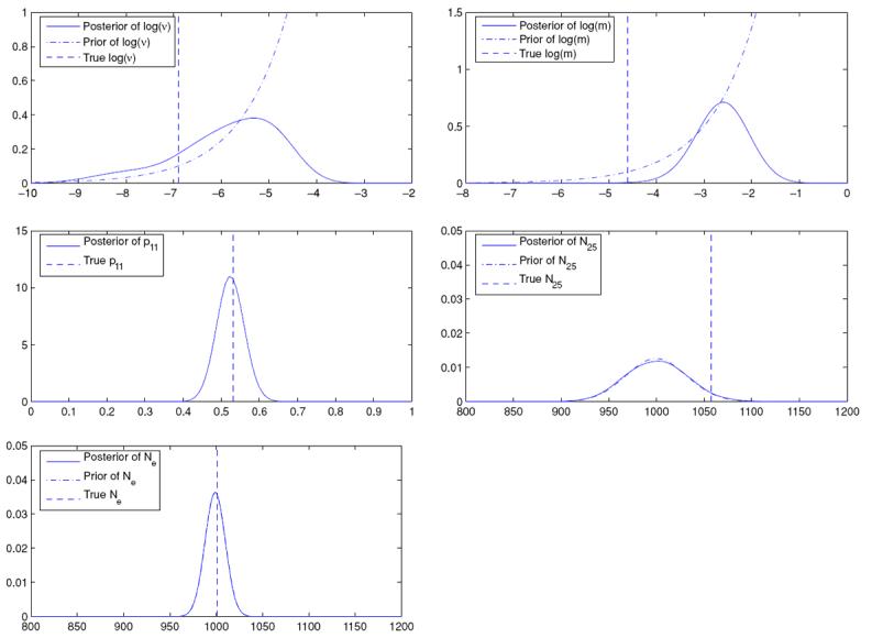
Posteriors and priors of parameters (ν and m displayed on the log scale) when the transition model is multinomial.

4.2 Example 2 : The approximate Dirichlet transition model for allele frequencies

We use the same simulated data set as in Example 1, but for inference purposes we now assume that the transition model is Dirichlet in order to test the adequacy of this approximation. The priors for the other parameters remain unchanged. The posteriors analogous to those in Figure 1 are shown in Figure 2.

Figure 2.

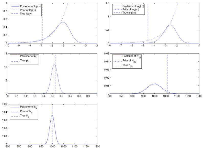
Posteriors and priors of parameters (ν and m displayed on the log scale) when the transition model is Dirichlet.

The posteriors of m, p₁₁, N₂₅ and N_e are essentially as before. The posterior of ν undergoes some change compared to Example 1; mass seems to be moved to higher mutation rates. Overall, the Dirichlet approximation seems adequate and, bearing in mind its usefulness in cases where the N_i are all equal to a common N, we adopt it in subsequent analyses.

4.3 Example 3 : Posterior inference when N_i = N

We use the same set up as in the previous examples, but assume, for data simulation as well as for inference, that N_i = N. The assumption of a common N across all populations reduces the number of parameters in the model from 102 to 53, and hence facilitates investigation on how much learning about the reduced number of parameters is possible, given the data. However, there still are more parameters than the data, so substantial learning is still not to be expected. It turns out that the posteriors of ν and m are similar to the posteriors for ν and m respectively obtained in Example 1 and so are not shown. Furthermore, due to the direct association with the data, the posteriors for the p_i always included the true values in their respective highest posterior density regions. Thus, we consider the posteriors of N, Nν and Nm. Figure 3 displays these posteriors.

Figure 3.

Posteriors of Nν, Nm and N when the transition model is Dirichlet.

From Figure 3 it can be seen that the posteriors of Nν and Nm also have the same shapes as the posteriors of ν and m of Example 1. Essentially, we have a rescaling by N; again small values of Nm receive less posterior mass. The location of posterior of N is now different from that of the prior, but the variance is almost the same as the prior, altogether only a bit more learning than in the cases where the N_i were different.

4.4 Example 4 : Effective population size – N_i are different, but assumed equal for inference

Finally, we study a case that deals with misspecification of the model. The data is simulated using the same setup as in Example 1. Specifically, N_i are allowed to vary during data simulation. However, we pretend that there is a common N across all populations. Quantities of interest are shown in Figure 4.

Figure 4.

Posteriors of Nν, Nm and N when the transition model is Dirichlet and when N_i are varying.

We notice that all the posteriors in this example are similar to those in Example 3, where N_i = N in both simulated data and inference. This is not unexpected, since learning is not substantial, as demonstrated earlier. In other words, it seems difficult for the originally different N_i to have much effect on the wrongly assumed common N. Lastly, there is no obvious connection between estimating N in this case and estimating N_e in Example 2. Though N can be viewed here as an “effective” sample size, it does not have the genetic interpretation associated with the harmonic mean in Example 2.

5 Extension to the multilocus model

In all of the examples in Section 4, we find that we learn very little about N. In this regard, what can we gain by extending the above single-locus models to models with multiple loci? Given L loci, we now observe allele frequencies p̂_lij; l = 1, … , L, i = 1, … , K and j = 1, … , A. We let p̂_li = (p̂_li1, … , p̂_liAl)′ and p_li = (p_li1, … , p_liAl)′. The sample size for population i at locus l is given by n_li. (We allow the possibility that, due to data collection issues, for a given population, the number of alleles sampled at different loci might be different.) At locus l, we denote the mutation rate by ν_l. In this case we denote by θ the parameters m and N. Here, we assume a is customary, that allele frequencies are independent across loci (see, e.g., Holsinger and Wallace (2004) and references 12 therein). Hence, the multilocus model becomes the product of L single-locus models. The form of the Bayesian model is

$$\left(\prod _{l=1}^L\prod _{i=1}^{K}f({\widehat{\mathbf{p}}}_{\mathit{li}}\mid {\mathbf{p}}_{\mathit{li}})\right)\prod _{l=1}^L\left\{f({\mathbf{p}}_{l1},\dots ,{\mathbf{p}}_{\mathit{lK}}\mid \theta ,{\nu }_l)f\left({\nu }_l\right)\right\}f\left(\theta \right)$$ (18)

From the structure of the model it is clear that θ now has information from data corresponding to all L loci. We demonstrate by simulation studies that the posteriors of m and N are indeed more informative than before.

5.1 A parallel algorithm for implementation of the multilocus problem

From (18), it is clear that the Bayesian model specifies (conditional) independence over the loci. This model is readily amenable to parallel implementation. We thus propose the following updating procedure for θ, ν₁, … , ν_L, p_l1, … , p_lK; l = 1, … , L.

• Updating ν_l for each l sequentially with a symmetric proposal density requires computation of the acceptance ratio, i.e., the ratio of f̃_B(p_l1, … , p_lK | θ, ν_l)f(ν_l), evaluated at the new and current values of ν_l respectively, other parameters remaining fixed at the current values. Here f̃_B(p_l1, … , p_lK | θ, ν_l)f(ν_l) is evaluated by exactly the same procedure discussed in Section 2.1. However, sequential evaluation of the latter for each l = 1, … , L is computationally intensive, particularly for large L. Parallelising this computation makes the procedure very efficient. Hence we propose to update mutation rates by splitting each ν_l to a different processor. At each processor, given a symmetric proposal density the new proposal will be accepted or rejected depending on the acceptance ratio, computed independently by each processor. Thus all ν_l = 1, … , L are updated simultaneously, retaining computational efficiency.

• For updating each of m and N the acceptance ratio is the ratio ${\Pi }_{l=1}^L\left\{{\tilde{f}}_B({\mathbf{p}}_{l1},\dots ,{\mathbf{p}}_{\mathit{lK}}\mid m,N,{\nu }_l)\right\}f(m,N)$, evaluated at the new and current values of m or N, other parameters fixed at the current values. We compute the acceptance ratio by first splitting the evaluation of f̃_B(p_l1, … , p_lK | m,N, ν_l) for each l into different processors. Then we combine all the factors evaluated in different processors to compute the acceptance ratio (which is done by a single processor). The decision of accepting or rejecting the proposal is then taken by this processor.

• For each l, we update p_li in a separate processor. In this case, both the proposal density and the acceptance probability are analogous to the single locus case. The conditional independence of p_li for different values of l given θ and ν₁, … , ν_L suggests that the same procedure as in the single locus case can be used to update p_li in each processor. The updating procedure within each processor may be roughly interpreted as a replication of the updating procedure in the single locus case.

5.2 Application of the methodology to simulated multilocus problems

Since it is anticipated that data from the multiple loci will help us to learn more about the parameters (the focus being on the learning about N), an obvious question is whether learning is greater when there are more loci and fewer populations or vice versa. We demonstrate below that the amount of learning is almost same in both situations.

We consider two simulated data sets, one with 10 loci, 5 populations, 2 alleles and the other with 5 loci, 10 populations and 2 alleles. We use the above algorithm on these two data sets. However, we note that acceptance rates for m and N were very small. To avoid this problem, we discretize the parameter space of m to have just three points, that is, Prob(m = 0.001, 0.01, 0.1) = 1. We also set N to have mass concentrated on four points; more explicitly, Prob(N = 50, 100, 500, 1000) = 1. Realistically, we could not expect to learn about m and N to more than roughly an order of magnitude and the above mass points are considered sensible within a population genetics setting. Thus, we do not need to use the Metropolis-Hastings step to update the parameters m and N. We place a discrete uniform prior on these values. We then associate weights with each of the mass points, the weights being proportional to the full conditional distribution given other parameters and the data, and select a mass point with probability proportional to its corresponding weight. We note here that computation of weights for each mass point involves evaluation of f̃_B(· | θ) in each case, which is computationally expensive if the number of mass points is large.

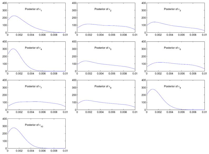
Figures 5 and 6 display the posteriors of mutation rates corresponding to the two data sets. It is seen that for both data sets, the posteriors are relatively flat. This is not unexpected, since the mutation rates are locus-specific, that is, increasing the number of loci will only increase the number of mutation rates, not the information on any mutation rate.

Figure 5.

Posteriors of ν_k; k = 1, … , 10, in the case with 10 loci and 5 populations

Figure 6.

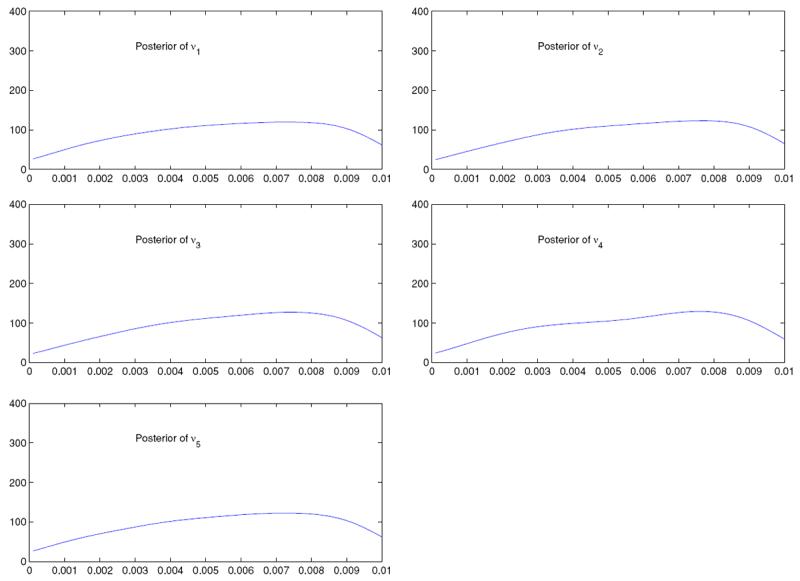
Posteriors of ν_k; k = 1, … , 5, in the case with 5 loci and 10 populations

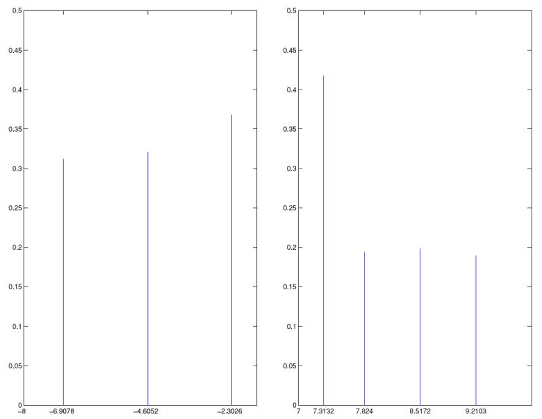
Posteriors for migration rates corresponding to the two different data sets are shown in Figure 7. In both cases, almost the entire mass of the discretized posterior is concentrated on 0.1; this indicates almost the same amount of learning about m in both cases. The concentration of the entire mass of m on 0.1 is also consistent with the single locus cases, where 0.1 gets high density. However, the true value of m, which is 0.01, receives no mass from the posterior distribution; but this is again consistent with the single locus cases.

Figure 7.

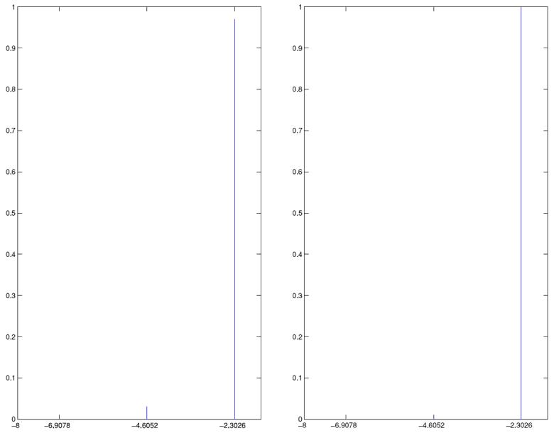
Posterior of m (displayed on the log scale); (a) corresponds to 10 loci, 5 populations and (b) corresponds to 5 loci, 10 populations

The posteriors for N corresponding to the above-explained two simulated data sets are shown in Figure 8. In both cases, it is seen that the posterior of N gives mass to only two values, 50 and 100, 50 receiving higher mass. The other two values 500 (which, incidentally, is the true value) and 1000 receive no mass at all. The above observations indicate a fair amount of learning about N, demonstrating the benefit of multilocus data. But the fact that the true value receives no mass, is in keeping with the posterior of m, which does not give mass to the true value either.

Figure 8.

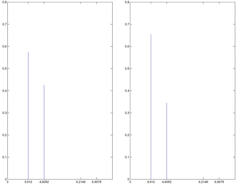
Posterior of N (displayed on the log scale); (a) corresponds to 10 loci, 5 populations and (b) corresponds to 5 loci, 10 populations.

From the simulation experiments it is also clear that there is little difference in the amount of learning of the parameters from the two data sets. However, from the viewpoint of our parallel computation algorithm, the data set with 10 loci and 5 populations is more attractive than the one with 5 loci and 10 populations. This is apparent since, given 10 loci, each can be assigned to a different processors and each such processor does the computation with 5 populations. On the other hand, with 5 loci and 10 populations, each of 5 processors does the computation with 10 populations. Given the availability of a large number of processors, the former evidently utilizes the resources much more efficiently. Specifically, to generate 10,000 realizations, implementation with 10 loci, 5 populations takes less than one hour, while implementation with 5 loci, 10 populations takes more than 2 hours.

6 Application of the methodology to a real data set

In this section we apply our proposed methodology to a human microsatellite data set with two alleles. The sampling units are 52 subpopulations (small linguistic or geographic units) within 5 broad geographic populations. For more details on the data set, see Fu et al. (2005) and the references therein. The data set consists of genotype counts which we reduce to allele counts. Also, we combined the sample counts within subpopulations into a single sample count for each geographical population. Thus, we have 5 populations and 2 alleles. There are 377 available loci but, currently, due to severe underflow and computational stability problems we are unable to achieve reliable estimation of the required density f̃_B(p₁, … , p_K | θ) using all of these loci. Possible remedies are the subject of a future manuscript but, for the present purpose, we provide an illustrative analysis based on 10 randomly chosen loci from the set of 377.

The posteriors for ν_l; l = 1, … , 10, m and N are shown in Figures 9 and 10. In essence, the posteriors are in keeping with those corresponding to the simulated data sets. However, there are notable differences. For example, Figure 9 shows that the posterior of several migration rates are more informative than those corresponding to the simulated data sets. The mode of the posterior of m is again seen to be 0.1, as in the simulated data case, but the other points also receive significant mass, unlike in the simulated data case. The smallest value of N turns out to be the mode of the posterior of N as in the simulation experiments, but in this case other points receive more mass compared to the simulation experiments. Indeed, for m and N there is little Bayesian learning.

Figure 9.

Posteriors of ν_k; k = 1, … , 10 using the human microsatellite data (see Section 6 for details).

Figure 10.

(a) Posterior of m and (b) posterior of N (both displayed on the log scale) using the human microsatellite data (see Section 6 for details)

7 Other ecological applications

We briefly describe two other ecological settings that are driven by a LEP. In Section 7.1 we consider a community biodiversity illustration due to Hubbell (Hubbell (2001), McKane et al. (2004)). In Section 7.2 we turn to a habitat dynamics example (Hanski (1994), Molainen and Hanski (1998)).

7.1 Hubbell's neutral theory of community biodiversity

Assume at time t that there are N_i(t) individuals of species i in the local community and let ${\Sigma }_{i=1}^r{N}_i\left(t\right)=J$ for all t, where r is the total number of species in the local community. The transition from time t to time t + 1 selects one individual from the community at random and replaces it with another individual drawn either from the local community with probability 1 – m or from a regional metacommunity with probability m. When drawing an individual from the metacommunity we select one of species i with probability P_i. Thus,

$$\begin{array}{cc}\hfill P(N_i(t+1)=k_i-1\mid N_i\left(t\right)=k_i)=& (1-m)\frac{N_i}{J}\frac{J-N_i}{J-1}+m\frac{N_i}{J}(1-P_i)\hfill \\ \hfill P(N_i(t+1)=k_i\mid N_i\left(t\right)=k_i)=& 1-(1-m)\frac{N_i}{J}\frac{J-N_i}{J-1}-m\frac{N_i}{J}(1-P_i)\hfill \\ \hfill & -(1-m)\frac{J-N_i}{J}\frac{N_i}{J-1}-m\frac{J-N_i}{J}{P}_i\hfill \\ \hfill P(N_i(t+1)=k_i+1\mid N_i\left(t\right)=k_i)=& (1-m)\frac{J-N_i}{J}\frac{N_i}{J-1}+m\frac{J-N_i}{J}{P}_i\hfill \end{array}$$

An explicit (approximate) solution for the stationary distribution of this process, f(N^(t) | P, J, m) is possible using an appropriate continuous approximation. Interest in this model focuses on estimating m and J (Latimer et al. (2005)).

The data consist of s samples collected at the same time from different parts of what is assumed to be the same metacommunity, where there are S_is individuals of species i in sample s. S_s, the vector of abundances in sample s, is hypergeometric with parameters N_s and sample size T_s = Σ_i S_is. With priors on P, J, and m, the specification of the LEP model is complete.

7.2 Incidence function models in metapopulation dynamics

Populations occupy distinct patches of habitat. Let $p_i^{\left(t\right)}=1$ if patch i is occupied at time t and $p_i^{\left(t\right)}=0$ if it is unoccupied. Let M be the transition matrix for a Markov chain that describes the dynamics of $p_i^{\left(t\right)}$.

$$\mathbf{M}=\left(\begin{array}{cc}\hfill 1-C_i\left(t\right)\hfill & \hfill C_i\left(t\right)\hfill \\ \hfill E_i\left(t\right)\hfill & \hfill 1-E_i\left(t\right)\hfill \end{array}\right)$$

where C_i(t) is the probability that patch i will be colonized at time t+1 if patch i is unoccupied at time t ($p_i^{\left(t\right)}=0$ and $p_i^{(t+1)}=1$) and E_i(t) is the probability that the population at patch i goes extinct given that it is present at time t ($p_i^{\left(t\right)}=1$ and $p_i^{(t+1)}=0$). Suppose

$$\begin{array}{cc}\hfill E_i\left(t\right)& =\min \left(\frac{\mu }{A_i^x},1\right)\hfill \\ \hfill C_i\left(t\right)& =\frac{M_i^2\left(t\right)+{\gamma }_1}{M_i^2\left(t\right)+{\gamma }_1+{\gamma }_2}\hfill \\ \hfill M_i\left(t\right)& =\beta \underset{j}{\Sigma }{p}_j^{\left(t\right)}{e}^{-\alpha d_{\mathit{ij}}}{A}_j,\hfill \end{array}$$

where A_i is the area of patch i and d_ij is the distance between patch i and patch j. θ = (μ, x, α, β, γ₁, γ₂) is the vector of model parameters.

The data consist of observations on patch occupancy (presence or absence of a population) and patch areas. Specifically, Y_i = 1 if patch i is occupied when observed, so Y_i ∼ Bernoulli(p_i). Then, collecting the Y_i's and p_i's into vectors Y and p, the LEP model is f(p, θ | Y) ∝ f(Y | p)f(p | θ)f(θ).

8 Discussion

This paper has focused on model fitting strategies for what we have called latent equilibrium process models. While suggesting a range of potential applications, we have concentrated on population genetics models. In particular, we have investigated the case of two alleles with constant mutation and migration rates. In principle, our proposed methodology can be extended to accommodate general migration and mutation matrices and to arbitrary number of populations and alleles though substantial computational challenges will ensue.

Also, with a single locus, little learning would be anticipated. However, as in this paper, learning may be improved by incorporating data from multiple loci. But the speed of the MCMC algorithm may remain an issue. For instance, under fully general mutation and migration matrices, noting that the columns of each matrix are dependent (since the rows sum to one), it will be necessary to update the mutation vector (ν_r1, … , ν_r,A)′ and the migration vector (m_r1, … , m_r,K)′ sequentially for each population r = 1, … , K. This implies that the number of evaluations of f̃_B(· | θ) in a single iteration will be the same as the number of rows of the migration matrix and and the number of rows of the mutation matrix. For a large number of populations the difficulties are evident. Also, since it is necessary to update all elements of each row of each of the migration and the mutation matrices simultaneously, in the case of many more than two of alleles, the (Metropolis) acceptance rate of the vectors may be very low. In summary, the methodology we have proposed seems to be the most promising way currently available to attack the fitting of the general class of models that are our interest. However, much computational refinement is still required in order to adequately handle the level of generality we seek.

9 Appendix: Simulation study

We consider a simulation study to demonstrate the validity of our theoretical assertion regarding convergence of our MCMC algorithm.

Given a data set of the form Y = (y₁, … , y_n)′, we consider a Bayesian model of the form ${\Pi }_{i=1}^{n}f(y_i\mid \theta )f\left(\theta \right)$. In particular, we assume that, f(y_i | θ) is a normal density with mean θ and variance 1, and that f(θ) is the stationary distribution corresponding to a Markov chain with three states, whose transition matrix is a reflecting barrier of the form

$$P=\left(\begin{array}{ccc}\hfill p\hfill & \hfill q\hfill & \hfill 0\hfill \\ \hfill 0\hfill & \hfill p\hfill & \hfill q\hfill \\ \hfill q\hfill & \hfill 0\hfill & \hfill p\hfill \end{array}\right)$$

Hence, the stationary probability of each of the three states of θ is 1/3. In other words, the prior f(θ) is uniform, with probability 1/3 for each value of θ. For this toy LEP model we choose n = 10, p = q = 1/2, and the 3 states of θ as 0, 0.1 and 0.2. Given the data set Y = (−0.4412, −1.2335, 1.1727, −0.6121, 0.0887, 0.0992, −0.1494, 0.4966, −0.1640, −1.5640)′ the exact posterior probabilities for the three states are then given by 0.4403, 0.3325 and 0.2272 respectively.

Now, assuming that the stationary distribution of f(θ) is unknown, and that only the transition model, which, here, is the reflecting barrier, is known, we implement our proposed MCMC algorithm on this LEP model. In particular, we propose θ by running the transition model to stationarity at each iteration. Thus,

$${\tilde{f}}_B(\theta =x)=\frac{1}{B}\underset{t=1}{\overset{B}{\Sigma }}f(\theta =x\mid z^{\left(t\right)})$$

is the estimated stationary distribution of θ, where {z_t; t = 1, … , B} are obtained by running the transition model to stationarity, for sufficiently large B. Since f̃_B(θ = x) is expected to approximate f(θ) arbitrarily well, we recognise

$$\beta =\min \left\{1,\frac{\prod _{i=1}^{n}f(y_i\mid {\theta }^{\left(\mathit{new}\right)})}{\prod _{i=1}^{n}f(y_i\mid {\theta }^{\left(\mathit{curr}\right)})}\right\}$$

as the acceptance probability of θ.

Choosing B = 1000, discarding the first 5000 samples as burn-in and storing 1 out of 5 samples in the next 25000 samples generated, giving a total of 5000 realizations of θ, we obtain the approximate probabilities of the states 0, 0.1 and 0.2 as 0.4438, 0.3326 and 0.2236 respectively.

The results clearly demonstrate the validity of our proposed MCMC method for LEP models and supports our theoretical results.

References

- Beerli P, Felsenstein J. Maximum-likelihood estimation of migration rates and effective population numbers in two populations using a coalescent approach. Genetics. 1999;152:763–773. doi: 10.1093/genetics/152.2.763. [DOI] [PMC free article] [PubMed] [Google Scholar]
- Berliner LM. Hierarchical Bayesian time series models. In: Hanson K, Silver R, editors. Maximum Entropy and Bayesian Methods. Kluwer Academic Publishers; Dordrecht, Netherlands: 1996. pp. 15–22. [Google Scholar]
- Clark JS, Ferraz G, Oguge N, Hays H, DiCostanzo J. Hierarchical Bayes for Structured, Variable Populations: from Recapture Data to Life-History Prediction. Ecology. 2005;86(8):2232–2244. [Google Scholar]
- Crow JF, Kimura M. An Introduction to Population Genetics Theory. Burgess Publishing Company; Minneapolis: 1970. [Google Scholar]
- Donnelly P, Tavare S. Coalescents and genealogical structure under neutrality. Annual Reviews of Genetics. 1995;29:401–421. doi: 10.1146/annurev.ge.29.120195.002153. [DOI] [PubMed] [Google Scholar]
- Doucet A, de Freitas N, Gordon N. Sequential Monte Carlo Methods in Practice. Springer-Verlag; New York: 2001. [Google Scholar]
- Ewens WJ. Mathematical Population Genetics. Springer-Verlag; Berlin: 1979. [Google Scholar]
- Fu R, Dey D, Holsinger KE. Bayesian models for the analysis of genetic structure when populations are correlated. Bioinformatics. 2005;21(8):1516–1529. doi: 10.1093/bioinformatics/bti178. [DOI] [PubMed] [Google Scholar]
- Fu R, Gelfand AE, Holsinger KE. Exact moment calculations for genetic models with migration, mutation, and drift. Theoretical Population Biology. 2003;63:231–243. doi: 10.1016/s0040-5809(03)00003-0. [DOI] [PubMed] [Google Scholar]
- Hanski I. A practical model of metapopulation dynamics. Journal of Animal Ecology. 1994;63:151–162. [Google Scholar]
- Holsinger KE, Wallace LE. Bayesian approaches for the analysis of population genetic structure: an example from Platanthera leucophaea (Orchidaceae) Molecular Ecology. 2004;13:887–894. doi: 10.1111/j.1365-294x.2004.02052.x. [DOI] [PubMed] [Google Scholar]
- Hubbell SP. The Unified Neutral Theory of Biodiversity and Biogeography. Princeton University Press; Princeton: 2001. [Google Scholar]
- Kalnay E. Atmospheric Modelling, Data Assimilation and Predictability. Cambridge University Press; Cambridge: 2003. [Google Scholar]
- Karlin S. Rates of approach to homozygosity for finite stochastic models with variable population size. The American Naturalist. 1968;102:443–455. [Google Scholar]
- Latimer AM, Silander JA, Jr., Cowling RM. Neutral ecological theory reveals isolation and rapid speciation in a biodiversity spot. Science. 2005;309:1722–1725. doi: 10.1126/science.1115576. [DOI] [PubMed] [Google Scholar]
- Liu J. Monte Carlo Strategies in Scientific Computing. Springer-Verlag; New York: 2001. [Google Scholar]
- McKane AJ, Alonso D, Solé RV. Analytic solution of Hubbel's model of local community dynamics. 2004 doi: 10.1016/j.tpb.2003.08.001. [DOI] [PubMed] [Google Scholar]
- Meyn SP, Tweedie RL. Markov Chains and Stochastic Stability. Springer-Verlag; London: 1993. [Google Scholar]
- Molainen A, Hanski I. Metapopulation dynamics: effects of habitat quality and landscape structure. Ecology. 1998;79:2503–2515. [Google Scholar]
- Nummelin E. General Irreducible Markov Chains and Non-negative Operators. Cambridge University Press; London: 1984. [Google Scholar]
- Shugart HH. How the Earthquake Bird Got its Name and Other Tales of an Unbalanced Nature. Yale University Press; New Haven: 2004. [Google Scholar]
- Song S, Dey DK, Holsinger KE. Differentiation among populations with migration, mutation, and drift: implications for genetic influence. Evolution. 2005 in press. [PMC free article] [PubMed] [Google Scholar]
- Turchin P. Complex Population Dynamics: A theoretical/empirical synthesis. Princeton University Press; Princeton: 2003. [Google Scholar]
- Wikle CK, Berliner LM, Cressie NAC. Hierarchical Bayesian space-time models. Journal of Environmental and Ecological Statistics. 1998;14(5):117–154. [Google Scholar]