Methods for testing theory and evaluating impact in randomized field trials

Abstract

Randomized field trials provide unique opportunities to examine the effectiveness of an intervention in real world settings and to test and extend both theory of etiology and theory of intervention. These trials are designed not only to test for overall intervention impact but also to examine how impact varies as a function of individual level characteristics, context, and across time. Examination of such variation in impact requires analytical methods that take into account the trial’s multiple nested structure and the evolving changes in outcomes over time. The models that we describe here merge multilevel modeling with growth modeling, allowing for variation in impact to be represented through discrete mixtures—growth mixture models—and nonparametric smooth functions—generalized additive mixed models. These methods are part of an emerging class of multilevel growth mixture models, and we illustrate these with models that examine overall impact and variation in impact. In this paper, we define intent-to-treat analyses in group-randomized multilevel field trials and discuss appropriate ways to identify, examine, and test for variation in impact without inflating the Type I error rate. We describe how to make causal inferences more robust to misspecification of covariates in such analyses and how to summarize and present these interactive intervention effects clearly. Practical strategies for reducing model complexity, checking model fit, and handling missing data are discussed using six randomized field trials to show how these methods may be used across trials randomized at different levels.

1. Introduction

Randomized field trials (RFTs) provide a powerful means of testing a defined intervention under realistic conditions. Just as important as the empirical evidence of overall impact that a trial provides (Flay et al., 2005), an RFT can also refine and extend both etiologic theory and intervention theory. Etiologic theory examines the role of risk and protective factors in prevention, and an RFT formally tests whether changes in these hypothesized factors lead to the prevention of targeted outcomes. Theories of intervention characterize how change in risk or protective factors impact immediate and distal targets and how specific theory driven mediators produce such changes (Kellam and Rebok, 1992; Kellam et al., 1999). The elaborations in theory that can come from an RFT draw on understanding the interactive effects of individual level variation in response over time to different environmental influences. An adolescent drug abuse prevention program that addresses perceived norms, for example, may differentially affect those already using substances compared to nonusers. This intervention’s effect may also differ in schools that have norms favoring use compared to schools with norms favoring nonuse. Finally, the impact may differ in middle and high school as early benefits may wane or become stronger over time.

This paper presents a general analytic framework and a range of analytic methods that characterize intervention impact in RFTs that may vary across individuals, contexts, and time. The framework begins by distinguishing the types of research questions that RFTs address, then continues by introducing a general three-level description of RFT designs. Six different RFTs are described briefly in terms of these three levels, and illustrations are used to show how to test theoretically driven hypotheses of impact variation across persons, place, and time. In this paper, we focus on intent-to-treat (ITT) analyses that examine the influence of baseline factors on impact, and leave all post-assignment analyses, such as mediation analysis, for discussions elsewhere. This separation into two parts is for pragmatic and space considerations only, as post-assignment analyses provide valuable insights into ITT results and are generally included in major evaluations of impact. For these intent-to-treat analyses, we present standards for determining which subjects should be included in analyses, how missing data and differences in intervention exposure should be handled, and what causal interpretations can be legitimately drawn from the statistical summaries. We present the full range of different modeling strategies available for examining variation in impact, and we emphasize those statistical models that are the most flexible in addressing individual level and contextual factors across time. Two underutilized methods for examining impact, generalized additive mixed models (GAMM) and growth mixture models (GMM), are presented in detail and applied to provide new findings on the impact of the Good Behavior Game (GBG) in the First Generation Baltimore Prevention Program trial.

We first define a randomized field trial and then describe the research questions it answers. An RFT uses randomization to test two or more defined psychosocial or education intervention conditions against one another in the field or community under realistic training, supervision, program funding, implementation, and administration conditions. All these conditions are relevant to evaluating effectiveness or impact within real world settings (Flay, 1986). In contrast, there are other randomized trials that test the efficacy of preventive interventions in early phases of development. These efficacy trials are designed to examine the maximal effect under restricted, highly standardized conditions that often reduce individual or contextual variation as much as possible. Testing efficacy requires that the intervention be implemented as intended and delivered with full fidelity. The interventions in efficacy trials are delivered by intervention agents (Snyder et al., 2006) who are carefully screened and highly trained. In efficacy trials, they are generally professionals who are brought in by an external research team. By contrast, the intervention agents of RFTs are often parents, community leaders, teachers or other practitioners who come from within the indigenous community or institutional settings (Flay, 1986). The level of fidelity in RFTs is thus likely to vary considerably, and examining such variation in delivery can be important in evaluating impact (Brown and Liao, 1999). Both types of trials are part of a larger strategy to build new interventions and test their ultimate effects in target populations (Greenwald and Cullen, 1985).

As a special class of experiments, RFTs have some unique features. Most importantly, they differ from efficacy trials on the degree of control placed on implementation of the intervention. They are designed to address questions other than those of pure efficacy, and they often assess both mediator and moderator effects (Krull and MacKinnon, 1999; MacKinnon and Dwyer, 1993; MacKinnon et al., 1989; Tein et al., 2004). Also, they often differ from many traditional trials by the level at which randomization occurs as well as the choice of target population. These differences are discussed below starting with comments on program implementation first.

Program implementation is quite likely to vary in RFTs due to variation in the skills and other factors that may make some teachers or parents more able to carry out the intervention than others even when they receive the same amount of training. These trials are designed to test an intervention the way it would be implemented within its community, agency, institutional, or governmental home setting. In such settings, differences in early and continued training, support for the implementers, and differences in the aptitude of the implementers can lead to variation in implementation. The intervention implementers, who are typically not under the control of the research team the way they are in efficacy trials, are likely to deliver the program with varied fidelity, more adaptation, and less regularity than that which occurs in efficacy trials (Dane and Schneider, 1998; Domitrovich and Greenberg, 2000; Harachi et al., 1999). Traditional intent-to-treat analyses which do not adjust for potential variations in implementation, fidelity, participation, or adherence, are often supplemented with “as-treated” analyses, mediation analysis, and other post-assignment analyses described elsewhere (Brown and Liao, 1999; Jo, 2002; MacKinnon, 2006).

A second common difference between RFTs and controlled efficacy trials is that the intervention often occurs at a group rather than individual level; random assignment in an efficacy trial is frequently at the level of the individual while that for an RFT generally occurs at levels other than the individual, such as classroom, school, or community. Individuals assigned to the same intervention cluster are assessed prior to and after the intervention, and their characteristics, as well as characteristics of their intervention group may serve in multilevel analyses of mediation or moderation (Krull and MacKinnon, 1999). In addition, levels nested above the group level where intervention assignment occurs, such as the school in a classroom randomized trial, can also be used in assessing variation in intervention impact. Examples of six recent multilevel designs are presented in Table 1; these are chosen because random assignment occurs at different levels ranging from the individual level to the classroom, school, district, and county level. This table describes the different levels in each trial as well as the individual level denominators that are used in intent-to-treat analyses, a topic we present in detail in Section 2.2. We continue to refer to these trials in this paper to illustrate the general approach to analyzing variation in impact for intent-to-treat, as treated, and other analyses involving post-assignment outcomes.

Table 1.

Design factors at the individual, group, and block level and covariates hypothesized to account for variation in intervention impact for six randomized field trials

Level where intervention assignment occurs (trial name/sponsor)	Active intervention arms	Individual level sample and intent-to-treat denominators	Level where intervention assignment occurs	Level of blocking
	Goal	Predicted impact	Predicted impact
1. Individual Level Random Assignment (Rochester Resilience Program/NIMH (RRP))	Promoting Resilient Children Initiative (PRCI) delivered by school-based mentors to 1st-3rd graders and their parents	470 1st-3rd graders with behavioral or learning problems	Individual level assignment within classroom to school-based mentor or control condition	75 classrooms in 5 schools in 1 district
	Goal: reduce internalizing and externalizing problems	Impact predicted to vary by level of child risk at baseline	Impact predicted to vary by grade level, teacher, mentor, and school factors
2. Classroom level random assignment (First Generation Baltimore Prevention Program/NIMH NIDA (First BPP Trial))	Good behavior game, mastery learning classroom-based interventions	1196 1st graders who were present when initial assessments were made	41 classrooms	19 schools in 5 geographic areas
	Goal: promote behavior and learning, success in school, and long-term prevention of drug use and externalizing behavior	Impact predicted to vary by individual aggressive, disruptive behavior at beginning of first grade	Impact predicted to vary by average classroom aggressive, disruptive behavior at baseline	Impact predicted to vary by school and urban factors
3. Individual and classroom level random assignment (Third Generation Baltimore Prevention Program Whole Day /NIDA (Third Generation BPP Trial))	Whole day classroom intervention aimed at teachers to improve reading instruction, classroom management, and parent involvement	First graders randomly assigned to classroom within school whenever they enter throughout year	One of two classrooms randomly assigned to intervention in each of 12 schools	12 elementary schools
	Goal: improve achievement and reduce aggressive, disruptive behavior, and long-term impact on drug use and externalizing behaviors	Impact predicted to vary by child achievement and aggressive, disruptive behavior at baseline	Impact predicted to vary by baseline teaching performance and behavior management	Impact predicted to vary by school factors
4. School level randomization (Georgia Gatekeeper Program/NIMH (GA Gatekeeper Trial))	Training of all school staff in QPR citizen gatekeeper	50,000 Students who were enrolled in one of the 32 schools at the beginning of the year. A stratified random sample of school staff in these schools, assigned according to their placement at beginning of school year	20 middle and 12 high schools randomly assigned different times of training	One school district
	Goal: increase identification of suicidal youth by school staff	Impact predicted to vary by gender, grade level, race/ethnicity	Impact predicted to vary by staffs’ average referral behavior on baseline attitudes and behavior	Not applicable
5. School district randomization (Adolescent Substance Abuse Prevention Study/RW Johnson (ASAPS))	New DARE Program in 7th and 9th Grades	18,000 7th Graders initially enrolled in one of the school districts	84 school districts	6 geographic regions
	Goal: prevent adolescent substance use/abuse	Impact predicted to vary by baseline risk status	Impact predicted to vary by school norms and sociodemographics	Impact predicted to vary by geographic region
6. County level randomization (California Multidimensional Treatment Foster Care (MTFC) Trial/NIMH (CA MTFC))	Community Development Team (CDT) vs. Standard Condition for Implementation	Family Mental Health Agencies and County Directors. Foster Care Families in these counties; none available for intent-to-treat analyses	40 Counties randomized to timing and type of implementation	1 State
	Goal: increase full implementation of MTFC at the county level through peer-to-peer cross-county program	Impact predicted to vary by role in county implementation	Impact predicted to vary by static county characteristics

Finally, RFTs often target heterogeneous populations, whereas controlled experiments routinely use tight inclusion/exclusion criteria to test the intervention with a homogenous group. Because they are population-based, RFTs can be used to examine variation in impact across the population, for example to understand whether a drug prevention program in middle school has a different impact on those who are already using substances at baseline compared to those who have not yet used substances. This naturally offers an opportunity to examine the impact by baseline level of risk, and thereby examine whether changes in this risk affect outcomes in accord with etiologic theory.

We are often just as interested in examining variation in impact in RFTs as we are in examining the main effect. For example, a universal, whole classroom intervention aimed proximally at reducing early aggressive, disruptive behavior and distally at preventing later drug abuse/dependence disorders may impact those children who were aggressive, disruptive at baseline but have little impact on low aggressive, disruptive children. It may work especially well in classes with high numbers of aggressive, disruptive children but show less impact in either classrooms with low numbers of aggressive, disruptive children or in classrooms that are already well managed. Incorporating these contextual factors in multilevel analyses should also increase our ability to generalize results to broader settings (Cronbach, 1972; Shadish et al., 2002). Prevention of or delay in later drug abuse/dependence disorders may also depend on continued reduction in aggressive, disruptive behavior through time. Thus our analytic modeling of intervention impact or RFTs will often require us to incorporate growth trajectories, as well as multilevel factors.

RFTs, such as that of the Baltimore Prevention Program (BPP) described in this issue of Drug and Alcohol Dependence (Kellam et al., 2008), are designed to examine the three fundamental questions of a prevention program’s impact on a defined population: (1) who benefits; (2) for how long; (3) and under what conditions or contexts? Answering these three questions allows us to draw inferences and refine theories of intervention far beyond what we could do if we only address whether a significant overall program impact was found. The corresponding analytical approaches we use to answer these questions require greater sophistication and model checking than would ordinarily be required of analyses limited to addressing overall program impact. In this paper, we present integrative analytic strategies for addressing these three general questions from an RFT and illustrate how they test and build theory as well as lead to increased effectiveness at a population level. Appropriate uses of these methods to address specific research questions are given and illustrated on data related to the prevention of drug abuse/dependence disorders from the First Baltimore Prevention Program trial and other ongoing RFTs.

The prevention science goal in understanding who benefits, for how long, and under what conditions or contexts draws on similar perspectives from both theories of human behavior and from methodology that characterize how behaviors change through time and context. In the developmental sciences, for example, the focus is on examining how individual behavior is shaped over time or stage of life by individual differences acting in environmental contexts (Weiss, 1949). In epidemiology, which seeks to identify the causes of a disorder in a population, we first start descriptively by identifying the person, place, and time factors that link those with the disorder to those without such a disorder (Lilienfeld and Lilienfeld, 1980).

From the perspective of prevention methodology, these same person, place, and time considerations play a fundamental roles in trial design (Brown and Liao, 1999; Brown et al., 2006, 2007a,b) and analysis (Brown et al., 2008; Bryk and Raudenbush, 1987; Goldstein, 2003; Hedeker and Gibbons, 1994; Muthén, 1997; Muthén and Shedden, 1999; Muthén et al., 2002; Raudenbush, 1997; Wang et al., 2005; Xu and Hedeker, 2001). Randomized trial designs have extended beyond those with individual level randomization to those that randomize at the level of the group or place (Brown and Liao, 1999; Brown et al., 2006; Donner and Klar, 2000; Murray, 1998; Raudenbush, 1997; Raudenbush and Liu, 2000; Seltzer, 2004). Randomization also can occur simultaneously in time and place as illustrated in dynamic wait-listed designs where schools are assigned to receive an intervention at randomly determined times (Brown et al., 2006). Finally, in a number of analytic approaches used by prevention methodologists that are derived from the fields of biostatistics, psychometrics, and the newly emerging ecometrics (Raudenbush and Sampson, 1999), there now exist ways to include characteristics of person and place in examining impact through time.

There has been extensive methodologic work done to develop analytic models that focus on person, place, and time. For modeling variation across persons, we often use two broad classes of modeling. Regression modeling is used to assess the impact of observed covariates that are measured on individuals and contexts that are measured without error. Mixed effects modeling, random effects, latent variables, or latent classes are used when there is important measurement error, when there are unobserved variables or groupings, or when clustering in contexts produces intraclass correlation. For modeling the role of places or context, multilevel modeling or mixed modeling is commonly used. For models involving time, growth modeling is often used, although growth can be examined in a multilevel framework as well. While all these types of models—regression, random effects, latent variable, latent class, multilevel, mixed, and growth modeling—have been developed somewhat separately from one another, the recent trend has been to integrate many of these perspectives. There is a growing overlap in the overall models that are available from these different perspectives (Brown et al., 2008; Gibbons et al., 1988), and direct correspondences between these approaches can often be made (Wang et al., 2005). Indeed, the newest versions of many well-known software packages in multilevel modeling (HLM, MLWin), mixed or random effect modeling (SAS, Splus, R, SuperMix), and latent variable and growth modeling (Mplus, Amos), provide routines that can replicate models from several of the other packages.

Out of this new analytic integration come increased opportunities for examining complex research questions that are now being raised by our trials. In this paper, we provide a framework for carrying out such analyses with data from RFTs in the pursuit of answers to the three questions of who benefits, for how long, and under what conditions or contexts. In Section 2, we describe analytic and modeling issues to examine impact of individual and contextual effects on a single outcome measure. In this section, we deal with defining intent-to-treat analyses for multilevel trials, handling missing data, theoretical models of variation in impact, modeling and interpreting specific estimates as causal effects of the intervention, and methods for adjusting for different rates of assignment to the intervention. The first model we describe is a generalized linear mixed model (GLMM), which models a binary outcome using logistic regression and includes random effects as well. We conclude with a discussion of generalized additive mixed models, which represent the most integrative model in this class. Some of this section includes technical discussion of statistical issues; non-technical readers can skip these sections without losing the meaning by attending to the concluding sentences that describe the findings in less technical terms, as well as the examples and figures.

In Section 3, we discuss methods to examine intervention impact on growth trajectories. We discuss representing intervention impact in our models with specific coefficients that can be tested. Because of their importance to examining the effects of prevention programs, growth mixture models are highlighted, and we provide a causal interpretation of these parameters as well as discuss a number of methods to examine model fit. Again, non-technical readers can skip the equations and attend to introductory statements that precede the technical discussions.

Section 4 returns to the use of these analyses for testing impact and building theory. We also describe newer modeling techniques, called General Growth Mixture Models (GGMM), that are beginning to integrate the models described in Sections 2 and 3.

2. Using an RFT to determine who benefits from or is harmed by an intervention on a single outcome measure

This question is centrally concerned with assessing intervention impact across a range of individual, group, and context level characteristics. We note first that population-based randomized preventive field trials have the flexibility of addressing this question much more broadly than do traditional clinicbased randomized trials where selection into the clinic makes it hard to study variation in impact. With classic pharmaceutical randomized clinical trials (P-RCT’s), the most common type of controlled experiment in humans, there is a well accepted methodology for evaluating impact that began with the early pharmacotherapy trials conducted by A. B. Hill starting in the 1940s (Hill, 1962) and is now routinely used by pharmaceutical licensing agencies such as the U.S. Food and Drug Administration and similar agencies in Europe and elsewhere. The most important impact analysis for P-RCTs has been the so-called “intent-to-treat” (ITT) analysis, a set of rigid rules that determine (1) who is included in the analyses—the denominator—(2) how to classify subjects into intervention conditions, and (3) how to handle attrition. ITT is also intended to lead to a conservative estimate of intervention impact in the presence of partial adherence to a medication and partial dropout from the study during the follow-up period (Lachin, 2000; Lavori, 1992; Pocock, 1983; Tsiatis, 1990). These two sources of bias, called treatment dropout and study dropout (Kleinman et al., 1998), have direct analogues in RFTs as well (Brown and Liao, 1999). Detailed examination of how these two factors impact statistical inferences in RCTs have been done by others (Kleinman et al., 1998). In this paper, we use a minimum of technical language to examine first the accepted characteristics of ITT analyses for P-RCTs and then specify a new standard for multilevel RFTs directed at our interests in understanding variation of impact among individuals, places, and time.

2.1. Intent-to-treat analyses for pharmaceutical randomized controlled trials

For standard clinic-based trials, ITT analyses define the denominator to include all those who have been randomly assigned, regardless of level of treatment received. ITT analyses specifically include those who agree to be randomized but then refuse to start on their assigned treatment. The often stated logic of making no exclusions based on post-assignment information, including treatment adherence, is that the alternative subgroup analyses that are formed by deleting subjects based on their adherence behavior after randomization could make the resulting treatment and control subjects unequal. Those who are failing to respond may leave treatment disproportionately more often compared to those who respond well or like the treatment (Kleinman et al., 1998; Tsiatis, 1990). Later, we will discuss this same principle in specifying ITT analysis of RFTs.

Secondly, the denominator in ITT analyses in P-RCTs includes those who complete the study as well as those who drop out, cannot be located, or refuse to be interviewed at one or more follow-up times. This decision maintains the comparability of the treatment groups that were randomized at baseline. Other alternative choices of the denominator, e.g., limiting analyses to only those who have full follow-up, would lead to unequal treatment groups if, for example, those who died were excluded from the analysis. Indeed, if survival were higher in the treated group than in the control, then a comparison of the health status of survivors alone could easily lead to an erroneous conclusion that outcomes on a drug that saved lives were worse than those on placebo.

The inclusion of all subjects in ITT analyses regardless of their follow-up status requires us to deal with the resulting missing data. For handling missing longitudinal data in ITT analyses, several approaches are used. The most common approach is the replacement of each subject’s missing data with his or her last non-missing observation, a method called last observation carried forward (LOCF). While LOCF is still the preferred method for handling longitudinal missing data when submitting drug studies to the FDA, this method is not only inefficient from a statistical point of view but also is known to introduce bias in estimates and their standard errors and at times to be misleadingly precise as well (Gibbons et al., 1988; Mazumdar et al., 1999). Most statisticians recommend against the use of LOCF (Little and Rubin, 1987; Little and Yau, 1996), and our recommendation for handling missing data in RFTs reflects this as well.

A final specification about ITT analyses in P-RCTs is that treatment assignment is based on the originally assigned—intended—treatment, rather than the treatment actually received, regardless of whether the assigned medication or placebo actually was taken. There are both practical and statistical reasons for using this strict classification rule (Kleinman et al., 1998), which clearly attenuates the estimate of intervention impact when some subjects take little or no medication. The conservative nature of the ITT analysis is thought to be more in line with the effects one would actually see in a population that will not likely maintain perfect adherence. Alternative “as-treated” (AT) analyses that take into account actual treatment received, dosage, and selection factors are all subject to assumptions that often are not verifiable, and are thus used to supplement, not replace an ITT analysis (e.g., Jo, 2002; Jo and Muthén, 2001; Wyman et al., in press).

2.2. Standards for intent-to-treat analyses for randomized field trials

Intent-to-treat analyses in RFTs serve the same purpose as that for P-RCTs. They provide an objective method of conducting analyses of impact based on comparable groups of subjects across intervention condition without regard to post-assignment information such as the dosage actually received (see Kellam et al., 2008, for example). These ITT analyses are designed to provide conservative estimates of intervention impact and may be supplemented by other analyses that examine impact on individuals “as treated” or stratified by intervention adherence (e.g.,Jo, 2002; Jo and Muthén, 2001; Wyman et al., in press).

In this section, we specify a new set of standards for conducting ITT analyses for multilevel RFTs. These standards address: (1) the denominator, or which subjects should be included or excluded in the ITT analysis; (2) how to assign subjects to the appropriate intervention group when there is mobility across intervention conditions; and (3) how to handle missing longitudinal data resulting from entrances, exits, and other reasons for missed assessments. Because an ITT analysis requires care in defining the appropriate individual level denominator, this has implications for trial design after the conclusion of the intervention period into the follow-up period (Brown and Liao, 1999; Brown et al., 2000).

2.2.1. Defining denominators for ITT analyses in group-randomized field trials

In multilevel randomized trial designs, individuals are nested in contexts such as classrooms, schools, and/or neighborhoods. One or more of these higher levels also serve as units of assignment of the intervention. For example, the First Generation Baltimore Prevention Program trial, described in the second row of Table 1, involved 41 first-grade classrooms in 19 elementary schools (Brown et al., 2007a; Kellam et al., 2008). Thus, defining a denominator for an ITT analysis first requires defining which of these first-grade classrooms should be included in the analysis, then which students should be included based on their assignment to these classrooms.

2.2.1.1. Denominator at the level of randomization for ITT analyses

Because there will necessarily be a stated protocol for assigning units to intervention based on a randomization scheme, determining the appropriate denominator for groups where randomization occurs is relatively straight forward. The inclusion/exclusion criteria that are to be used for selecting units to be randomized and the procedure for randomization should be similar to the way a P-RCT would specify inclusion/exclusion criteria for individual subjects. We illustrate this using the First Generation BPP trial. In this trial, intervention assignment was at the level of the first-grade classroom, so we first review how classrooms and higher order nested units were selected prior to the initial randomization. Prior to starting this trial, we selected 19 elementary schools from five diverse urban areas in Baltimore City with the help of city planners and school administrators. Our goal was to ensure ethnic and social class diversity across schools, to ensure that we would have sufficient classrooms to permit balancing the intervention assignments in these schools, and to ensure that none of these schools would be closed, divided, or otherwise reorganized during the trial (Brown et al., 2007a; Kellam et al., 2008). Schools were also chosen so that they had either two or three first-grade classrooms. Inclusion-exclusion criteria for selecting the classrooms were specified in advance of the study. All classrooms in the selected schools were to be used unless a classroom was designated as a special education class. This exclusion was chosen since at most one such special education classroom per school would be available, and it would not be feasible to compare, say, an active intervention in one such classroom to a control non-special education classroom within the same school. In our group of 19 elementary schools, there happened to be no first-grade special education classrooms in any of these schools, so all of the available classrooms in these schools were used in our trial, a decision well suited to conducting ITT analyses. Children were assigned to classrooms/teachers using balanced assignment of first-grade students within school. Within designated schools, these classrooms/teachers were then randomly assigned to intervention condition or control condition. The design called for introducing at most one of the two interventions, either the Good Behavior Game or Mastery Learning (ML) within a school, because two interventions in the same school would lead to logistics problems. Thus the 19 schools were randomly assigned to either test the GBG, to test ML, or to serve as a comparison school where neither of these interventions took place. We designated classrooms in these comparison schools, where no active intervention was to take place, as external control classrooms. Also, this design called for control classrooms within schools where each of the interventions was taking place, termed internal control classrooms. Thus, depending on the school, some classrooms received either the GBG or served as internal GBG controls, in other schools they either received ML or served as internal ML controls, and in some schools all first-grade classrooms served as external controls where no interventions took place (Kellam et al., 2008).

The general ITT definition of denominator at the (classroom) level of intervention assignment is unequivocal. We include all units based on their intended assignment, regardless of whether the intervention ever took place in these classes. Thus if a classroom were assigned to the GBG but the teacher never performed the GBG or performed it poorly then the ITT analysis would still assign this classroom to the GBG condition. True to this definition, the GBG impact analyses in Kellam et al. (2008) and Poduska et al. (2008) were based on the combined GBG classrooms, the internal GBG control classrooms, all external control classrooms, and internal ML controls classrooms in the ML schools. Only the ML classrooms were excluded because they provided no information about the GBG impact nor could they be used as controls because of ML’s own potential impact. In Wilcox et al. (2008), ML classes were included since hypotheses about this intervention were also tested. In Petras et al. (2008) the GBG analyses were based on comparisons between the GBG classrooms and the internal GBG controls.

2.2.1.2. Denominator at the level of the individual in multilevel RFTs

Specifying the individual level denominator in an ITT analysis is more challenging due to individual level mobility and transfers. For example, multilevel RFTs often have late entrants to a school or other intervention setting whose entry occurs after the intervention period begins, and sometimes after the intervention period has ended. Thus a student who enters a classroom at the end of the school year will miss most of the intervention. Should all or some of these late entrants be included in ITT analyses? (This late entrance never occurs in P-RCTs since treatment regimens all start upon entry.) Deciding which late entrants to include in an analysis can have an impact on the results of the trial (Mazumdar et al., 1999), as well as on the cost of the study during follow-up (Brown et al., 2000), so clarifying which individual level denominator to use is critically important. After classifying types of mobility, we present below two alternative choices for the individual level denominator in ITT analyses of RFTs, with different handling of late entrants into the study. The choice between these two methods should be determined by: (1) the risk that individuals who enter the study after the intervention begins may be assigned informatively to one of the interventions thereby causing nonequivalent intervention conditions and (2) consideration of whether to generalize impact to include those who miss part of the intervention or have no baseline data.

For some designs, the possibility of informative assignment of any participants to different interventions can be effectively ruled out. Consider, for example, a school-based randomized trial where public school enrollment is determined by a family’s residence in that school’s catchment area. Now consider evaluating a typical school-wide intervention for violence prevention in this district with schools randomly assigned to this intervention or control. Because school enrollment is determined by residence, there is likely to be minimal chance that a family would move into or out of a school’s catchment area due to the presence or absence of such a preventive intervention. Most often the families who migrate in after the school year begins would also not be aware of the school’s intervention status until they enrolled, therefore making their decision to enroll the child unrelated to the presence or absence of a particular intervention. By including in the analysis all students who were there at the beginning or soon after the intervention period began, we could be assured that random assignment of schools would lead to comparable student populations. It would not be appropriate, however, to include a student who enrolled on the last day of the school year, since this person has zero chance of receiving any useful amount of intervention. Thus a criterion should be established in advance to determine what minimal exposure period is acceptable.

We note that it would typically not be appropriate to carry out an ITT analysis that excluded those who left the school or did not attend the intervention once the period of intervention began. Because these individuals had some exposure to their school’s intervention, it is conceivable that their non-attendance could be affected by the intervention itself, and therefore these individuals should be included in ITT analyses. This agrees with the traditional inclusion in ITT analyses of those who exit P-RCTs. Post-assignment analyses that do take into account exposure during the intervention period could, however, help understand intervention effects more fully than that provided by ITT analyses alone.

The example above refers to school-based designs where neither the families’ nor the school system’s decisions regarding which students should attend which schools are based on what intervention conditions are available. However, for classroom-based designs, there is a direct assignment of students into classrooms. Because some of these classrooms receive the intervention, it is possible that students could be assigned informatively in such designs. Important distinctions are presented in the general case and illustrated for the more complex classroom-based design first, and then denominators for all of the six trials are presented in Section 2.2.2.

For any multilevel trial, a schematic cross-classification of individuals based on their entrances and exits up to and during the intervention period, as well as any change in their intervention status, is provided in Fig. 1. We present five mutually exclusive entrance and exit categories consisting of completers, program dropouts, late entrants, program dropout/late entrants, and no shows. Table 2 describes these categories in the context of the First Generation Baltimore Prevention Program trial, which had a two-year intervention period (Kellam et al., 2008), as well as that for the ongoing Third Generation BPP trial with a one-year intervention period. In both of these Baltimore trials, program dropouts consist of those who enter at the beginning of the year but move out of their school before the end of the intervention period. Late entrants consist of those who come in to one of the study schools after the intervention period begins. Program dropouts/late entrants come in to a school after the intervention period has begun and move out before the end of the intervention period. In the Third BPP trial, no-shows are pre-registered in the previous summer to attend that school and randomly assigned to one of the classrooms prior to the start of the intervention but due to mobility never attend that school. Such children would provide no information about intervention impact. In this trial, it would be a complete waste of money and statistical efficiency to follow up these no-shows who had no exposure at all to the intervention. It would be important to check that the rate of no-show is similar across groups, something that would be quite likely given that this particular design randomly assigns children to intervention condition within schools. In the First Generation BPP trial, we have no information about no-shows since these records no longer exist.

Fig. 1.

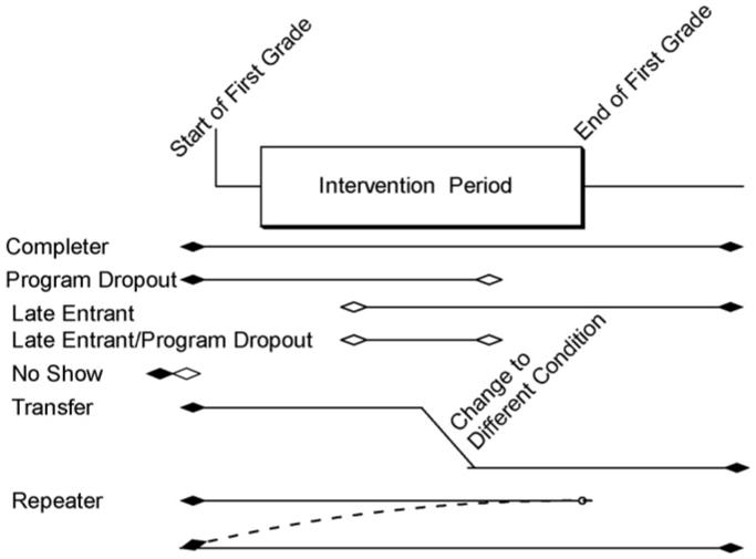
Classification of individuals based on entrances and exits.

Table 2.

Classification of individuals based on entrances and exits for the first and third Baltimore Prevention Program trials

	Type	1st Generation BPP Trial (intervention through 1st and 2nd Grades)	3rd Generation BPP Whole Day (WD) Trial (intervention through 1st Grade)
1	Completer	Any child who began attending first grade in one intervention condition and remained in one of the study classrooms to the end of second grade.	Same definition through 1st Grade.
2	Program dropout	Any child who began first grade in one intervention condition, was exposed to a portion of the intervention and moved outside the study’s classrooms prior to the end of the second year.	Same definition through 1st Grade.
3	Late entrant	Any child who transferred into one of the study’s first grade classrooms after intervention began and remained in one of the study classrooms through the end of the second year.	Same definition through 1st Grade.
4	Late entrant/program dropout	A child who entered one of the study classrooms after the intervention began and moved outside the study’s classrooms prior to the end of the second year.	Same definition through 1st Grade.
5	No show	No data available.	Any child who was registered to attend a study school during the summer before first grade, was assigned to a first-grade classroom but never attended the school.

The First and Third BPP trials point out the two alternative definitions of which individuals to include in ITT analyses. In either case, our first priority with these denominator definitions is to make sure that there is equivalence across intervention conditions, in the face of potential treatment dropout as well as later in terms of study dropout (Kleinman et al., 1998). Successful random assignment of groups generally allows for balance across baseline covariates for those who are present prior to randomization (when significance testing accounts for intraclass correlation and group random assignment). However, as we will see below, it is possible with some designs for late entrants to be placed differentially in the intervention conditions, so their automatic inclusion in the denominator may lead to nonequivalence. The second priority is to include the largest number of subjects with baseline data in these definitions, since this increases power in discriminating both main effects and interactions involving baseline (Brown and Liao, 1999; Roy et al., 2007). The two alternative denominator definitions are presented in Table 3.

Table 3.

Comparison of two definitions of individual level denominators for ITT analyses in multilevel randomized field trials

Equivalent intervention arms	Include in denominator	Strength	Weakness	When to use
Prior to start of intervention period	All subjects except those who are late entrants	Protects against subjects withdrawing differentially after being exposed to intervention	Limits sample size to those who enter at beginning of intervention period	When we do nothing in the design to assure late entrants will not be selected differently across intervention conditions
All subjects throughout intervention period	All subjects	Larger sample size; generalizes to all subjects, including those who after intervention period begins	Impact likely attenuated by less intervention exposure of late entrants	When there is assurance that late entrants are not being selected differently across intervention conditions

The first definition consists only of those individuals present at the beginning of the intervention period, in all those groups where random assignment to intervention is to take place. This automatically protects against late entrants being differentially placed in intervention or control conditions. Indeed, the data from the First Generation BPP trial suggest that principals were more likely to place late entrants in GBG classrooms, possibly because they felt that the late entrants would be more likely to be aggressive, disruptive and thereby would receive more intervention. To protect against this, in evaluating the Good Behavior Game in the First Generation BPP trial, the appropriate individual level denominator consists of all first graders who were assigned to any of the GBG classrooms and all controls, excluding late entrants and program dropouts/late entrants. Balance across intervention conditions is provided by randomization at the classroom level, as demonstrated by nonsignificant differences in baseline characteristics by intervention condition in multilevel models that account for the group level of randomization (i.e., Section 2.4 of Kellam et al., 2008). Because this denominator is formed from the population that is present before the intervention occurs, it is not subject to treatment dropout. Thus this denominator involving all those present at baseline is always appropriate for any trial in ITT analyses. In the First Generation BPP trial, this definition is used.

The second definition of the individual level denominator, which is appropriate for some but not all trials, would include those entering the study during the intervention period. There are some RFT designs that do provide good assurance of no differential treatment drop-in, and therefore in these cases it would be appropriate to include late entrants and program dropouts/late entrants as well. We have already pointed out that in school-based designs late entrants are highly unlikely to be informatively choosing which school to attend. Thus it is possible to exclude or include late entrants in school-based trials and still maintain balance.

It may be appropriate to include late entrants in some classroom and other designs as well. The Third Generation BPP trial is a good example of this. Unlike the first generation trial, this trial randomly allocates every child entering first grade in the 12 study schools to a classroom, using pre-sealed envelopes. A separate computer generated randomization is used to assign classrooms and their teacher to intervention condition. Our research protocol had us continue to assign children randomly to classrooms, even if they were late entrants, to ensure that the classes were balanced across the entire study. The only departure from this rule occurred if the classes within a school became too imbalanced due to differential rates of program dropout. Thus late entrant students were also balanced across intervention conditions, and they should therefore be included in the denominator, with a potential increase in statistical power. Comparing this case to the First BPP trial that was begun in 1985, in the earlier trial, we provided no protocol for incoming students, and therefore they were assigned by the principal in ways that may have used knowledge of which intervention was taking place in which classroom.

For the other RFTs we have provided descriptions of denominators for ITT analyses in Table 1, Column 3. In the Rochester Resilience Program (RRP) (Row 1), which used individual level assignment of at-risk children blocked within schools, the ITT denominators consist of all children who were eligible, consented, and randomized, just as in a standard P-RCT.

In the Georgia Gatekeeper Trial (GA Gatekeeper) (row 4 in Table 1), the most appropriate denominator to use consists of those present at the beginning of the school year. As with all school-based trials, the Georgia Gatekeeper research team had no influence over which students moved to different schools within the school year, and all these youth were exposed to that school’s intervention. Also, all schools in this study received the same gatekeeper training, with only the timing being randomly determined; therefore it was unlikely that any informative mobility occurred with regard to the intervention status. The denominators we used in our analyses were based on beginning year cross tabulations of numbers of subjects by gender, race/ethnicity, grade, and school because they were reported by the schools. Slightly more accurate denominators would have been based on population counts that had been averaged over the entire year, but such data were not available.

In the Adolescent Substance Abuse Prevention Study (ASAPS) (row 5 in Table 1), the intervention was held in both seventh grade (middle school) and ninth grade during high school. In this design all middle schools that fed into the same high school received the same intervention as did the high school. High schools were also geographically separated from one another so there was relatively little chance that those who migrated out of one study school would enter another study school. Because this study randomized schools, and intervention status likely had no influence on entrance or exit from the schools, the choice of including or excluding late entrants would likely not affect the equivalency by intervention condition. The decision of who to include in ITT analyses was therefore made based on criteria other than balance. First, because of the importance of the seventh grade component to this intervention, the investigators’ primary interest was in examining impact on the population who were in study schools in seventh grade, not those who transferred in to schools by ninth grade. Secondly, because there was strong interest in understanding whether the intervention effect was different among those youth who were initially using or at high risk for using substances compared to those who were not, a decision was made to limit ITT analyses further to all those who had baseline data at the beginning of seventh grade. These priorities had the effect of excluding those late entrants who came in to the school after the start of the first intervention in seventh grade.

Finally, in the California multidimensional treatment foster care (MTFC) trial (row 6 in Table 1), two different methods are being tested for implementing MTFC in California counties. Inclusion/exclusion criteria have been specified for determining which counties are to be randomized these two conditions. The primary outcomes relate to the time it takes for a county to begin placing families in MTFC. As for units lower in level than the county, system leaders, agency directors, and practitioners are assessed both prior to and through the intervention period. Changes in their responses on climate and attitudes are considered outcomes, and the composite is evaluated formally by intervention condition. These leaders, directors, and practioners are sampled systematically across the two conditions and across time. For ITT analyses, the late entrant individuals are included because of the high turnover in these positions over time, and these new individuals would need to be included to fully assess climate and culture. We also consider staff turnover as an outcome in its own right. Units in two other levels lower than county depend heavily on the success of program implementation, and are therefore evaluated in post-intervention analyses rather than ITT analyses. These include the selection of mental health agencies within counties to be trained to deliver MTFC, and the recruitment of new foster parents who are willing to be part of a treatment team to deliver a set of integrated services to youngsters with severe emotional and behavioral problems. Both of these selections occur as part of the implementation process. Because the recruitment of foster parents is different from that involving other types of foster care, and the primary focus is on the county and the agency, no formal ITT analyses of impact are likely to be done at the level of the foster care families; instead ITT analyses are being done at the level of the county and agency.

2.2.2. Defining individual level intervention condition and exposure in multilevel RFTs

In the previous section, we have specified ways to determine whether late entrant individuals should be included in the denominator of an ITT analysis. This section presents rules for assigning the intervention condition to subjects whose intervention exposure changes because of mobility. Along this second dimension of exposure to the intervention condition, each subject can be assessed on whether he or she received more or less intervention than planned, and whether the assignment of the child to an intervention adhered to the research protocol or not. These classifications are provided in Table 4, and we apply them to the Third Generation Baltimore Prevention Program Trial involving the Whole Day intervention. Children could have been exposed to less than the intended one year of intervention—which we have labeled intervention transfers, or more than the intended school year—which occurs if someone is a repeater, since sequential cohorts of children were given the same intervention in this study. In addition, we assessed whether the youth attended the intervention condition that was intended by the group-based randomization schedule or whether he or she received another condition, in which case we would identify this as a research protocol violation. Also, we identified the intervention of first exposure based on the first contact that child had with either of the intervention conditions.

Table 4.

Characteristics based on intervention exposure with examples from the third Baltimore Prevention Program whole day (WD) trial

	Type	Description	Research protocol violation
A	Intervention transfer	Any child who began first grade in one classroom and then moved or was otherwise assigned to another classroom. With a different intervention. It may be advantageous for some analyses to calculate the timing and length of exposure to each of the interventions.	No protocol violation if done for school administrative purposes.
B.	Repeater	Any child who began first grade in one of the study classrooms, then was held back or otherwise repeated first grade in one of the study schools—and therefore repeated exposure to the intervention. For repeaters, the intervention should be the same as in the previous year.	No protocol violation if done administratively by the school and the intervention condition is maintained.
C.	Intended intervention assignment	The classroom assignment designed by the research staff. In this WD trial, all classroom assignments were to be based on a sealed, sequential list of classroom assignments within school as children entered first grade throughout the year.	Any child who is placed in or removed from an intervention condition that was not intended by the planned research design results in an assignment protocol violation, and these should be reported as part of the CONSORT report.
D.	Intervention of first exposure	This is the intervention condition to which the child is initially exposed upon entry to the study.

For ITT analyses, individual intervention assignment should be based on the intended assignment if the assignment of individuals is to the intervention or to a group that itself is randomly assigned to an intervention. Furthermore, no one should be excluded because they received less than, or greater than the intended amount of intervention. Therefore, in the Rochester Resilience Project, the designated random assignment of the intervention condition should be used even if this particular intervention is not delivered to that individual. For the two BPP trials, the intended intervention assignment is determined by the assigned first-grade classroom. If there is no formal assignment of individuals, the intervention of first exposure is used to define each individual’s intervention condition. Using this rule, repeaters should be classified by their first intervention condition, even if they happen to be re-randomized to an intervention in the following cohort. Another example of this first exposure rule occurs in the Adolescent Substance Abuse Prevention Study, a school-based intervention trial. Here the school first attended during seventh grade determines the intervention status, regardless of their intervention status during the ninth grade intervention. These definitions naturally avoid any possibilities that a good or bad intervention experience could affect how a subject’s intervention classification. This rule also corresponds closely to that used in P-RCTs.

The Georgia Gatekeeper trial, which randomizes when schools get trained (Brown et al., 2006), deliberately changes intervention status at random times. As a consequence, we have had to adapt our ITT rule for classifying individual level intervention assignment accordingly. In this trial, the goal is to evaluate how many youths are referred for suicidality from schools where training has or has not occurred, over the three years when the trial took place. Schools were randomly assigned to when the training of the staff would occur. Because of confidentiality issues, we did not obtain any individual level identifiers; instead the referred youth were only identified by date of referral, school, grade, gender, and race/ethnicity. As we described above, the school district supplied overall numbers of youth at the beginning of each of the three years in each school’s grade, gender, and race/ethnicity cross-classification, and these were used to compute rates of referral for each, school, grade, gender, and race/ethnicity, and intervention status determined by the times that training of each school began. Without the ability to identify referred youth, we do not know if a referred youth had recently been in another school, so from a practical standpoint, all referrals for suicidality were assigned to the school where that referral took place, and assigned to condition depending on whether that school had already been trained or not as of that date. It is possible, although unlikely, that a referred youth in one school had recently moved from a school with a different training condition, and that a staff member from the former school had belatedly referred this student. If we had complete data, we would prefer to conduct ITT analyses by classifying where each child was at the beginning of each new training period, rather than the school attended at the time of referral. Thus our assignment of intervention status by current school, rather than initial school, for any mobile youth who was referred for suicidality, goes against our rule for classifying subjects to intervention condition in ITT analyses. In this way it is not a perfect ITT analysis, and this should be stated in publications.

In the Georgia Gatekeeper trial, we also followed up a stratified random sample of school staff from these same schools in Georgia in order to assess how gatekeeper training affected their knowledge, attitudes, and behaviors related to referring suicidal youth (Wyman et al., in press). Some of the staff, just like the students, moved during the study from a school in one training arm to a school in the other training condition. For ITT analyses, we coded these mobile school staff as belonging to the school where they first worked, a definition that is completely defensible but ignores whether or not that particular staff member was in fact trained (approximately three-quarters of staff per school were trained). Results from these ITT analyses on changes in assessments of staff could then be compared to results from “as-treated” analyses. In these “as-treated” analyses, the intervention condition for staff was the actual training condition they received, and in multilevel analyses their assignment to school was based on the most recent school where they were employed, not the first one. As expected, the ITT impact analyses showed somewhat smaller training effects than those in the “as-treated” analyses.

2.2.3. Practical issues in determining individual level denominator

From a practical point of view, the exact definition of the denominator will need to be based on the available data; rarely will complete tracking data be available to identify each child’s full entrance and exit history. Besides the cost involved in tracking individuals, the cost of obtaining consent can lead to practical choices affecting the denominator. It is often impractical to continue obtaining parental informed consent and a minor’s assent to participate in the study once the intervention has begun, so late entrants may need to be excluded based on this lack of informed consent. In the First BPP trial, we selected as our denominator those on the up-to-date class lists at the time of the baseline teacher ratings, 8-10 weeks into first grade just prior to the start of the intervention. This criterion thus excluded those who came in after the intervention period began—the late entrants—but potentially could also have included a few individuals who entered after the baseline data were collected but before the intervention began. This definition of the denominator based on class lists at baseline also had the practical advantage of minimizing the amount of missing data at baseline.

In the Third Generation BPP trial, it is illustrative to follow how we handled three students. Student 1 was enrolled in one of the twelve schools at the beginning of the school year and randomized to a classroom that would later receive the Whole Day (WD) intervention. The student transferred to another school before the intervention began, equivalent to a “no-show.” We thus excluded this individual from analyses. Student 2 enrolled into a study school in the final month of the school year and was randomly assigned to a treatment condition; however, she was exposed to that treatment condition for only three weeks. Because this trial continued to randomly assign children to classrooms, we chose to include this late entrant in our ITT analyses despite the limited intervention exposure. Finally, also in the final month of the school year, Student 3 was administratively moved from a standard setting classroom into the WD classroom in violation of random assignment, but in keeping with the school’s procedures for addressing student behavioral issues. This would be a research protocol violation even though it follows school protocol. We would include this subject and continue ITT analyses that assign this individual to control, the first intervention received.

2.2.4. Handling missing data in ITT analyses in multilevel RFTs

Missing data can arise at any level of analysis, but it typically occurs at the individual level where the different entrances and exits, missed assessments in a longitudinal design, and refusals to answer certain questions create varying patterns of incomplete data. One simple method that has been used to handle incomplete data is to remove any cases with missing data on any variable used in an analysis; however, this method uses post-intervention information to define who should be in the analysis, which is inappropriate for ITT analyses. It can also produce distorted inferences if subjects are attrited differentially based on the intervention condition.

Two acceptable methods of handling missing data for ITT analyses are the full information maximum likelihood method (FIML); (Little and Rubin, 1987), and multiple imputation (Rubin, 1987, 1996; Schafer, 1997; Schafer and Graham, 2002). FIML estimates are computed by maximizing the likelihood based on the variables observed for each case, assuming that the data are missing at random (Rubin, 1976), sometimes averaging over covariates that predict missingness (Baker et al., 2006). Multiple imputation forms a set of complete datasets based on an imputation model, then uses an analytic model to assess intervention effects on each of the completed datasets. The imputation model used to replace the missing data should always be at least as complex as the analytic model used to examine intervention impact (Collins et al., 2001; Graham et al., 2006, 2007; Schafer, 1997, 1999; Schafer and Graham, 2002).

For both the FIML and multiple imputation methods, the computations are based on an assumption of missing at random (Rubin, 1976; extensions for each method are, however, possible but less often used). This technical condition of missing at random holds either when the data are missing as if someone wiped off some data without regard to any of the values—or more generally when missingness of a datum is allowed to depend on other variables that are observed, but not allowed to depend on any of the unobserved variables.

An illustrative example of this more general case of missing at random is a two-stage follow-up study. Often used in psychiatric epidemiologic studies to provide cost-effective prevalence estimates, this type of planned missingness design is also appropriate for evaluating intervention impact—as well as variation in impact—on a diagnostic measure. Such a two-stage design was used in the First Generation BPP trial, and here we demonstrate the use of FIML to assess two aspects of the GBG impact on DSM diagnosis of Conduct Disorder (CD) by sixth grade using the Diagnostic Interview Schedule for Children (DISC 2.3-C; Fisher et al., 1992). The entire sample of first graders who remained in Baltimore City schools by sixth grade was assessed with an inexpensive screening instrument that contained a short list of CD items. All of those children who said yes to three or more questions were considered screen positive. All of these screen positives, plus a random sample of screen negative children irrespective of intervention condition, were then given a full DISC assessment of CD. The number of screen negative children that were given this second level assessment was somewhat less than the number of screen positive children. Overall, well over half of children in the sample were missing on the more expensive DISC assessment, yet accurate estimates of DISC-CD diagnoses can still be made because the reasons for missingness are completely known. By dealing with these data that are missing by design, the population proportions of both the GBG and control exposed subjects meeting diagnostic criteria could be computed using FIML methods. What follows is a standard FIML analysis that compares the overall rates of DISC CD diagnoses for the GBG and internal GBG controls for males in the first cohort.

Table 5 collapses the results of a four-way tabulation of individuals by intervention condition, screen status, status on a DISC-CD diagnosis, and whether or not the youth was selected to receive the DISC. The whole numbers in the table refer to the numbers of subjects observed in this cross classification. Thus in the first row of data, one GBG exposed male received a positive DISC diagnosis after being screened positive, and six received a negative DISC diagnosis after being screened positive. Also on this same row, there were no GBG screened positive males who were not assessed on the DISC. This is because all those who were screened positive are assessed on the DISC so there are no missing DISC data for these individuals.

Table 5.

Estimates of screening status by DISC diagnosis of sixth grade males exposed to good behavior game or internal GBG control conditions

	Screen\DISC status	Received DISC assessment		Did not receive DISC assessment
		DISC-CD positive	DISC-CD negative	DISC-CD positive	DISC-CD negative
GBG (N=53, 7 screened positive, 46 screened negative, 44 not assessed on DISC	Positive screen	1	6	0	0
	Negative screen	0	2	44×p0	44×(1-p0)
Internal GBG control (N=30, 11 screened positive, 19 screened negative, 18 not assessed)	Positive	5	6	0	0
	Negative	0	1	18×p0	18×(1-p0)

Note: DISC = diagnostic interview schedule for children.

Note that the first two columns of cell counts correspond to the numbers of males who received both the screen and the DISC, while the remaining two columns correspond to both observed and estimated cell counts for those who were not chosen to receive the DISC. There were 44 (=53-1-6-0-2) GBG males who were screened negative who did not receive the DISC, and similarly there were 18 (=30-5-6-0-1) internal GBG controls who were both screened negative and not selected for the DISC. We expect the same proportion of these non-assessed, screened negative males (p₀) to be DISC-CD positive for GBG and internal GBG control males, since the assessment was blind to intervention condition. Our best estimate of p₀ based on both cohorts was 2/27 = 0.069; this is the observed proportion of screened positive males who were found to be DISC positive. This maximum likelihood value has been used in Table 5 to obtain the expected number of DISC-CD positive males in each condition by collapsing across the two tables where the DISC was taken and where it was not taken. Standard errors (in parentheses in the last column) as well as the correlation among these estimates (not shown) are computed based on the Delta method.

A formal test of equivalence in CD prevalence by intervention condition using these data above was rejected. There were significantly lower odds for GBG exposed males compared to the internal GBG control males (OR = 0.31, 95% CI = 0.10, 0.95). Thus overall reduction in CD in the GBG condition is evident by grade six, preceding the result we report on reduction in adult antisocial personality disorder diagnoses (ASPD) among the first grade aggressive, disruptive males (Petras et al., 2008). This makes sense because conduct disorder during adolescence is a requirement for an adult ASPD diagnosis. These findings were also similar to that for adult diagnostic outcomes (Kellam et al., 2008), where GBG exposed children in the first cohort had substantially reduced drug abuse/dependence disorder diagnoses. These findings on CD were not replicated in the second cohort where less impact was generally seen.

Multiple imputation (MI) can also be used to handle missing data by replacing missing observations based on an imputation model with multiple versions of a complete dataset. These complete datasets are then analyzed using standard statistical methods, and inferences on such statistics as the odds ratio for GBG versus internal GBG control DISC diagnoses, are made by accounting for two sources of variation: the average standard errors of the odds ratios (within variation) and the variation in these odds ratios across the multiple imputations standard errors (between variation). Confidence intervals can also be formed according to Rubin (1987, 1996) and Schafer (1997, 1999).MI has some advantages over FIML since it can use this additional information to impute values from a large number of observed extra variables that never appear in the final analysis. FIML can also be used with a modest number of extra variables, collapsing over those not used in the final model as we did in Table 6.

Table 6.

FIML estimates of the relation between intervention and DISC conduct disorder diagnoses in sixth grade

Intervention	Estimated numbers with DISC-CD positive	Proportion DISC-CD positive (standard error)
GBG (N=53)	1+0+0+44×p0 = 4.03	0.076 (=4.03/53) (0.032)
Internal GBG Control (N=30)	5+0+0+18×p0 = 6.24	0.208 (=6.24/30) (0.170)

As an example of how MI can be used in ITT analyses, we refer back to the GBG impact analyses of on adult drug dependence/abuse diagnoses, taking into account the baseline levels of aggressive, disruptive behavior in first grade on this outcome (Kellam et al., 2008). There were some missing data on both the first grade aggressive, disruptive behavior measure as well as the distal outcome; intervention status was available for everyone. FIML analyses of intervention impact in this particular case would typically ignore any missing data on either baseline or outcome (Brown, 1993b). However, the imputation model can use additional information on other variables measured across the study to help assess intervention impact. In our analyses reported in Kellam et al. (2008), we included self-report measures of depressive symptoms in the imputation model and concluded that the effect was stronger using multiple imputation compared to the traditional FIML model.

We also note that a small number of imputations, say three to five, can often provide enough complete datasets to provide good quality inferences about intervention impact (Rubin, 1987). Recently, there have been recommendations for using an order of magnitude more imputations in complex, large datasets with many variables used for imputation (Graham et al., 2007). The larger number of imputations is of direct value when making confidence intervals for examining variation in impact as well.

As a final point of comparison, some individuals may be measured at baseline but may be completely lost to follow-up and have no measures taken beyond baseline. With FIML, such individuals contribute nothing to the likelihood and therefore are effectively excluded from analyses. With MI, these individuals contribute a small amount of information based on their baseline data; their effects on the final inferences are generally small.

2.3. Modeling strategies to examine who benefits or is harmed in ITT analyses

With ITT procedures now defined, we can proceed to discuss analytic strategies for examining impact in such trials. Such methods have evolved from simple comparisons of proportions, as with the CD analyses above, to adjusted means in analysis of covariance, to methods that incorporate nonlinear modeling (Brown, 1993b; Hastie and Tibshirani, 1990), growth modeling (Muthén, 1997, 2003, 2004; Muthén and Curran, 1997; Muthén and Shedden, 1999; Muthén et al., 2002) and multilevel modeling (Gibbons et al., 1988; Goldstein, 2003; Hedeker and Gibbons, 1994; Raudenbush, 1997; Raudenbush and Bryk, 2002; Raudenbush and Liu, 2000). Since a recent listing of such methods and their use in the BPP First generation trial is available elsewhere (Brown et al., 2008), we highlight only a few novel applications for RFTs in this paper. Our presentation begins with examining impact for a single follow-up time and initially treats the multiple levels in the design as nuisance factors. We describe the use of such methods on the First BPP trial where we examine impact on drug abuse/dependence disorder diagnoses (Kellam et al., 2008). The five other trials that were described earlier (Table 1) are used to illustrate how generalizable these methods are across a wide set of trials.

2.3.1. Theoretical models of variation in impact by baseline individual level risk characteristics

In P-RCTs the ITT analysis has traditionally been focused on examining main effects of the intervention (Friedman et al., 1998; see, however, Kraemer et al., 2002). Unless there is an a priori reason to hypothesize an intervention that interacts with baseline, the standard approach in P-RCTs has been to avoid testing for variation. This practice is conservative because one will never find any real or spurious variations in impact if one does not look for them. However, theoretically driven hypotheses can be examined through subgroup analyses in randomized trials. As an example, because of random assignment within a trial, control males and treated males should be equivalent at baseline, and their responses can be legitimately compared, as can those for females or other important subgroups.

One reason to search for variation is to personalize or tailor treatments to maximize impact among different subgroups (Rush et al., 2006), but this is a relatively new development. For most P-RCTs trials, the sample is deliberately chosen to be homogeneous, leading to limited variance in baseline characteristics, and consequently there is often little statistical power available to examine such interactions between baseline and intervention.

In RFTs, particularly those based on universal preventive interventions, there is almost always an a priori reason to examine interactions involving intervention and baseline level of risk. Many of these interventions are designed to modify one or more risk factor that is measured at baseline, and they are expected to be successful only through the modification of these risk factors. In addition, in group-based randomized trials, statistical power is much more heavily dependent on the number of groups rather than the individuals, so subgroup analyses and tests of interactions often do not suffer from poor statistical power the way they do in individually-based trials (Brown and Liao, 1999; Raudenbush and Liu, 2000).

We take as our first example the variation in impact we would expect to see in the First Generation BPP trial. The Good Behavior Game was designed to reduce aggressive, disruptive behavior. Because roughly half the children have minimal levels of aggressive, disruptive behavior on entry into first grade and also throughout childhood (Muthén et al., 2002), we predict that the GBG would have little or no effect on these children. For those with aggressive, disruptive behavior at baseline, many are expected to remain aggressive, disruptive in the absence of intervention (Moffitt, 1993; Moffitt and Caspi, 2001; Muthén et al., 2002), so for these high risk aggressive, disruptive children, we would predict that an effective intervention would show high impact. In terms of ITT analyses, these predictions can be tested by measuring the significance of interactions involving baseline aggressive, disruptive behavior and intervention.

There are other reasons for examining interactions between intervention condition and individual level baseline risk. For some individuals, an intervention may be harmful while it may be beneficial for others. In the Second Generation BPP trial, we tested a mathematics curriculum intervention for first graders. Overall it improved math achievement, but when we examined impact as a function of first grade baseline achievement, we found that it worked well for those with initially high achievement and was actually harmful for those who began with low levels of achievement (Ialongo et al., 1999). Videotapes of the intervention pointed to lower engagement with lower achieving children compared to high achieving children. Because of this disadvantage to less achieving youth, this intervention was not continued.

Variation by individual level risk is also important in selective and indicated interventions, especially as this can help determine an optimal cutoff in risk below which an intervention has limited effect (Tein et al., 2004). Alternatively, we may decide to modify an intervention so that its impact is improved over a wider range of risk.

While we have so far emphasized interactions involving risk measured at the individual level, such interactions can and often do extend to systems or contexts that are unique to the individual in a trial. That is, in a classroom-based trial, family environments of the subjects will have minimal overlap, but school and neighborhood environments may be partially or completely shared. Clearly, our ability to detect variation in impact across family, school, and neighborhood environments will depend on the degree of overlap. If there is no overlap, or minimal overlap across subjects, then a contextual level variable can be included in an analysis as an individual level variable. Thus in the First Generation BPP trial, family poverty status, measured by reduced or free lunch, acts as an individual level variable. This poverty index was found to contribute to the course of aggressive, disruptive behavior in the First Generation BPP trial, but the GBG succeeded equally with children in impoverished families and those with somewhat higher incomes (Kellam et al., 1998).

2.3.2. Theorizing variation in impact involving levels that are partially or completely shared

Randomized field trials with multilevel designs provide opportunities to examine variation not only by individual baseline characteristics, but by characteristics at higher levels, including those where the intervention assignment occurs and higher levels as well. Returning to the classroom-based First Generation BPP trial, we would expect impact to be low if the classroom began the year with an overall low average aggressive, disruptive score. At the other end, we would expect the impact to be potentially high in classrooms that started with high classroom average levels of aggressive, disruptive behavior. Only in these classrooms where a teacher has difficulty managing her class would there be a strong potential for the intervention to make an impact. All students in the classroom would share these teacher characteristics, although some children may be affected more than others.

Recall that in the First BPP trial children were balanced across classrooms within a school based on kindergarten performance. One might expect that this balanced assignment of children to classes within school that was carried out by this First BPP trial design (Kellam et al., 2008; Brown et al., 2006) would lead to nearly identical levels of classroom average aggressive, disruptive behavior within schools, and therefore we would have no ability to examine variation in impact by classroom average aggressive, disruptive behavior level once we blocked by school. However, this is not the case. After adjusting for school, we found significant classroom level variation in the average aggressive, disruptive score within classrooms early on in the school year before the intervention began, but there were no differences in this contextual level of aggressive, disruptive behavior by intervention condition (Kellam et al., 2008). In contrast to this varying level of classroom average aggressive, disruptive behavior, there was no significant classroom variation in classroom averages of achievement or family poverty; an additional source of classroom variation was occurring that affected the levels of child aggressive, disruptive behavior. Our working hypothesis that came out of these baseline multilevel analyses was that we did successfully balance children into classrooms on achievement and a poverty index, but the level of aggressive, disruptive behavior seen in classrooms was heavily influenced by the teacher’s ability to manage his or her classroom. About half the teachers were successful in managing classroom aggressive, disruptive behavior at baseline, while the other half were unsuccessful (Kellam et al., 1991, 1998). We would therefore predict that the GBG would have its highest effect in classrooms where the baseline level of aggressive, disruptive behavior was high, strongly suggesting that the teacher had limited ability to manage his or her classroom. The GBG’s effect would be low in well managed classrooms. Furthermore, we would predict that the GBG’s highest impact would be for the most aggressive, disruptive children in the most aggressive, disruptive classrooms, a three-way interaction. We tested for this three-way effect in previous analyses, and found this estimated effect was in the expected direction, but was non-significant (Kellam et al., 1998). Not surprisingly, the power for this three-level interaction was rather modest.

Intervention effects may vary as a function of neighborhood of residence and other contexts that are partly shared across these classrooms. While there have been several examinations of neighborhood effects on child development (Aber et al., 1997; Brooks-Gunn et al., 1993; Pickett and Pearl, 2001; Plybon and Kliewer, 2001), to date little attention has been placed on its moderating effect on a preventive intervention. The methodology is available, however, to address such questions.

Interactions between baseline and intervention conditions have been hypothesized for the other trials that we have included in Table 1 as well. For the Rochester Resilience Project (Row 1), we hypothesized that the intervention effect would vary as a function of classroom context, with higher impact when the proportion of children in the classroom were maladapting. In the Third Generation BPP trial (Row 3), we elaborated on the model developed for the First Generation trial. The prediction is that intervention impact would be expected to be greatest on children who were aggressive, disruptive or poor learners at baseline in classrooms where the teacher had low management skills and had limited effectiveness in teaching reading. In the Georgia Gatekeeper Project (row 4), we hypothesized that QPR training would be more effective in referring suicidal youth in middle school compared to high school, both because of elevated suicidality in middle school but also closer contact with school staff for these younger children. In the ASAPS school-based trial to prevent drug use (row 5), we anticipated variation in impact by individual level of risk regarding attitudes and usage of drugs as well as low bonding to school in seventh grade. We also predicted that in schools where the school-level norms regarding use of drugs were high at baseline, the intervention effect would be larger since that was one of the targets of the intervention. Finally, in the California MTFC trial (row 6), we anticipate there may be differences in impact for rural versus urban counties, as well as those counties that have a history of interagency collaboration.

We have specified important baseline by intervention interactions in each of these trials based on theory. In the next section we examine how inferences about overall intervention impact as well as variation in impact can be drawn from analytic models that may be imperfectly specified.

2.4. Causal inferences regarding overall impact and variation in impact for RFTs

All ITT analyses of intervention impact involve a comparison of responses among those assigned to the intervention compared to those assigned to another (control) condition. This comparison may be simple, for example, a difference in observed means for each group. The comparison could also involve complex, sophisticated models with random effects, covariates, and interaction terms that are linearly or nonparametrically related to outcomes, whose outcomes themselves may have normal, binomial, count, or time to event distributions (Brown et al., 2007d; Kellam et al., 2008). Statistical inferences derived from these models are then used to infer causal effects due to the intervention. Random assignment helps considerably in strengthening these causal inferences about the intervention, but most trials use random assignment at only one level. It is not immediately clear whether statistical inferences about parameters measuring variation in impact across different levels of a trial have causal interpretations, nor is it clear whether our causal inferences remain valid if we fail to specify all the appropriate covariates in our model. Such fundamental questions of causal inference have been partially answered through advances in causal modeling. These advances include the Neyman, Rubin, Holland (NRH) approach involving potential outcomes or counterfactuals of the primary outcome (Holland, 1986; Neyman, 1923; Rubin, 1974, 1978) and a principal stratification approach involving intermediary outcomes, such as participation or adherence as well (Angrist et al., 1996; Frangakis and Rubin, 1999, 2002; Jo, 2002; Jo and Muthén, 2001). In this paper involving ITT analyses, the NRH approach allows us to obtain some general rules on when the statistical models provide valid causal inferences. For post-assignment analyses that we have not included in this ITT paper, we would need to rely on principal stratification as well.

2.5. Assignment adjusted analyses to improve inferences of intervention impact

Making correct inferences about intervention impact requires us to include in our model the right covariate terms involving the intervention. Thus if the intervention effect varies by baseline levels of risk, the model should include an intervention by baseline covariate along with intervention itself. Without these terms in the model, we cannot expect to make correct inferences about the intervention’s full impact. A more troubling issue, however, is whether our conclusions about an intervention’s variation in impact depend on whether we build a model that includes all important covariates, even ones at the individual level that do not include intervention condition. If our inferences about intervention impact did require us to include all important individual level covariates in our analysis, then our inferences from a best-fitting model could be suspect. This section describes a general procedure called assignment adjusted analysis that automatically protects our inferences in RFTs against some missing covariates.

For trials that randomize at the individual level, it is well known that randomization protects inferences of overall intervention impact in case we have an incomplete model. We may be missing an important individual level covariate, but randomization provides balance across this missing covariate. The situation is not exactly the same in trials that are randomized at the group rather than individual level, but there is a relatively simple method that can provide this additional stability in these estimates of intervention impact even if we ignore or do not have available some important predictors.

In this section we provide a method that produces accurate estimates of intervention impact even if the underlying model is not specified completely. To study the properties of these estimates, we distinguish between a NRH causal model involving possible outcomes that describes how each subject’s outcome, if assigned to the control condition, would depend on individual level and higher level covariates (Brown et al., 2007b). The causal model would further specify how each individual’s outcome, if assigned to the active intervention condition, would depend on additional individual level and higher level covariates as well. The causal effect for each individual is then defined as the difference in the outcome under active intervention and control conditions. These causal effects contain the true parameters that represent intervention impact. If the causal effect is just a simple constant difference between intervention and control, then the only intervention effect is a main effect. If the causal effects vary as a function of a covariate, then the intervention effect interacts with that covariate.

Because we can never know the true causal model for the data, we can only evaluate intervention impact on a hypothesized multilevel model that specifies how each subject’s outcome depends on their intervention status, covariates, and interactions, as well as error terms accounting for individual and shared variances. There are three important possibilities to study; this hypothesized model, evaluated for those who are included in the study and under the random assignment mechanisms, may be: (1) exactly correct; (2) it may be overly inclusive by containing more covariates than the true model; or (3) it may be under inclusive of the true covariates or interactions affecting outcomes. Theoretical developments have shown that under mild assumptions about the models and the ways that individuals and higher level units are selected and assigned to the intervention conditions, hypothesized models that are exactly correct or over specified will yield unbiased estimates of all the intervention effects. If the hypothesized model is underspecified, inferences about intervention effect can be erroneous. Some estimates of intervention effect perform well when subjects are weighted inversely in proportion to the probability of intervention assignment (Rosenbaum, 1987), but this is not necessarily the best approach when examining variation in impact. It is always possible, however, to add some simple covariates in an underspecified model and thereby produce an asymptotically unbiased estimation of intervention impact, even when some of the covariate predictors are not in the hypothesized model. We call this procedure assignment adjusted analyses (Brown et al., 2007b).

Specifically, we first calculate the proportion of groups in each block that are randomly chosen to receive the intervention. If this block level “propensity” measure is constant, that is, the proportion of groups in each block receiving the intervention is the same, then the model is robust against under specifying the covariates. That is, even when important covariates at any level that do not involve the intervention condition are not included in the analysis, the overall impact estimates remain unbiased. Only in the case where these propensities are not constant is there any benefit to making an adjustment. The adjustment is straightforward (Brown et al., 2007b): simply add new covariates to the model corresponding to the propensity score variable itself and the product of any covariate that interacts with intervention assignment. Thus if only a main effect of intervention is being examined (Tx = 1 if active intervention, Tx = 0 for control) for its effect on a continuous outcome, one would include in a linear mixed model (LMM) analysis a new covariate π, corresponding to the proportion of the groups assigned to active intervention within each block. For example, in a classroom-based randomized trial, if two of the three classes in a school (that is, the blocking factor) were assigned to active intervention, then π = 2/3 for every individual subject in this school. This covariate π is a true propensity score, but unlike traditional propensity score analyses (Rosenbaum, 1987), it need not be estimated from a model but rather it is obtained from the numbers of units that are actually assigned to the active intervention within each block.

We now describe the assignment adjusted model that is necessary when more complex baseline by intervention interactions are added to the model. If a main effect of intervention Tx is included as well as an interaction of this intervention condition times a covariate X, Tx × X, then we would add into our analysis both the propensity score covariate π and the interaction term π × X. Two examples from the First Generation BPP trial are presented below followed by a more general rule for incorporating model robustness. In this RFT trial, level one corresponds to individuals, level two corresponds to classrooms, and level three corresponds to schools (which were further nested into geographic areas of the city). Furthermore, the two outcomes we examine are binary, so generalized linear mixed models, which is logistic regression with random effects, is used instead of LMM.

First, we present the impact of the Good Behavior Game on lifetime drug abuse/dependence disorders by age 19-21 as described in Kellam et al. (2008). In the generalized linear mixed effects model analysis presented in Table 7 for males, which adjusts for classroom variation and baseline aggressive, disruptive behavior ratings from first-grade teachers, the reduction in lifetime drug abuse/dependence disorders for GBG compared with internal GBG controls was large and significant, with a log odds ratio (OR) of 0.999 (p = 0.035) as shown in the third row of Table 7. This magnitude corresponds to an approximately 2.7 times greater risk of drug abuse/dependence disorders in the internal GBG controls compared with the GBG. In contrast to this significant difference between the GBG and internal GBG controls, there was no indication of differences in rates of disorders among the three control groups (internal GBG, internal ML, and external controls); see contrasts in rows 4 and 5 of this table. In this best fit model, there were no significant interactions between intervention and baseline aggressive, disruptive behavior. To further ensure the unbiasedness of the estimated treatment effect, we added assignment adjustment by including the probability of GBG assignment (π) as a main effect. For all individuals in the same school, the value of this covariate π was the same, simply the proportion of the classes that were assigned to the GBG. These propensities varied from 1/2 in schools that had two classrooms to 2/3 for schools that had three classrooms with two assigned to the intervention. In the assignment adjusted GLMM analysis summarized in Table 8, we have carried out the same analysis by now adding the propensity covariate to the analysis (row 3). The reduction in lifetime drug abuse/dependence disorders for the GBG compared with internal GBG controls was still large and significant (log OR of 1.068, p = 0.028 in row 4 of Table 8). Note that the intercept term (row 1) is the only one to change from Table 7; this is because the mean of π is far from zero. Note also that the two contrasts in rows 5 and 6 lose precision; this is because π is strongly correlated with these two dummy variables (π = 0 for all children in external control and ML schools). These differences do not change the conclusion that the GBG was effective.

Table 7.

Generalized linear mixed model (GLMM) results for lifetime drug abuse/dependence disorders among males with no assignment adjustment (N=269 students, 31 classrooms)

	Coefficient (S.E.)	d.f.	t-value	p-value
Fixed effects
Intercept	-1.442 (0.396)	237	-3.642	<0.001
Baseline aggressive, disruptive behavior	1.200 (0.299)	237	4.019	<0.001
GBG vs. internal GBG control (Tx1)	-0.999 (0.450)	27	-2.221	0.035
External control vs. internal GBG control (Tx2)	-0.211 (0.403)	27	-0.525	0.604
Internal ML control vs. internal GBG control (Tx3)	-0.130 (0.448)	27	-0.291	0.773

	S.D.	p-valuea
Random effects
Classroom	0.003	0.488

^aFor testing zero variance.

Table 8.

Assignment adjusted GLMM model for lifetime drug abuse/dependence disorders among males (N=269 students, 31 classrooms)

Row		Coefficient (S.E.)	d.f.	t-value	p-value
Fixed effects
1	Intercept	-2.565 (1.627)	237	-1.576	0.116
2	Baseline aggressive, disruptive behavior	1.222 (0.302)	237	4.047	<0.001
3	Probability of GBG assignment (π)	1.941 (2.714)	26	0.715	0.481
4	GBG vs. internal GBG control (Tx1)	-1.068 (0.459)	26	-2.327	0.028
5	External control vs. internal GBG control (Tx2)	0.895 (1.604)	26	0.558	0.582
6	Internal ML control vs. internal GBG control (Tx3)	0.981 (1.622)	26	0.605	0.551

		S.D.	p-valuea
Random effects
7	Classroom	0.003	0.489

^aFor testing zero variance.

We now examine assignment adjusted analyses in the same trial but for an outcome that exhibits important variation in impact by baseline. For lifetime regular smoking of males, we reported a significant treatment impact as well as interaction with baseline aggressive, disruptive behavior (Kellam et al., 2008). We investigated how to perform assignment adjusted analyses for both of these intervention impact covariates. To determine those factors contributing to males smoking 10 or more cigarettes per day as young adults, we obtained a bestfitting GLMM model that included main effects for baseline aggressive, disruptive behavior plus interactive effects of baseline by intervention condition. A likelihood ratio test confirmed a highly significant effect of the GBG when compared with the internal GBG control (p = 0.003, with 2 d.f.). Overall, the GBG is associated with a reduction in the probability of males smoking 10 or more cigarettes per day, and the effect of the GBG was greater for boys with higher levels of aggressive, disruptive behavior in first grade compared with lower levels where the rates of regular smoking are similar (see row 6 of Table 9). This finding could also be verified by the assignment adjusted model, which is summarized in Table 10. We added two terms in the model. They are the probability of GBG assignment (row 3) and the interaction between the GBG assignment and the baseline aggressive, disruptive behavior rating (row 7). The overall significance of the GBG impact when tested with a likelihood ratio test had a p-value of less than 0.001 (on 2 d.f.). Compared to the unadjusted analysis, the treatment effect again showed very significant and higher benefit for the higher risk boys (row 8).

Table 9.

GLMM model for males smoking ≥10 cigarettes/day as young adults, no assignment adjustment (N=278 students)

Row		Coefficient (S.E.)	d.f.	t-value	p-value
Main effects
1	Intercept	-4.435 (1.239)	243	-3.579	<0.001
2	Baseline aggressive, disruptive behavior	3.306 (1.144)	243	2.889	0.004
3	GBG vs. internal GBG control (Tx1)	2.977 (1.441)	27	2.066	0.049
4	External control vs. internal GBG control (Tx2)	3.234 (1.345)	27	2.404	0.023
5	Internal ML control vs. internal GBG control (Tx3)	2.713 (1.376)	27	1.972	0.059
Interaction effects
6	Tx1 by baseline	-6.919 (2.094)	243	-3.304	0.001
7	Tx2 by baseline	-3.848 (1.273)	243	-3.022	0.003
8	Tx3 by baseline	-2.869 (1.313)	243	-2.184	0.030

	S.D.	p-valuea
Random effects
Classroom	1.048	0.196

^aFor testing zero variance.

Table 10.

Assignment adjusted GLMM for males smoking ≥10 cigarettes/day (N=278 students)

Row		Coefficient (S.E.)	d.f.	t-value	p-value
Main effects
1	Intercept	-2.023 (4.827)	242	-0.419	0.675
2	Baseline aggressive, disruptive behavior (X)	-3.491 (7.341)	242	-0.475	0.635
3	Probability of GBG assignment (π)	-5.337 (8.651)	26	-0.617	0.542
4	GBG vs. internal GBG control (Tx1)	3.578 (1.623)	26	2.204	0.037
5	External control vs. internal GBG control (Tx2)	0.807 (4.856)	26	0.166	0.869
6	Internal ML control vs. internal GBG control (Tx3)	0.273 (4.866)	26	0.056	0.955
Interaction effects
7	Probability of GBG assignment by baseline (π × X)	13.797 (14.482)	242	0.952	0.342
8	Tx1 by baseline	-8.452 (2.689)	242	-3.144	0.002
9	Tx2 by baseline	2.959 (7.362)	242	0.402	0.688
10	Tx3 by baseline	3.947 (7.370)	242	0.536	0.593

	S.D.	p-valuea
Random effects
Classroom	1.110	<0.001

^aFor testing zero variance.

2.6. Analytic considerations and strategies in examining variation in intervention impact

One of the major concerns voiced about the inclusion of interaction terms in the analysis of randomized trials is that these additional terms provide multiple opportunities to find significant intervention impact, thereby inflating the Type I error rate. Without taking some precautions, this inflation will be important because model complexity increases exponentially with additional covariates; these analytic complexities include the use of polynomial, nonlinear baseline terms and interactions or subgroup analyses. One systematic way to protect against inflating the alpha level is to: (1) start with the more complex models that include interactions and nonlinear covariate effects; (2) identify the best-fitting model by removing interactions and replacing nonlinear effects with linear effects; and (3) evaluate intervention impact in this best-fitting model. The key to limiting the alpha level is to ignore any examination of the coefficients of the intervention terms when deciding on the best-fitting model; only examine these intervention effects in a best-fitting model. This general approach was used in our ITT analyses of the GBG in the first BPP trial (Kellam et al., 2008).

Besides making assessments about whether to include nonlinear or linear effects or interactions in examining intervention impact, there are additional complexities that ITT analyses of variation in impact in RFTs often require: multiple levels of nesting in trials, random effects on the intercept and slopes, and non-normal models. Few analytical approaches can handle all these levels of complexity at the same time. Below we describe how a broad set of these models, as well as testing for variation in impact, can be handled with generalized additive mixed models, and then discuss analytical strategies that build on each component to form a completed set of analyses.

2.6.1. Generalized additive mixed effects model

GAMM is an extension of the Generalized Linear Mixed Effects Model, which itself is an extension of Generalized Linear Models (GLM; McCullagh and Nelder, 1989) as well as an extension of linear models such as regression, analysis of variance, and analysis of covariance. These linear models assume that the outcome distribution is continuous and nearly normally distributed. The GLM class of models contains all standard regression models with a normally distributed outcome, as well as logistic regression, Poisson regression, and log-linear models that include contingency table analyses (McCullagh and Nelder, 1989). GLMM adds random effects to all of these models so that multiple levels of clustering and longitudinal, repeated measures on the same subjects can be handled. Such models with both random and fixed effects are called mixed effects. Finally, GAMM allows the fixed effects in these mixed effects models to be related in nonlinear, smooth nonparametric relationships with the outcome measure. While GLMM does provide a form of nonlinear relationship to hold, this relationship is parametric and rigid in nature. GAMM’s added flexibility of using nonlinear, smooth relationships compared to linear relationships provides a valuable tool in assessing whether intervention impact is the same across all levels of a baseline characteristic or whether it varies by this characteristic.

2.6.1.1. Generalized additive model for binary outcomes

Diagnoses, as well as many other binary outcomes of interest, are poorly modeled using normal based models; the logistic model is traditional for binary outcomes. This logistic regression model posits a linear relationship between the logit of the conditional probability of the jth subject’s binary outcome Y_j being one (diagnosis) and covariates (X_j), e.g., baseline characteristics and intervention condition. The linear part of this model has the form of logit ((Pr(Y_j = 1/X_j)Σx_jβ_j), where the β_j are regression parameters.

From the linear logistic model and its regression estimates, one can interpret the intervention impact. In a model that includes intervention condition as an indicator of active intervention (one) compared to control (zero), the coefficient for intervention estimates the log odds of active intervention on outcome, adjusted for the other covariates. A value of zero implies that there is no intervention impact, and a negative value indicates that the outcome is less likely under active intervention compared to control. When the logistic model includes the intervention condition, a baseline covariate, and the product interaction of intervention by baseline, then the last coefficient can be used to measure the linear change in the log odds of intervention effect with a unit change in baseline.

The generalized additive model replaces Σx_jβ_j with Σf_j(x_j) where f_j is an unspecified smooth function; examples of these smooth nonparametric functions, which differ from linear fits, can be found in Fig. 2 discussed later. Under a conventional least square approach, f_j could be estimated by minimizing Σ(y_j - f_j(x_j))². In the generalized additive model approach, we maximize the log likelihood after adding a term that measures the “smoothness” of the function f_j to the target quantity being minimized. This means we do not just minimize the log likelihood but also take into account the smoothness of the regression curve. The function is often estimated in a flexible manner using cubic splines with variable nodes. This estimated function Σf̂_j(x_j) can reveal possible nonlinearities in the effect of the X_j. When one of the x_j corresponds to the product of intervention by baseline, this nonparametric function maps out how change in the log odds between intervention versus control changes as the baseline value is moved.

Fig. 2.

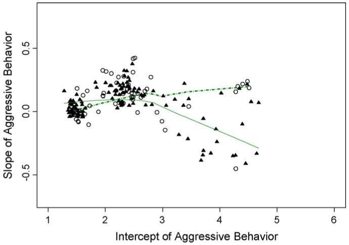
Nonlinear smooth fits of empirical Bayes slopes to intercepts for males in good behavior game (▲) and control (○) classes.

2.6.1.2. Generalized additive mixed model for binary outcomes

The generalized additive model can be extended to incorporate random effects for the mean/intercept. In the computation stage, the model fitting procedure is separated into two steps, the generalized additive modeling part and the linear mixed effects modeling part. These two steps are implemented iteratively to find the best solution. For computations, we have used R with the contributed package MGCV (R Project, 2007).

In RFTs, clustering at different levels can be incorporated in the model by adding random covariate effects (Gibbons and Hedeker, 1997; Gibbons et al., 1988; Hedeker and Gibbons, 1994). To test if inclusion of random effects helps with the model fitting, we can perform a likelihood ratio test. If the final candidate model is a generalized linear model, we can compare the fit using a generalized linear fixed-effects model with the same model that also includes random effects. Under the null distribution of no random effect, the test statistic follows a weighted Chi-square distribution; see Kellam et al. (2008) for examples of its use.

Once we have identified a best-fitting candidate model, we can add random effects from the next level (e.g. classroom, school, and geographical regions). If the variance of the classroom-level random effect is large, then we can investigate whether inclusion of fixed contextual variables provide additional explanatory value. Formal testing of whether the random effects are required in a model will depend on whether the best-fitting model is a generalized linear model, or a generalized additive model. For the former, we compared the fit using a generalized linear mixed-effects model (Breslow and Clayton, 1993; Wolfinger and O’Connell, 1993) while the latter, when there are significant nonlinear predictors, should be compared using a generalized additive mixed mode (Wang, 1998; Wood, 2004).

3. Analytical strategies for examining variation in intervention impact over time

In this section, we summarize how growth modeling can characterize the patterns of change in repeated measures over time due to an intervention compared to control. We consider many of these models as intent-to-treat analyses, and for some trials a growth model analysis may provide the primary analysis of impact, just as in P-RCT’s the primary analysis can be based on the rates of change in a repeated measure for intervention versus control (Muthén, 1997, 2003, 2004, in press; Muthén and Muthén, 1998-2007; Muthén et al., 2002). These growth models are quite flexible, incorporating linear or nonlinear growth patterns, interactions with baseline variables, intervention changes that affect the variance or covariance as well as the mean pattern of growth, and varying intervention impact across different patterns of growth, rather than an effect that is homogeneous across the entire population. These methods also have flexible ways of dealing with non-normal distributions, including the use of Two-Part (Olsen and Schafer, 2001), and related censoring models (Nagin, 2005) for drug use and other data where zero use is its own special category, as well as for binary, ordinal, and time-to-event data (Muthén and Muthén, 1998-2007). Elsewhere, we have described these different types of growth models and shown their use on the First BPP trial impact analyses of the GBG (Brown et al., 2008); therefore in this paper we illustrate the range of the use of these models in RFTs.

3.1. Representing variation in growth trajectories in a population

Growth models can be expressed in a latent variable or latent growth model framework (Muthén et al., 2002) or a multilevel framework (Raudenbush and Bryk, 2002; Wang et al., 2005). Either way, they rely on the use of random effects to represent individual level growth patterns. For example, a model that assumes that individual patterns of growth are linear over time can be represented in technical terms as follows. Let Y_it represent the ith subject’s observed outcome at follow-up time t, where the index i=1, ..., N stands for the individual, t = 0, and 1, ..., T correspond to the time point. The point t = 0 represents baseline and all other times are after the start of the intervention. Also N represents the total number of subjects, and T is the number of follow-up times. We suppose for the moment that all individuals are measured at every time point; missing data methods described earlier can handle the more general case. Then the observed values can be related to the individual level growth parameters of random intercept α_i and random slope β_i by the first-level model,

$$Y_{it}={\alpha }_i+{\beta }_{i}t+{\epsilon }_{it},i=1,\dots ,N,t=0.1,\dots ,T$$ (1)

In this equation the error terms ε_it are deviations from the individual growth trajectory and the observed data at each time point. Often, they are taken to have normal distributions, although methods for ordinal, count, and binary variable growth models also exist (Muthén and Muthén, 1998-2007). From a non-technical point of view, these equations characterize each individual as having data points that vary about their own unique linear growth pattern.

3.2. Modeling intervention impact on growth trajectories

Random effects, represented in this linear growth model by the unobserved or latent α_i and β_i, provide a highly flexible way to characterize differences in individual level growth patterns (Gibbons et al., 1988), and are the building block for examining overall impact as well as its variation in impact as a function of baseline characteristics (Muthén and Curran, 1997). The impact of the intervention on the rate of change in growth, for example, can be represented by a second level model,

$${\beta }_i=a+b{\mathrm{Tx}}_i+{\epsilon }_i$$ (2)

where Tx_i is the intervention condition for the ith subject (coded one for intervention and zero for control), and the coefficient b is the population mean difference in rate of change for intervention versus controls. If this coefficient is less than zero, then the overall rate of growth for active intervention is less than that for controls. Marginal maximum likelihood solutions to these types of growth models can be fit using Mplus (Muthén and Muthén, 1998-2007), which deals with missing data using FIML; similar models can be fit using SAS, STATA, SPSS, HLM, MLWin, and SuperMix.

There is no necessity to restrict the time effect to linear growth in these models. Modeling can include piecewise continuous growth, for example, with different overall trajectories during the intervention period and post intervention (Muthén et al., 2002), quadratic growth (Muthén et al., 2002), or the use of nonlinear transformation of either the outcome measure or the time scale so that growth patterns are more linear. One can also use latent growth modeling to transform the time scale (Muthén and Muthén, 1998-2007).

Extensions of this basic growth model can address variation in impact as a function of baseline characteristics. For example, to form a model of how the intervention effect on growth trajectories varies as a function of baseline characteristics, one can modify the second level model to include a baseline condition (X) and its interaction with treatment (Tx × X), which represents a type of variation in intervention impact,

$${\beta }_i=a+b{\mathrm{Tx}}_i+c{X}_i+d{\mathrm{Tx}}_i\times X_i+{\epsilon }_i.$$ (2a)

In this alternative intervention by baseline growth model, the coefficient d represents the change in intervention versus control difference in slopes with varying levels of the covariate. If this coefficient is negative, then the interpretation would be that the difference in the slopes between intervention and control grows more negative with higher levels of baseline scores. Note that a significant intervention difference on the random intercepts would be an unexpected result; because these random intercepts represent baseline values, they should be equal across intervention groups if random assignment was successful. Alternatively, significant intervention differences in these intercepts could point to model misspecification as well.

A closely related set of intervention by baseline growth models has been introduced by Muthén and Curran (1997). When the baseline variable itself is the same measure as the outcome variables used in the growth model, it makes sense to incorporate this measure directly into the growth model, rather than to make a covariate adjustment for it. Because the intercept α_i in Eq. (1) corresponds to the time zero, error-free measure for the ith individual, we can investigate how this intercept affects the random slope differently across intervention conditions. Formally, the second level model becomes,

$${\beta }_i=a+b{\mathrm{Tx}}_i+c{\alpha }_i+d{\mathrm{Tx}}_i\times {\alpha }_i+{\epsilon }_i$$ (2b)

with similar interpretations of the interactive effect of intervention by baseline as in Eq. (2a) above. In this model the error for the slope should be independent of that for the intercept, and it represents an alternative formulation that explicitly allows the slopes to have different regressions on the intercept across intervention conditions. Analyses of the GBG impact on the course of aggressive, disruptive behavior using this method identified a significantly negative interaction coefficient, suggesting that the GBG impact grew stronger with increasing levels of baseline aggressive, disruptive behavior (Muthén and Curran, 1997).

3.3. Growth mixture models

Growth mixture models were first introduced to understand variation in growth patterns that occurred in a population (Muthén and Shedden, 1999; Nagin, 2005; Nagin and Tremblay, 2001; Pearson et al., 1994; Verbeke and Lesaffre, 1996). The use of these methods to detect variation in intervention impact across subgroups of individuals was applied a few years later (Muthén et al., 2002). One of their most important uses is to assess variation in impact without requiring linear interactions with baseline, as described in the Muthén-Curran method above. In our description of GMM, we limit our discussion to this central use. Examples of their use in the First BPP trial are found in Muthén et al. (2002), Wang et al. (2005), and in this issue (Petras et al., 2008), as well as for evaluating other interventions as well (Li et al., 2002; Segawa et al., 2005).

GMM presumes that the underlying population can be divided into distinct subsets, each set having a distinct pattern of growth trajectory. In trials aimed at entire populations, there are often developmentally meaningful categorical distinctions in growth trajectories. As examples, one may see a large proportion of the population following a normative pattern of growth while other patterns may characterize abnormal or deviant growth leading to more severe outcomes, e.g., early and continuing aggressive behavior leading to crime and delinquency (Moffitt, 1993; Moffitt and Caspi, 2001; Muthén et al., 2002). One may also find a pattern of growth indicative of early problems but then returning to normal levels over time (Muthén and Muthén, 2000). There may be a group with elevated outcomes during specific times, such a subset of college-age youth who engage in alcohol binging during vacations (Greenbaum et al., 2005). For aggressive behavior, Moffitt (1993) suggested that youth followed one of three growth patterns, a normative, low aggressive class, an early starter class that had high aggressive behavior early in life and remained high, and a late starter class whose aggression increased only during the adolescent period. Patterns similar to this have been identified in the control group of males in the First BPP trial (Muthén et al., 2002; Kellam et al., 2008; Petras et al., 2008). A critical question is how the intervention affects these different patterns of growth. The following models provide one formulation to examine this question of variation in impact. In non-technical language, we posit that individuals will follow one of several growth trajectory classes, and that the intervention can have a different effect on each one.

As before, let Y_it represent the ith subject’s observed outcome at follow-up time t, where time zero is the time just preceding intervention. Assume that each individual’s own growth can be represented by a random intercept and slope as in Eq. (1) above. We suppose, however, that there are K distinct, unobserved classes, k=1, 2, ..., K, each corresponding to a different pattern of growth. Each individual belongs to one of these classes, but these classifications are unknown, and membership can only be inferred from that person’s own outcome data, although there may be other covariates that help identify class membership as well (Wang et al., 2005). Conditional on class membership, we can represent the impact of the intervention on this class as,

$${\beta }_i=a^{\left(k\right)}+b^{\left(k\right)}{\mathrm{Tx}}_i+c^{\left(k\right)}{\alpha }_i+{\epsilon }_i^{\left(k\right)},k=1,\dots ,K.$$ (2c)

The coefficients b^(k) correspond to the strength of the intervention impact on the linear growth trajectory within the kth class, as indicated by the superscript. With Tx_i being an indicator of active intervention versus control, the coefficient b^(k) measures the average change in growth for intervention versus control in class k. The term c^(k) α_i accounts for the relationship with the intercept, which may differ across classes, and ε^(k)_i are error terms whose variance may also depend on the class. It is possible for the regression of slope on intercept (c^(k)) and the class specific error variance for the slope (Var(ε^(k)_i)) to depend on intervention condition, and these intervention effects should be tested as well. Inferential testing of these individual regression coefficients and variance components, as well as the determination of the number of underlying unobserved latent classes can be based on formal likelihood comparisons or related methods such as the Bayesian Information Criterion (BIC) that scales the likelihoods through adjustments for the number of parameters and observations. Missing data can be handled either by FIML, or multiple imputations; both provide acceptable analyses, but care should be taken to make certain the imputation model is sufficiently rich that it can approximate the mixture modeling. Hierarchical clustering, such as classrooms containing children, can be accounted for through formal inclusion of this higher level in analyses (Raudenbush and Bryk, 2002), or through adjustments to standard errors using sandwich-type estimators (Asparouhov and Muthèn, in press; Muthén and Asparouhov, 2006; Zeger et al., 1988).

There has been some debate in the literature about inclusion of random errors at the level of the individual, represented by nonzero variance for the ε^(k)_i in Eq. (2c). If a model specifies that there is no variance within these classes (Nagin, 2005; Nagin and Land, 1993), one of the consequences of this formulation is that individuals in this class have measures that are independent across time. In data such as the First BPP trial, this lack of autocorrelation across time is strongly rejected by the data. Thus we recommend inclusion of random errors for each individual’s intercept and slope. We should only take these errors out if there is empirical support for each subject’s measures over time being independent of one another after conditioning on class membership.

In the analysis of the First BPP trial’s effect on teacher ratings of aggressive, disruptive behavior from first through eighth grade, the data for males suggest classifying males into either three or four patterns of growth (Muthén et al., 2002). The primary patterns correspond to a consistently low aggressive, disruptive class, a class that begins with low levels of aggressive, disruptive behavior and then increases over time, and a class with consistently high levels of aggressive, disruptive behavior. The intervention effect is limited to the highest, stable aggressive, disruptive class, where the GBG exposed males have lower levels of aggressive, disruptive behavior through most of elementary and middle school compared to those high aggressive, disruptive boys in the control group. Thus intervention impact is apparent among the highest risk males in this population (Muthén et al., 2002; Petras et al., 2008).

We note that GMM relies on fewer assumptions than the earlier method of Muthén and Curran (1997) that used a linear intercept by intervention effect on growth. First, there is no requirement that GMM will produce classes that vary systematically by initial baseline, so the patterns of growth can be more complex than those that stratify by baseline risk. These patterns, if freely estimated from the data, may or may not correspond to theoretically expected trajectory classes. Thus models with freely estimated classes that correspond to those that are expected provide empirical support for these classes. It is also possible to run growth mixture models with classes that closely mimic the theoretically expected trajectory classes. These more confirmatory analyses, however, need careful examination to see that the hypothesized classes are fully supported by the data.

A second reason why GMM is more flexible than the Muthén-Curran model is that the intervention impact coefficients for GMM are estimated separately for the different classes. Thus a possible conclusion from GMM is that for classes that represent the lowest risk as well as the highest risk, an intervention could show a significant beneficial effect, but for an intermediate risk class the coefficient may indicate that the intervention is harmful. Intervention impact would have a curvilinear relationship with risk, showing benefit at the extremes and harm towards the middle. On the other hand, the Muthén-Curran linear interaction model for baseline by intervention effects on growth only allow for the intervention effects to be monotone increasing in risk or monotone decreasing in risk. In this way GMM allows for a much more flexible way to model intervention impact over time as a function of these different classes of growth trajectories. When interest focuses on questions of benefit or harm among the extremes of risk, GMM is generally preferred because it does not force a rigid linear interaction with baseline.

3.3.1. Causal interpretation of intervention effects in growth mixture models

The types of growth mixture models that have been discussed above have a full causal interpretation in randomized field trials. Such a formulation relies on the NRH approach that involved potential outcomes. If we assume that each person in a population belongs to only one of the unknown or latent classes, and that being assigned to a particular intervention does not change this person’s class but rather modifies the growth trajectory, then the coefficients b^k of slope on intervention in Eq. (2c) above do have a causal interpretation. That is, b^k is the average change we would expect to see in slopes when subjects in class k are switched from control to active intervention.

A key element in this causal interpretation is that class membership does not depend on intervention condition; indeed it requires that the numbers of classes and the true, population proportions of subjects in each class be the same across intervention conditions. An empirical test of this assumption can be obtained by comparing the likelihoods for a GMM with unequal proportions in each class across intervention conditions to the same GMM where the proportions in each class are set to be the same for intervention and control conditions. Rejection of this hypothesis indicates that the underlying mixture model is not supported by the data, and intervention parameters are therefore highly suspect. Another important test of the assumptions leading to an appropriate causal inference is that the intercept means and variances for intervention and control groups should not differ significantly from one another for any of the classes.

3.4. Strategies for model checking with growth modeling

One of the most challenging problems with GMM is that of verifying that the model fits the data adequately. Only with an adequate model can the interpretation of coefficients be meaningful, and checking needs to go beyond the two sets of tests described above. Great care needs to be used to assess model fit because inferences about the intervention impact can sometimes be quite sensitive to the detailed model parameterization of the variances and covariances of unobserved latent variables. A major challenge in assessing the adequacy of these models is that they involve many unobserved variables, continuous random effects for each individual that represents their underlying growth patterns, and a discrete latent class that represents each individual’s pattern of growth. Such models are extremely flexible, but this makes it all the more difficult to select appropriate growth models for examining impact.

3.4.1. Checking model constraints

One valuable technique for examining model fit is to compare what a model would predict against an observable quantity. Thus plotting the observed means for each time point and each intervention condition against those predicted by the maximum likelihood solution for a model will show how well the model fits to the data (Muthén and Muthén, 1998-2007). If some data are missing, then plots that use unrestricted MAR estimates of these population means may be more appropriate than those using uncorrected means for nonmissing cases. Other more complex observables based on empirical Bayes (Wang et al., 2005) and Bayesian modeling (Carlin et al., 2001) can also be used to check model fit. When there is only a single-class growth curve model that is fit, observed means (or unrestricted MAR mean estimates) provide an adequate check on the model predictions. However, for GMMs with multiple classes, we must base these checks on quasi-observed means for each class using posterior-probability weighted raw data (Wang et al., 2005),

There are some other general approaches to arriving at models that provide good fit. The simplest involves a procedure to scan through the fixed and equated parameters to identify which would improve the fit significantly if freed from the restriction. As an example, we may question whether the class specific variances in intercepts are the same or different across these classes. Equality constraints can always be compared by a likelihood ratio test based on fitting two identical models, except that one enforces the equality constraints, and the other does not. For example, to test for homogeneity of variances across classes, one model would enforce each class’ variance of the slopes to be equal, and a second model would be identical except that it would allow these class variances to vary. This method can be implemented if one wishes to examine lots of equality constraints using multiple groups (Schaeffer et al., 2006). An alternative method to test single equality constraints is to use score tests (called modification indices in Mplus; Muthén and Muthén, 1998-2007). These score tests can quickly screen through all constraints individually and provide help in detecting model inadequacy and improving model fit. For example, growth models typically assume that the measurement errors for different measurement times are uncorrelated with one another. This type of constraint of zero correlation among two error terms is rarely checked. As we began fitting growth models to the nine teacher ratings in the First BPP trial, we noted that two modification indices for testing uncorrelated errors were especially high. A closer look revealed that these two correlations corresponded to the only two sets of times where there were fall and spring ratings during the same year (first and second grades). All the other six measures were done in separate years through eighth grade. The correlations within grade level were due to having the same teacher rate the children twice in that year. By introducing two correlations among error terms for ratings done by the same teachers in the fall and spring of the same year (Muthén et al., 2002; Wang et al., 2005), we made a significant improvement in fit.

3.4.2. Screening of nested and non-nested models

For screening purposes, the Bayesian Information Criterion can be used to compare a series of models that are non-nested (as well as nested models, but formal Likelihood Ratio testing is often better for these). BIC and related methods trade off gains in likelihood with the number of parameters and sample size (Schwarz, 1978). Heavy reliance on BIC can lead to poor model selection more often than one would like, particularly in determining the number of classes to use in a GMM (Bauer and Curran, 2003; Henson et al., 2007; Hipp and Bauer, 2006; Hoeksma and Kelderman, 2006; Muthén, 2004; Nylund et al., in press). Other methods based on likelihood alone exist that can come up with several candidate models and remove many models for consideration.

3.4.2.1. Using graphical methods for examining fit

A final method for model checking relies on graphical diagnostics to detect whether key components of the model are misspecified. Diagnostics can be valuable in detecting whether the underlying mean structure for growth is misspecified, i.e., if the model should be quadratic rather than linear; whether variances need to be allowed to vary across class, and whether the latent growth parameters correlate differently across classes. There exists a helpful set of graphical procedures based on empirical Bayes estimates and pseudoclasses (Bandeen-Roche et al., 1997; Wang et al., 2005).

As one example of a graphical method that helps elucidate patterns in the data, we discuss how a nonparametric smoother can be used to identify just how an intervention can affect growth patterns. Since this method is not described elsewhere, and it relates to the additive fits described above, we provide an example in the context of the First BPP trial. Fig. 2 provides an example of how this nonparametric smoother can be used to identify the region of baseline risk where the GBG shows benefit on the slope of aggressive, disruptive behavior. This plot was derived from a four class growth mixture model for males, and is based on empirical Bayes estimates of intercepts and slopes for each subject followed by the use of a nonlinear smoother (Brown, 1993a,b; Hastie and Tibshirani, 1990) to highlighting the differences between the GBG and control. Estimates of intercepts and slopes for males exposed to the GBG are shown as dark triangles and those for controls as open circles. The GMM underlying this fit allowed for different patterns of growth for the mixtures but did not include intervention as a predictor since this was to be examined diagnostically in this plot. The two smooth curves added to this plot are best-fitting non-linear lowess fits to assess the relationship between intercepts and slopes for each intervention condition. The dashed line for controls indicates a linear and modestly increasing trend for slopes to increase as the initial intercept increases. Thus when exposed to the control condition, the poorest outcome on the growth of aggressive, disruptive behavior through middle school is for those who begin first grade exhibiting high aggressive, disruptive behavior. The solid line represents a very different relationship between slopes and intercepts for those in the GBG classes. Here the slopes begin to diminish around a baseline score of three, with continuing benefit at the high end of initial aggressive, disruptive behavior. As a diagnostic plot, this method helps to highlight the baseline levels where GBG shows impact.

3.4.3. No causal interpretation for GMM’s that ignore intervention

This example demonstrates a different use of growth mixture models than the one described earlier that was used to evaluate intervention impact across trajectory classes. The earlier mixture model only made sense if there was equivalence across intervention conditions for the mean and variance of intercepts and the proportions in each trajectory class. The GMM model on which Fig. 2 was based set aside the intervention condition completely and formed four trajectory classes for males (three trajectory class models fit less well than a four-class model when intervention was not included in the model). This latter type of GMM has no causal interpretation, since it violates a key assumption that the classes have the same distribution at baseline and the same frequency across intervention conditions. If these two conditions do not hold, then the meaning of the classes may differ dramatically for intervention and control. Causal interpretation of intervention coefficients is then problematic.

4. Discussion

RFTs are designed to answer research questions that examine interventions delivered in real world settings. The main question we address in ITT analyses involves assessing an intervention’s effectiveness, in order to characterize conditions under which outcomes improve or worsen relative to a community standard. The methods described in this paper address standards for conducting ITT analyses, analytic tools that incorporate clustering and nonlinearity in the modeling, methods to handle incomplete data, and modeling strategies that protect our inferences of variation in impact against incomplete specification of the model.

Regarding standards for conducting ITT analyses in multilevel RFTs, we concluded that design details would dictate just which individuals should be included in the analyses. By limiting the analysis to all those individuals who were there at the beginning, we avoid selection biases by having comparable groups to compare between intervention and control at baseline. On the other hand, the handling of late entrants pits two goals of ITT analyses against one another, the goals of avoiding biases in intervention groups and avoiding complications dealing with partial exposure to an intervention. The case for their exclusion in ITT analyses is that late entrance is an event that occurs after the intervention period begins, thus potentially affecting the inferences in unknown ways. The case for inclusion is that late entrance is a natural, uncontrolled occurrence that needs to be accounted for in evaluating overall impact. If the circumstances of the trial allow one to argue convincingly that (1) late entrants are completely comparable across intervention groups and (2) these late entering subjects are not choosing to enter because an intervention is being used, then it would be permissible to include these late entrants in ITT analyses. We also recommend that a rule be established to define late entrants and that they generally not be included in ITT analyses except under certain circumstances such as continued random assignment.

Even if late entrants are excluded from formal analyses, their presence in the classroom may have some effects on the outcomes of the other participants. For example, Kellam et al. (1998) reported that higher levels of first grade classroom aggressive, disruptive behavior had a strong interaction with individual level of aggressive, disruptive behavior on middle school aggressive, disruptive behavior. If aggressive, disruptive, late entrant children are disproportionally assigned to one intervention, this could introduce bias in evaluating impact. In the First BPP trial, we saw somewhat higher rates of late entrant children being assigned to GBG classrooms, so such contextual variation in classroom aggressive, disruptive behavior by condition should have an attenuating impact of the GBG; nevertheless, we report a number of significant findings.

In some RFTs, there is no formal enumeration of a denominator for each community under study. RFTs that test surveillance or case identification strategies, such as testing whether a gatekeeper training program can increase the identification of suicidal youth in schools (Brown et al., 2006), directly count the numerators but often must rely on some census or indirect method for determining denominators in order to calculate the rate of identification for suicidality. In that trial, which randomized schools to when their staff would receive gatekeeper training, we do not have available detailed tracking information of youth in the schools; therefore there is no practical way of removing late entrants from both the numerator that counts suicidal youth and the denominator of that risk set. In this situation, the late entrants cannot be dropped from the analysis.

This paper recommends two types of high quality missing data procedures to be used in RFTs: full information maximum likelihood (FIML) and multiple imputation procedures. Our experience with longitudinal follow-ups of RFT’s is that these models often do provide similar inferences to one another but often produce different inferences compared to those based on lower quality missing data procedures. It is usually worth the effort to use FIML or multiple imputation procedures in the analyses. We note, however, there is one common situation where the standard analysis that ignores any missing data is equivalent to a full information maximum likelihood analysis, e.g.: when there are no missing covariates and only the outcome is missing. Thus special procedures are not necessary in this case.

One important procedure that we introduce in this paper is the assignment adjusted analysis. This procedure protects against under inclusion of covariates in an analysis of RFTs. In classroom-based trials as well as other multilevel designs, the proportion of units assigned to active intervention within a block (i.e., school) is often not constant; in the case of classroom-based trials the varying numbers of classrooms per school forces this proportion to vary. Randomizing at this higher level does not automatically protect against under inclusion of covariates in the way it would if randomizing at the individual level. The assignment adjusted procedure we present above is useful whenever randomization to intervention is imbalanced across these higher levels of blocking. We suggest that it be used to compare against standard analyses; if no differences are found, the original analyses can be reported with a note that assignment adjustment did not result in any different conclusions. If there are differences in the conclusions about intervention impact in these two analyses, we recommend a closer examination of the potential effects of additional measured covariates that had not been included. If these analyses fail to resolve the differences, we believe that there should be greater reliance placed on the assignment adjusted analyses.

We have presented two broad classes of analytic models that are well equipped to examine variation in impact. Additive models allow for a very flexible way to examine how baseline risk may moderate intervention effect, so statements about impact at the low and high ends of risk, as well as in the middle, are generally more valid than those based on linear models (Brown, 1993a). Likewise, growth mixture models can separately examine impact across different trajectory classes. This procedure is also flexible in fitting multiple growth patterns to data. One of its strengths is that this flexibility allows us to examine whether the intervention impact is present across all classes, whether the intervention impact on trajectories is the same or different across classes, and whether the impact changes across time. Simultaneous examination of impact at each time point is also appropriate to do if one uses Bonferroni or other methods to correct for the number of comparisons (Petras et al., 2008). It is also possible to attribute causal inferences about the intervention impact to both of these models. The flexibility of these models is also a source of weakness; if either of these models is fit poorly to the data, then the resultant model coefficients can be interpreted erroneously. The methods we outlined to assess quality of fit are essential to apply before selecting a model or examining coefficients that address impact.

In presenting these new methods, this paper also provides new evidence of the GBG impact on males. Specifically, the analyses of the GBG’s impact on DISC conduct disorder demonstrate substantial benefit on a diagnosable disorder by grade six. These early impact results on conduct disorder continue through adolescence and young adulthood on aggressive, disruptive behavior, antisocial personality disorder, and violent and criminal behavior (Petras et al., 2008), as well as on drug and alcohol abuse/dependence disorders (Kellam et al., 2008).

Questions of variation in impact are central for theory building and practical implementation of an effective intervention in community or population settings. Populations have wide variations in risk and protective factors, so we would expect that an intervention that targets a particular risk factor, such as aggressive, disruptive behavior, would have differential impact across this level of risk in the population (Brown et al., 2007c). For interventions that target multiple risk and protective factors, differential impact is also likely. Thus in population-based trials, we recommend that one planned analysis be an ITT examination of whether impact varies based on hypothesized risk factors. Even if no interactive impact with baseline individual level risk is found, individual level risk may affect outcomes as a main effect. Even when the outcome is far removed in time from the intervention period, there can be dramatic continuities of these antecedent risks over time, as we have found in our analyses of the role of aggressive, disruptive behavior in the long-term effects of the GBG (Kellam et al., 2008; Petras et al., 2008; Poduska et al., 2008; Wilcox et al., 2008).

When an intervention targets multiple risk and protective factors or when it targets risk processes, such as coercive interactions in the family, it may be more challenging to identify a short list of baseline measures that are best suited to examine first. Others have found, however, that risk factors often tend to co-occur and their presence is often associated with the absence of many protective factors, so it may well be possible to form a one dimensional scale for risk and a second dimensional scale for protective effects. In the case of risk processes, such as coercive interaction styles between a parent and a child, there are often simple baseline measures, such as the child’s assessment of family communication that correlate well with these more complex patterns that are themselves the targets of the intervention.

An intervention’s effect may vary across different contextual factors as well. Interventions that aim to change norms about drug use or willingness to prevent suicide, for example, need to measure these factors at baseline across the appropriate “level of intervention” (Brown and Liao, 1999), or social environments such as the classroom or the school where such interventions are expected to operate (Flay and Collins, 2005). The failure to describe the role of these baseline contextual factors can lead to large-scale implementations in communities where these interventions may not be effective.

For universal, selective, and indicated interventions, there are some differences in how we would frame or use information on variation in impact. For universal interventions, it is quite possible for an intervention aimed at a broad population to be beneficial for some and cause harm to others. This can occur, for example in drug prevention studies, when some subjects are already using substances and others are nonusers. The two goals of primary prevention of delaying initiation for nonusers and secondary prevention to reduce drug use among those already using, may not be accomplished well by an intervention, and it may be that one group benefits while the other is harmed. Such questions of positive and negative impact have been raised in the prevention of outcomes that have not received the same level of attention as that for drug abuse. In suicide prevention, concerns have been raised that even discussing suicide may direct non-affected youth towards these outcomes (some evidence now refutes this; see Gould et al., 2005), but poorly conceived programs that memorialize peers who have recently committed suicide may have a contagion effect. In delinquency and drug prevention, there is clear evidence of learning that is transmitted from more deviant to less deviant youth (Dishion et al., 1996, 1999, 2001). Only by studying the impact among these different subgroups in carefully designed randomized trials will we be able to determine whether a program is having a harmful effect on a vulnerable population.

Continuing with variation in impact in universal preventive interventions, the work that our group and others (Hawkins et al., 2005; Reid et al., 1999) have done in early prevention of aggression, conduct disorder, delinquency and other externalizing behaviors, strongly suggests that prevention programs aimed at integrating and socializing children who exhibit externalizing behaviors into successful roles in the classroom, school, and family, can have major impacts on this high risk group and have beneficial or at least no harmful effects on those at much lower risk. Compared to programs that isolate and concentrate poorly behaving youth (Dishion et al., 1996, 1999, 2001), such approaches provide benefit by shaping behaviors within the most relevant social fields in their lives, thereby avoiding issues of labeling children as different and requiring a different intervention to adjust for reentry. These early, universal preventive interventions are likely to be cost effective strategies for preventing the life-persistent conduct disorder and antisocial behavior.

For selective preventive interventions, such as those directed at children going through a major transition in family composition due to foster parenting (Chamberlain, 2003), divorce (Forgatch and DeGarmo, in press; Wolchik et al., 2002, in press), or bereavement (Sandler et al., 2003), an examination of variation in impact can help differentiate those who may benefit from an existing intervention from those who would be better served by another intervention or none at all. As an example of a selective intervention, the multidimensional treatment foster care provides ongoing support for foster parents in handling the needs of individual children. A parent daily report (PDR) is used as a daily tool to assess how the child is behaving, and repeated high scores on this scale are highly predictive of disruptions from their foster care placements and other poor outcomes for the child (Chamberlain et al., 2006). We would predict that the MTFC intervention would be more impactful for those youth who score high on PDR soon after placement. Thus an outcome-effective as well as cost-effective way of implementing this program in a community may be to direct higher resources to those foster families taking care of children with high levels of PDRs.

Indicated interventions directed at those who are already exhibiting signs or symptoms related to a disorder, or treatments themselves can use an understanding of variation in impact to better predict those who are adequately served by an intervention from those who are not likely to utilize or benefit from a particular intervention. In the MTA Multimodal Treatment Study of Children with attention deficit hyperactivity disorder (ADHD), for example, children were randomized to a medication-management, a behavioral intervention, their combination, or community treatment model with less management. The course of attention problems and social functioning varies dramatically in these children, and can be represented by a growth mixture model with one group improving quickly and having good outcomes while a second group is more likely to have less favorable outcomes (MTA Cooperative Group, 1999; Swanson et al., in press). The benefit of well managed medication over behavioral therapy alone or community controls on social skills and peer relations appears clearly for both classes of children. However, many families deviate from their original assigned intervention condition by initiating medication use or discontinuing use over time. By modeling both impact and continued use as outcomes, we can predict who is more likely to benefit from long-term medication use and who is not as likely, thus helping inform families whether their child is likely to benefit from continued use.

Unified intervention strategies provide a population or public health approach to prevention that integrates universal, selective, and indicated interventions (Brown and Liao, 1999). These approaches begin with a broad-based intervention, and then apply more intensive interventions to non-responders. Thus in a first stage of this unified intervention, a universal first-grade intervention that focuses on managing classroom behavior, improving reading, and linking families and classrooms may be applied to everyone. For those youth who continue having problems with achievement and behavior in the classroom, a more intensive intervention that involves work outside the classroom or with the parents can serve to enhance supports. Finally, for those who still need more assistance, a treatment oriented program can be provided. At each stage in this model, one can test interventions through an additional randomization of atrisk youth. Cutoff values based on baseline risk can be assessed using additive models, described here (Petras et al., 2004, 2005), or tree-based models (Breiman et al., 1984) that specifically identify cutoffs empirically.

One implication of this perspective on examining variation in impact based on theoretically hypothesized moderators is that such findings are more difficult to describe in terms of effect sizes, overall odds ratios and the like that are now in use (Brown et al., 2007c). These one-dimensional summaries are often used in meta-analyses to combine inferences across similar studies to examine intervention impact, and variation in impact is one reason why some programs or prevention approaches may show low effect sizes. For example, media campaigns focusing on preventing marijuana use appear to have quite limited success in the general population, yet the campaigns are directed to target audiences, such as sensation seekers, who are the only ones likely to be affected (Palmgreen et al., 2007). In these cases, there is no single summary, like an overall effect size that will satisfactorily summarize this interactive effect. It is very valuable, however, to present analyses in scientific papers that are based on subgroups thought to be most at risk, or thought likely to benefit the most from an intervention directed at them (Pillow et al., 1991; Brown, 1991), as well as the nonlinear and linear interaction effects described in this paper. Only by doing so will one be able to examine in meta-analyses how interventions may differ across risk levels (Brown et al., 2007c). Furthermore, the power that one has to look at interaction effects in a single RFT is likely to be modest (Brown et al., 2007d). However, by reporting impact across risk subgroups in each single trial, a meta-analysis can use the accumulation of these results to examine more fully the impact as a function of risk level.

Finally, we caution that indiscriminant or overuse of the methods for examining variation in impact that are described in this paper will result in spurious findings. We provided a strategy that maintains an overall Type I error rate for each analysis (Kellam et al., 2008). If one does not place limits on the number of tests or correct for multiple comparisons, it will always be possible to find a significant impact on a subset of subjects if one looks long enough. The methods described here need to be applied formally to test hypothesized variations in impact, i.e., by variation in individual level or contextual level of baseline risk. They should not be used repeatedly in purely exploratory fashion without being guided by theory. Similarly, the strength of these methods in this paper relies on maintaining the quality of the research design throughout the study. No amount of analytic sophistication can correct for severe deviations from the design protocol. If groups are randomized to intervention conditions but then significant numbers of individuals do not receive the intended intervention, or if there is assessment or attrition bias, these ITT analyses could have little relevance to the causal effect of the intervention. It is necessary for researchers to conduct RFT’s so that the design integrity is maintained throughout the study.

References

- Aber JL, Gephart MA, Brooks-Gunn J, Connell JP. Development in context: implications for studying neighborhood effects. In: Brooks-Gunn J, Duncan GJ, Aber JL, editors. Neighborhood Poverty. Russell Sage Foundation; New York: 1997. pp. 44–61. [Google Scholar]
- Angrist JD, Imbens GW, Rubin DB. Identification of causal effects using instrumental variables. J. Am. Stat. Assoc. 1996;91:444–455. [Google Scholar]
- Asparouhov T, Muthèn BO. Multilevel mixture models. In: Hancock GR, Samuelsen KM, editors. Advances in Latent Variable Mixture Models. Information Age Publishing, Inc.; Charlotte, NC: in press. [Google Scholar]
- Baker SG, Fitzmaurice GM, Freedman LS, Kramer BS. Simple adjustments for randomized trials with nonrandomly missing or censored outcomes arising from informative covariates. Biostatistics. 2006;7:29–40. doi: 10.1093/biostatistics/kxi038. [DOI] [PubMed] [Google Scholar]
- Bandeen-Roche K, Miglioretti DL, Zeger SL, Rathouz PJ. Latent variable regression for multiple discrete outcomes. J. Am. Stat. Assoc. 1997;92:1375–1386. [Google Scholar]
- Bauer JD, Curran PJ. Distributional assumptions of growth mixture models: implications for overextraction of latent trajectory classes. Psychol. Methods. 2003;8:338–363. doi: 10.1037/1082-989X.8.3.338. [DOI] [PubMed] [Google Scholar]
- Breiman L, Friedman JH, Olshen RA, Stone CJ. Classification and Regression Trees. Wadsworth International Group; Belmont, CA: 1984. [Google Scholar]
- Breslow N, Clayton DG. Approximate inference in generalized linear mixed models. J. Am. Stat. Assoc. 1993;88:9–25. [Google Scholar]
- Brooks-Gunn J, Duncan GJ, Klebanov PK, Sealand N. Do neighborhoods influence child and adolescent development? Am. J. Sociol. 1993;99:353–395. [Google Scholar]
- Brown CH. Comparison of mediational selected strategies and sequential designs for preventive trials: comments on a proposal by Pillow et al. Am. J. Community Psychol. 1991;19:837–846. doi: 10.1007/BF00937884. [DOI] [PubMed] [Google Scholar]
- Brown CH. Analyzing preventive trials with generalized additive models. Am. J. Community Psychol. 1993a;21:635–664. doi: 10.1007/BF00942175. [DOI] [PubMed] [Google Scholar]
- Brown CH. Statistical methods for preventive trials in mental health. Stat. Med. 1993b;12:289–300. doi: 10.1002/sim.4780120312. [DOI] [PubMed] [Google Scholar]
- Brown CH, Costigan T, Kendziora K. Data analytic frameworks: analysis of variance, latent growth, and hierarchical models. In: Nezu A, Nezu C, editors. Evidence-Based Outcome Research: A Practical Guide to Conducting Randomized Clinical Trials for Psychosocial Interventions. Oxford University Press; London: 2008. pp. 285–313. [Google Scholar]
- Brown CH, Indurkhya A, Kellam SG. Power calculations for data missing by design: applications to a follow-up study of lead exposure and attention. J. Am. Stat. Assoc. 2000;95:383–395. [Google Scholar]
- Brown CH, Kellam SG, Ialongo N, Poduska J, Ford C. Prevention of aggressive behavior through middle school using a first grade classroom-based intervention. In: Tsuang MT, Lyons MJ, Stone WS, editors. Towards Prevention and Early Intervention of Major Mental and Substance Abuse Disorders. American Psychiatric Publishing; Arlington, VA: 2007a. pp. 347–370. [Google Scholar]
- Brown CH, Liao J. Principles for designing randomized preventive trials in mental health: an emerging developmental epidemiology paradigm. Am. J. Community Psychol. 1999;27:673–710. doi: 10.1023/A:1022142021441. [DOI] [PubMed] [Google Scholar]
- Brown CH, Wang W, Guo J. Technical report, Department of Epidemiology and Biostatistics. University of South Florida; Tampa, FL: 2007b. Modeling variation in impact in randomized field trials. [Google Scholar]
- Brown CH, Wang W, Sandler I. Technical report, Department of Epidemiology and Biostatistics. University of South Florida; Tampa, FL: 2007c. Examining how context changes intervention impact: the use of effect sizes in multilevel meta-analysis. [Google Scholar]
- Brown CH, Wyman PA, Brinales JM, Gibbons RD. The role of randomized trials in testing interventions for the prevention of youth suicide. Int. Rev. Psychiatry. 2007d;18:617–631. doi: 10.1080/09540260701797779. [DOI] [PubMed] [Google Scholar]
- Brown CH, Wyman PA, Guo J, Peña J. Dynamic wait-listed designs for randomized trials: new designs for prevention of youth suicide. Clin. Trials. 2006;3:259–271. doi: 10.1191/1740774506cn152oa. [DOI] [PubMed] [Google Scholar]
- Bryk AS, Raudenbush SW. Application of hierarchical linear models to assessing change. Psychol. Bull. 1987;101:147–158. [Google Scholar]
- Carlin JB, Wolfe R, Brown CH, Gelman A. A case study on the choice, interpretation and checking of multilevel models for longitudinal, binary outcomes. Biostatistics. 2001;2:397–416. doi: 10.1093/biostatistics/2.4.397. [DOI] [PubMed] [Google Scholar]
- Chamberlain P. Treating Chronic Juvenile Offenders: Advances Made through the Oregon Multidimensional Treatment Foster Care Model. American Psychological Association; Washington, D.C.: 2003. [Google Scholar]
- Chamberlain P, Price JM, Reid JB, Landsverk J, Fisher PA, Stoolmiller M. Who disrupts from placement in foster and kinship care? Child Abuse Negl. 2006;30:409–424. doi: 10.1016/j.chiabu.2005.11.004. [DOI] [PubMed] [Google Scholar]
- Collins LM, Schafer JL, Kam CM. A comparison of inclusive and restrictive strategies in modern missing-data procedures. Psychol. Methods. 2001;6:330–351. [PubMed] [Google Scholar]
- Cronbach LJ. The Dependability of Behavioral Measurements: Theory of Generalizability for Scores and Profiles. Wiley; New York: 1972. [Google Scholar]
- Dane AV, Schneider BH. Program integrity in primary and early secondary prevention: are implementation effects out of control. Clin. Psychol. Rev. 1998;18:23–45. doi: 10.1016/s0272-7358(97)00043-3. [DOI] [PubMed] [Google Scholar]
- Dishion TJ, Poulin F, Burraston B. Peer group dynamics associated with iatrogenic effects in group interventions with high-risk young adolescents. New Dir. Child Adolesc. Dev. 2001;91:79–92. doi: 10.1002/cd.6. [DOI] [PubMed] [Google Scholar]
- Dishion TJ, McCord J, Poulin F. When interventions harm: peer groups and problem behavior. Am. Psychol. 1999;54:755–764. doi: 10.1037//0003-066x.54.9.755. [DOI] [PubMed] [Google Scholar]
- Dishion TJ, Spracklen KM, Andrews DW, Patterson GR. Deviancy training in male adolescent friendships. Behav. Ther. 1996;27:373–390. [Google Scholar]
- Domitrovich CE, Greenberg MT. The study of implementation: current findings from effective programs that prevent mental disorders in school-aged children. J. Ed. Psychol. Consult. 2000;11:193–221. [Google Scholar]
- Donner A, Klar N. Design and Analysis of Cluster Randomization Trials in Health Research. Arnold; London: 2000. [Google Scholar]
- Fisher P, Wicks J, Shaffer D, Piacentini J, Lapkin J. Division of Child and Adolescent Psychiatry. New York State Psychiatric Institute; New York: 1992. Diagnostic Interview Schedule for Children Users’ Manual. [Google Scholar]
- Flay BR. Efficacy and effectiveness trials (and other phases of research) in the development of health promotion programs. Prev. Med. 1986;15:451–474. doi: 10.1016/0091-7435(86)90024-1. [DOI] [PubMed] [Google Scholar]
- Flay BR, Biglan A, Boruch RF, Castro FG, Gottfredson D, Kellam S, Mościcki EK, Schinke S, Valentine JC, Ji P. Standards of evidence: criteria for efficacy, effectiveness and dissemination. Prev. Sci. 2005;6:151–175. doi: 10.1007/s11121-005-5553-y. [DOI] [PubMed] [Google Scholar]
- Flay BR, Collins LM. Historical review of school-based randomized trials for evaluating problem behavior prevention programs. Annals Amer. Acad. Polit. Soc. Sci. 2005;599:115–146. [Google Scholar]
- Forgatch MS, DeGarmo DS. Accelerating recovery from poverty: prevention effects for recently separated mothers. J. Early Intensive Behav. Interv. doi: 10.1037/h0100400. in press. [DOI] [PMC free article] [PubMed] [Google Scholar]
- Frangakis CE, Rubin DB. Addressing complications of intention-to-treat analysis in the combined presence of all-or-none treatment-noncompliance and subsequent missing outcomes. Biometrika. 1999;86:365–379. [Google Scholar]
- Frangakis CE, Rubin DB. Principal stratification in causal inference. Biometrics. 2002;58:21–29. doi: 10.1111/j.0006-341x.2002.00021.x. [DOI] [PMC free article] [PubMed] [Google Scholar]
- Friedman LM, Furberg CD, DeMets DL. Fundamentals of Clinical Trials. third ed. Springer Science, Business Media, LLC; New York: 1998. [Google Scholar]
- Gibbons RD, Hedeker D. Random effects probit and logistic regression models for three-level data. Biometrics. 1997;53:1527–1537. [PubMed] [Google Scholar]
- Gibbons RD, Hedeker D, Waternaux C, Davis JM. Random regression models: a comprehensive approach to the analysis of longitudinal psychiatric data. Psychopharmacol. Bull. 1988;24:438–443. [PubMed] [Google Scholar]
- Goldstein H. Multilevel Statistical Models. third ed. Edward Arnold; London: 2003. [Google Scholar]
- Gould MS, Marrocco FA, Kleinman M, Thomas JG, Mostkoff K, Cote J, Davies M. Evaluating iatrogenic risk of youth suicide screening programs: a randomized controlled trial. JAMA. 2005;293:1635–1643. doi: 10.1001/jama.293.13.1635. [DOI] [PubMed] [Google Scholar]
- Graham JW, Olchowski AE, Gilreath TD. How many imputations are really needed? Some practical clarifications of multiple imputation theory. Prev. Sci. 2007;8:206–213. doi: 10.1007/s11121-007-0070-9. [DOI] [PubMed] [Google Scholar]
- Graham JW, Taylor BJ, Olchowski AE, Cumsille PE. Planned missing data designs in psychological research. Psychol. Methods. 2006;11:323–343. doi: 10.1037/1082-989X.11.4.323. [DOI] [PubMed] [Google Scholar]
- Greenbaum PE, Del Boca FK, Darkes J, Wang CP, Goldman MS. Variation in the drinking trajectories of freshmen college students. J. Consult. Clin. Psychol. 2005;73:229–238. doi: 10.1037/0022-006X.73.2.229. [DOI] [PubMed] [Google Scholar]
- Greenwald P, Cullen JW. The new emphasis in cancer control. J. Natl. Cancer Inst. 1985;74:543–551. [PubMed] [Google Scholar]
- Harachi TW, Abbott RD, Catalano RF. Opening the black box: using process evaluation measures to assess implementation and theory building. Am. J. Community Psychol. 1999;27:711–731. doi: 10.1023/A:1022194005511. [DOI] [PubMed] [Google Scholar]
- Hastie T, Tibshirani R. Generalized Additive Models. Chapman and Hall; London: 1990. [DOI] [PubMed] [Google Scholar]
- Hawkins JD, Kosterman R, Catalano RF, Hill KG, Abbott RD. Promoting positive adult functioning through social development intervention in childhood: long-term effects from the Seattle Social Development Project. Arch. Pediatr. Adolesc. Med. 2005;159:25–31. doi: 10.1001/archpedi.159.1.25. [DOI] [PubMed] [Google Scholar]
- Hedeker D, Gibbons RD. A random-effects ordinal regression model for multilevel analysis. Biometrics. 1994;50:933–944. [PubMed] [Google Scholar]
- Henson JM, Reise SP, Kim KH. Detecting mixtures from structural model differences using latent variable mixture modeling: a comparison of relative model fit statistics. Struct. Eq. Model. 2007;14:202–226. [Google Scholar]
- Hill ABS. Statistical Methods in Clinical and Preventive Medicine. Livingstone; Edinburgh: 1962. [Google Scholar]
- Hipp JR, Bauer DJ. Local solutions in the estimation of growth mixture models. Psychol. Methods. 2006;11:36–53. doi: 10.1037/1082-989X.11.1.36. [DOI] [PubMed] [Google Scholar]
- Hoeksma JB, Kelderman H. On growth curves and mixture models. Infant Child Dev. 2006;15:627–634. [Google Scholar]
- Holland PW. Statistics and causal inference. J. Am. Stat. Assoc. 1986;81:945–960. [Google Scholar]
- Ialongo NS, Werthamer L, Kellam SG, Brown CH, Wang S, Lin Y. Proximal impact of two first-grade preventive interventions on the early risk behaviors for later substance abuse, depression, and antisocial behavior. Am. J. Community Psychol. 1999;27:599–641. doi: 10.1023/A:1022137920532. [DOI] [PubMed] [Google Scholar]
- Jo B. Estimation of intervention effects with noncompliance: alternative model specifications. J. Educ. Behav. Stat. 2002;27:385–409. [Google Scholar]
- Jo B, Muthén BO. Modeling of intervention effects with noncompliance: a latent variable approach for randomized trials. In: Marcoulides GA, Schumacker RE, editors. New Developments and Techniques in Structural Equation Modeling. Lawrence Erlbaum Associates; Hillsdale, NJ: 2001. pp. 57–87. [Google Scholar]
- Kellam SG, Brown CH, Poduska JM, Ialongo N, Wang W, Toyinbo P, Petras H, Ford C, Windham A, Wilcox HC. Effects of a universal classroom behavior management program in first and second grades on young adult behavioral, psychiatric, and social outcomes. Drug Alcohol Depend. 2008;95:S5–S28. doi: 10.1016/j.drugalcdep.2008.01.004. [DOI] [PMC free article] [PubMed] [Google Scholar]
- Kellam SG, Koretz D, Moscicki EK. Core elements of developmental epidemiologically based prevention research. Am. J. Community Psychol. 1999;27:463–482. doi: 10.1023/A:1022129127298. [DOI] [PubMed] [Google Scholar]
- Kellam SG, Ling X, Merisca R, Brown CH, Ialongo N. The effect of the level of aggression in the first grade classroom on the course and malleability of aggressive behavior into middle school. Dev. Psychopathol. 1998;10:165–185. doi: 10.1017/s0954579498001564. [DOI] [PubMed] [Google Scholar]
- Kellam SG, Rebok GW. Building developmental and etiological theory through epidemiologically based preventive intervention trials. In: McCord J, Tremblay RE, editors. Preventing Antisocial Behavior: Interventions from Birth Through Adolescence. Guilford Press; New York: 1992. pp. 162–195. [Google Scholar]
- Kellam SG, Werthamer-Larsson L, Dolan LJ, Brown CH. Developmental epidemiologically based preventive trials: baseline modeling of early target behaviors and depressive symptoms. Am. J. Community Psychol. 1991;19:563–584. doi: 10.1007/BF00937992. [DOI] [PubMed] [Google Scholar]
- Kleinman KP, Ibrahim JG, Laird NM. A Bayesian framework for intent-to-treat analyses with missing data. Biometrics. 1998;54:265–278. [PubMed] [Google Scholar]
- Kraemer HC, Wilson GT, Fairburn CG, Agras WS. Mediators and moderators of treatment effects in randomized clinical trials. Arch. Gen. Psychiatry. 2002;59:877–883. doi: 10.1001/archpsyc.59.10.877. [DOI] [PubMed] [Google Scholar]
- Krull JL, MacKinnon DP. Multilevel mediation modeling in group-based intervention studies. Eval. Rev. 1999;23:418–444. doi: 10.1177/0193841X9902300404. [DOI] [PubMed] [Google Scholar]
- Lachin JM. Statistical considerations in the intent-to-treat principle. Control. Clin. Trials. 2000;21:167–189. doi: 10.1016/s0197-2456(00)00046-5. [DOI] [PubMed] [Google Scholar]
- Lavori PW. Clinical trials in psychiatry: should protocol deviation censor patient data? Neuropsychopharmacology. 1992;6:39–63. [PubMed] [Google Scholar]
- Li F, Fisher KJ, Harmer P, McAuley E. Delineating the impact of Tai Chi training on physical function among the elderly. Am. J. Prev. Med. 2002;23:92–97. doi: 10.1016/s0749-3797(02)00479-8. [DOI] [PubMed] [Google Scholar]
- Lilienfeld A, Lilienfeld DE. Foundations of Epidemiology. second ed. Oxford University Press; New York: 1980. [Google Scholar]
- Little RJA, Rubin DB. Statistical Analysis with Missing Data. Wiley; New York: 1987. [Google Scholar]
- Little R, Yau L. Intent-to-treat analysis for longitudinal studies with drop-outs. Biometrics. 1996;52:1324–1333. [PubMed] [Google Scholar]
- MacKinnon DP. Introduction to Statistical Mediation Analysis. Erlbaum; Mahwah, NJ: 2006. [Google Scholar]
- MacKinnon DP, Dwyer JH. Estimating mediated effects in prevention studies. Eval. Rev. 1993;17:144–158. [Google Scholar]
- MacKinnon DP, Weber MD, Pentz MA. How do school-based drug prevention programs work and for whom? Drugs Soc. 1989;3:125–143. [Google Scholar]
- Mazumdar S, Liu KS, Houck PR, Reynolds CF., III Intent-to-treat analysis for longitudinal clinical trials: coping with the challenge of missing values. J. Psychiatr. Res. 1999;33:87–95. doi: 10.1016/s0022-3956(98)00058-2. [DOI] [PubMed] [Google Scholar]
- McCullagh P, Nelder JA. Generalized Linear Models. Chapman and Hall; London: 1989. [Google Scholar]
- Moffitt TE. Adolescence-limited and life-course-persistent antisocial behavior: a developmental taxonomy. Psychol. Rev. 1993;100:674–701. [PubMed] [Google Scholar]
- Moffitt TE, Caspi A. Childhood predictors differentiate life-course persistent and adolescence-limited antisocial pathways among males and females. Dev. Psychopathol. 2001;13:355–375. doi: 10.1017/s0954579401002097. [DOI] [PubMed] [Google Scholar]
- MTA Cooperative Group Moderators and mediators of treatment response for children with attention-deficit/hyperactivity disorder. Arch. Gen. Psychiatry. 1999;56:1088–1096. doi: 10.1001/archpsyc.56.12.1088. [DOI] [PubMed] [Google Scholar]
- Murray DM. Design and Analysis of Group-Randomized Trials. Oxford University Press; New York: 1998. [Google Scholar]
- Muthén BO. Latent variable modeling with longitudinal and multilevel data. In: Raftery AE, editor. Sociological Methodology. Blackwell; Boston: 1997. pp. 453–480. [Google Scholar]
- Muthén BO. Statistical and substantive checking in growth mixture modeling. Psychol. Methods. 2003;8:369–377. doi: 10.1037/1082-989X.8.3.369. [DOI] [PubMed] [Google Scholar]
- Muthén B. Latent variable analysis: growth mixture modeling and related techniques for longitudinal data. In: Kaplan D, editor. Handbook of Quantitative Methodology for the Social Sciences. Sage; Newbury Park, CA: 2004. pp. 345–368. [Google Scholar]
- Muthén BO. Latent variable hybrids: overview of old and new models. In: Hancock GR, Samuelsen KM, editors. Advances in Latent Variable Mixture Models. Information Age Publishing, Inc.; Charlotte, NC: in press. [Google Scholar]
- Muthén B, Asparouhov T. Growth mixture analysis: models with non-Gaussian random effects. In: Fitzmaurice G, Davidian M, Verbeke G, Molenberghs G, editors. Advances in Longitudinal Data Analysis. Chapman & Hall/CRC Press; London: 2006. [Google Scholar]
- Muthén BO, Brown CH, Masyn K, Jo B, Khoo ST, Yang CC, Wang CP, Kellam S, Carlin J, Liao J. General growth mixture modeling for randomized preventive interventions. Biostatistics. 2002;3:459–475. doi: 10.1093/biostatistics/3.4.459. [DOI] [PubMed] [Google Scholar]
- Muthén BO, Curran PJ. General longitudinal modeling of individual differences in experimental designs: a latent variable framework for analysis and power estimation. Psychol. Methods. 1997;2:371–402. [Google Scholar]
- Muthén BO, Muthén LK. The development of heavy drinking and alcohol-related problems from ages 18 to 37 in a U.S. national sample. J. Stud. Alcohol. 2000;61:290–300. doi: 10.15288/jsa.2000.61.290. [DOI] [PubMed] [Google Scholar]
- Muthén BO, Shedden K. Finite mixture modeling with mixture outcomes using the EM algorithm. Biometrics. 1999;55:463–469. doi: 10.1111/j.0006-341x.1999.00463.x. [DOI] [PubMed] [Google Scholar]
- Muthén LK, Muthén BO. Mplus: Statistical Analysis with Latent Variables: User’s Guide. Muthén & Muthén; Los Angeles, CA: 19982007. Version 4.2. [Google Scholar]
- Nagin D. Group-based modeling of development. Harvard University Press; Cambridge, MA: 2005. [Google Scholar]
- Nagin DS, Land KC. Age, criminal careers, and population heterogeneity: Specification and estimation of a nonparametric, mixed Poisson model. Criminology. 1993;31:327–362. [Google Scholar]
- Nagin DS, Tremblay RE. Analyzing developmental trajectories of distinct but related behaviors: a group-based method. Psychol. Methods. 2001;6:18–34. doi: 10.1037/1082-989x.6.1.18. [DOI] [PubMed] [Google Scholar]
- Neyman J. On the application of probability theory to agricultural experiments: essay on principles, Section 9. Stat. Sci. 1990;5:465–480. 1923. Translated in. [Google Scholar]
- Nylund KL, Asparouhov T, Muthèn B. Deciding on the number of classes in latent class analysis and growth mixture modeling: a Monte Carlo simulation study. Struct. Equat. Model. in press. [Google Scholar]
- Olsen MK, Schafer JL. A two-part random-effects model for semi-continuous longitudinal data. J. Am. Stat. Assoc. 2001;96:730–745. [Google Scholar]
- Palmgreen P, Lorch EP, Stephenson MT, Hoyle RH, Donohew L. Effects of the Office of National Drug Control Policy’s Marijuana Initiative Campaign on high-sensation-seeking adolescents. Am. J. Public Health. 2007;97:1644–1649. doi: 10.2105/AJPH.2005.072843. [DOI] [PMC free article] [PubMed] [Google Scholar]
- Pearson JD, Morrell CH, Landis PK, Carter HB, Brant LJ. Mixed-effects regression models for studying the natural history of prostate disease. Stat. Med. 1994;13:587–601. doi: 10.1002/sim.4780130520. [DOI] [PubMed] [Google Scholar]
- Petras H, Chilcoat HD, Leaf PJ, Ialongo NS, Kellam SG. Utility of TOCA-R scores during the elementary school years in identifying later violence among adolescent males. J. Am. Acad. Child Adolesc. Psychiatry. 2004;43:88–96. doi: 10.1097/00004583-200401000-00018. [DOI] [PubMed] [Google Scholar]
- Petras H, Ialongo N, Lambert SF, Barrueco S, Schaeffer CM, Chilcoat H, Kellam S. The utility of elementary school TOCA-R scores in identifying later criminal court violence amongst adolescent females. J. Am. Acad. Child Adolesc. Psychiatry. 2005;44:790–797. doi: 10.1097/01.chi.0000166378.22651.63. [DOI] [PubMed] [Google Scholar]
- Petras H, Kellam SG, Brown CH, Muthén B, Ialongo NS, Poduska JM. Developmental epidemiological courses leading to Antisocial Personality Disorder and violent and criminal behavior: effects by young adulthood of a universal preventive intervention in first- and second-grade classrooms. Drug Alcohol Depend. 2008;95:S45–S59. doi: 10.1016/j.drugalcdep.2007.10.015. [DOI] [PMC free article] [PubMed] [Google Scholar]
- Pillow DR, Sandler IN, Braver SL, Wolchik SA, Gersten JC. Theory-based screening for prevention: focusing on mediating processes in children of divorce. Am. J. Community Psychol. 1991;19:809–836. doi: 10.1007/BF00937883. [DOI] [PubMed] [Google Scholar]
- Pickett KE, Pearl M. Multilevel analyses of neighborhood socioeconomic context and health outcomes: a critical view. J. Epidemiol. Community Health. 2001;55:111–122. doi: 10.1136/jech.55.2.111. [DOI] [PMC free article] [PubMed] [Google Scholar]
- Plybon LE, Kliewer W. Neighborhood types and externalizing behavior in urban school-age children: tests of direct, mediated, and moderated effects. J. Child Fam. Studies. 2001;10:419–437. [Google Scholar]
- Pocock SJ. Clinical Trials: A Practical Approach. Wiley; New York: 1983. [Google Scholar]
- Poduska J, Kellam S, Wang W, Brown CH, Ialongo N, Toyinbo P. Impact of the Good Behavior Game, a universal classroom-based behavior intervention, on young adult service use for problems with emotions, behavior, or drugs or alcohol. Drug Alcohol Depend. 2008;95:S29–S44. doi: 10.1016/j.drugalcdep.2007.10.009. [DOI] [PMC free article] [PubMed] [Google Scholar]
- R Project The R Project for Statistical Computing. 2007 Downloaded from http://www.r-project.org/. November 5, 2007.
- Raudenbush SW. Statistical analysis and optimal design for cluster randomized trials. Psychol. Methods. 1997;2:173–185. doi: 10.1037/1082-989x.5.2.199. [DOI] [PubMed] [Google Scholar]
- Raudenbush SW, Bryk AS. Hierarchical Linear Models: Applications and Data Analysis Methods. second ed. Sage Publications; Newbury Park, CA: 2002. [Google Scholar]
- Raudenbush SW, Liu X. Statistical power and optimal design for multisite randomized trials. Psychol. Methods. 2000;5:199–213. doi: 10.1037/1082-989x.5.2.199. [DOI] [PubMed] [Google Scholar]
- Raudenbush SW, Sampson RJ. Ecometrics: toward a science of assessing ecological settings, with application to the systematic social observation of neighborhoods. Sociol. Methodol. 1999;29:1–41. [Google Scholar]
- Reid JB, Eddy JM, Fetrow RA, Stoolmiller M. Description and immediate impacts of a preventive intervention for conduct problems. Am. J. Community Psychol. 1999;24:483–517. doi: 10.1023/A:1022181111368. [DOI] [PubMed] [Google Scholar]
- Rosenbaum P. Model based direct adjustment. J. Am. Stat. Assoc. 1987;82:387–394. [Google Scholar]
- Roy A, Bhaumik DK, Aryal S, Gibbons RD. Sample size determination for hierarchical longitudinal designs with differential attrition rates. Biometrics. 2007;63:699–707. doi: 10.1111/j.1541-0420.2007.00769.x. [DOI] [PubMed] [Google Scholar]
- Rubin DB. Estimating causal effects of treatments in randomized and nonrandomized studies. J. Educ. Psychol. 1974;66:688–701. [Google Scholar]
- Rubin DB. Inference and missing data. Biometrika. 1976;63:581–592. [Google Scholar]
- Rubin DB. Bayesian inference for causal effects: The role of Randomization. Ann. Stat. 1978;6:34–58. [Google Scholar]
- Rubin DB. Multiple Imputation for Nonresponse in Surveys. Wiley; New York: 1987. [Google Scholar]
- Rubin DB. Multiple imputation after 18+ years (with discussion) J. Am. Stat. Assoc. 1996;91:473–489. [Google Scholar]
- Rush AJ, Trivedi MH, Wisniewski SR, Nierenberg A, Stewart JW, Warden D, Niederehe G, Thase ME, Lavori PW, Lebowitz BD, McGrath PJ, Rosenbaum JF, Sackeim HA, Kupfer DJ, Fava M. Acute and longer-term outcomes in depressed outpatients who required one or several treatment steps: A STAR*D report. Am. J. Psychiatry. 2006;163:1905–1917. doi: 10.1176/ajp.2006.163.11.1905. [DOI] [PubMed] [Google Scholar]
- Sandler IN, Ayers TS, Wolchik SA, Tein JY, Kwok OM, Lin K, Padgett-Jones S, Weyer JL, Cole E, Kriege G, Griffin WA. Family Bereavement Program: efficacy of a theory-based preventive intervention for parentally-bereaved children and adolescents. J. Consult. Clin. Psychol. 2003;71:587–600. doi: 10.1037/0022-006x.71.3.587. [DOI] [PubMed] [Google Scholar]
- Schaeffer CM, Petras H, Ialongo N, Masyn KE, Hubbard S, Poduska J, Kellam S. A comparison of girls’ and boys’ aggressive-disruptive behavior trajectories across elementary school: prediction to young adult antisocial outcomes. J. Consult. Clin. Psychol. 2006;74:500–510. doi: 10.1037/0022-006X.74.3.500. [DOI] [PubMed] [Google Scholar]
- Schafer JL. Analysis of Incomplete Multivariate Data. Chapman & Hall; London: 1997. [Google Scholar]
- Schafer JL. Multiple imputation: a primer. Stat. Methods Med. Res. 1999;8:3–15. doi: 10.1177/096228029900800102. [DOI] [PubMed] [Google Scholar]
- Schafer JL, Graham JW. Missing data: our view of the state of the art. Psychol. Methods. 2002;7:147–177. [PubMed] [Google Scholar]
- Schwarz G. Estimating the dimension of a model. Ann. Stat. 1978;6:461–464. [Google Scholar]
- Segawa E, Ngwe JE, Li Y, Flay BR, Aban Aya Coinvestigators Evaluation of the effects of the Aban Aya Youth Project in reducing violence among African American adolescent males using latent class growth mixture modeling techniques. Eval. Rev. 2005;29:128–148. doi: 10.1177/0193841X04271095. [DOI] [PMC free article] [PubMed] [Google Scholar]
- Seltzer M. The use of hierarchical models in analyzing data from field experiments and quasi-experiments. In: Kaplan D, editor. The SAGE Handbook of Quantitative Methodology for the Social Sciences. Sage; Thousand Oaks, CA: 2004. [Google Scholar]
- Shadish WR, Cook TD, Campbell DT. Experimental and Quasi-Experimental Design for Generalized Causal Inference. Houghton Mifflin; Boston: 2002. [Google Scholar]
- Snyder JJ, Reid J, Stoolmiller M, Howe G, Brown H, Dagne G, Cross W. The role of behavior observation in measurement systems for randomized prevention trials. Prev. Sci. 2006;7:43–56. doi: 10.1007/s11121-005-0020-3. [DOI] [PubMed] [Google Scholar]
- Swanson J, Hinshaw SP, Arnold LE, Gibbons RD, Marcus S, Hur K, Jensen PS, Vitiello B, Abikoff H, Greenhill LL, Hechtman L, Pelham W, Wells K, Conners CK, Elliott G, Epstein L, Hoagwood K, Hoza B, Molina BS, Newcorn JH, Severe JB, Odbert C, Wigal T. Secondary evaluations of MTA 36-month outcomes: propensity score and growth mixture model analyses. J. Am. Acad. Child Adolesc. Psychiatry. doi: 10.1097/CHI.0b013e3180686d63. in press. [DOI] [PubMed] [Google Scholar]
- Tein JY, Sandler IN, MacKinnon DP, Wolchik SA. How did it work? Who did it work for? Mediation in the context of a moderated prevention effect for children of divorce. J. Consult. Clin. Psychol. 2004;72:617–624. doi: 10.1037/0022-006X.72.4.617. [DOI] [PMC free article] [PubMed] [Google Scholar]
- Tsiatis A. Methodological issues in AIDS clinical trials. Intent-to-treat analysis. J. Acquir. Immune Defic. Syndr. 1990;3:S120–S123. [PubMed] [Google Scholar]
- Verbeke G, Lesaffre E. A linear mixed-effects model with heterogeneity in the random-effects population. J. Am. Stat. Assoc. 1996;91:217–221. [Google Scholar]
- Wang Y. Mixed effects smoothing spline analysis of variance. J. R. Stat. Soc. Ser. B Stat. Methodol. 1998;60:159–174. [Google Scholar]
- Wang C-P, Brown CH, Bandeen-Roche K. Residual diagnostics for growth mixture models: examining the impact of a preventive intervention on multiple trajectories of aggressive behavior. J. Am. Stat. Assoc. 2005;100:1054–1076. [Google Scholar]
- Weiss P. The biological basis of adaptation. In: Romano J, editor. Adaptation. Cornell University Press; New York: 1949. pp. 7–14. [Google Scholar]
- Wilcox HC, Kellam SG, Brown CH, Poduska J, Ialongo NS, Wang W, Anthony J. The impact of two universal randomized first- and second-grade classroom interventions on young adult suicide ideation and attempts. Drug Alcohol Depend. 2008;95:S60–S73. doi: 10.1016/j.drugalcdep.2008.01.005. [DOI] [PMC free article] [PubMed] [Google Scholar]
- Wolchik SA, Sandler IN, Millsap RE, Plummer BA, Greene SM, Anderson ER, Dawson-McClure SR, Hipke K, Haine RA. Six-year follow-up of preventive interventions for children of divorce: a randomized controlled trial. JAMA. 2002;288:1874–1881. doi: 10.1001/jama.288.15.1874. [DOI] [PubMed] [Google Scholar]
- Wolchik S, Sandler I, Weiss L, Winslow E. New beginnings: an empirically-based intervention program for divorced mothers to help children adjust to divorce. In: Briesmeister JM, Schaefer CE, editors. Handbook of Parent Training: Helping Parents Prevent and Solve Problem Behaviors. Wiley; New York: in press. [Google Scholar]
- Wolfinger RD, O’Connell M. Generalized linear mixed models: a pseudo-likelihood approach. J. Stat. Comput. Simul. 1993;48:233–243. [Google Scholar]
- Wood SN. Technical Report 04-12. Department of Statistics. University of Glasgow; Glasgow, UK: 2004. Low Rank Scale Invariant Tensor Product Smooths for Generalized Additive Mixed Models. [DOI] [PubMed] [Google Scholar]
- Wyman PA, Brown CH, Inman J, Cross W, Schmeelk-Cone K, Guo J, Peña J. Randomized trial of a gatekeeper training program for suicide prevention. J Clin. Consult. Psychol. doi: 10.1037/0022-006X.76.1.104. in press. [DOI] [PMC free article] [PubMed] [Google Scholar]
- Xu W, Hedeker D. A random-effects mixture model for classifying treatment response in longitudinal clinical trials. J. Biopharmaceut. Stat. 2001;11:253–273. [PubMed] [Google Scholar]
- Zeger SL, Liang KY, Albert PS. Models for longitudinal data: a generalized estimating equation approach. Biometrics. 1988;44:1049–1060. [PubMed] [Google Scholar]