Logarithm of the Absolute Correlations of the ECG Waveform Estimates Duration of Ventricular Fibrillation and Predicts Successful Defibrillation

Abstract

Background

Measures of the ventricular fibrillation (VF) waveform may enable better allocation of cardiac arrest treatment by discriminating which patients should receive immediate defibrillation versus alternate therapies such as CPR. We derive a new measure based on the ‘roughness’ of the VF waveform, the Logarithm of the Absolute Correlations (LAC), and assess and contrast how well the LAC and the previously-published scaling exponent (ScE) predict the duration of VF and the likelihood of return of spontaneous circulation (ROSC) under both optimal experimental and commercial-defibrillator sampling conditions.

Methods and Results

We derived the LAC and ScE from two different populations – an animal study of 44 swine and a retrospective human sample of 158 out-of-hospital VF arrests treated with a commercial defibrillator. In the animal study, the LAC and ScE were calculated on 5 second epochs of VF recorded at 1000 samples/sec and then down sampled to 125 samples/second. In the human study, the LAC and ScE were calculated using 6 second epochs recorded at 200 samples/second that occurred immediately prior to the initial shock. We compared the LAC and ScE measures using the Spearman correlation coefficients (CC) and areas under the receiver operating characteristic curve (AUC).

Results

In the animal study, the LAC and ScE were highly correlated at 1000 sample/second (CC=0.93) but not at 125 samples/second (CC= −0.06). These correlations were reflected in how well the measures discriminated VF of <=5 versus >5 minutes: AUC at 1000 samples/second was similar for LAC compared to ScE (0.71 versus 0.76). However AUC at 125 samples was greater for LAC compared to ScE (0.75 versus 0.62).

In the human study, the LAC measure was a better predictor of ROSC following initial defibrillation as reflected by an AUC of 0.77 for LAC compared to 0.57 for ScE.

Conclusions

The LAC is an improvement over the ScE because the LAC retains its prognostic characteristics at lower ECG sampling rates typical of current clinical defibrillators. Hence, the LAC may have a role in better allocating treatment in resuscitation of VF cardiac arrest.

INTRODUCTION

Background

Ventricular Fibrillation (VF) is the initial rhythm in approximately 30% of cardiac arrests [1, 2], thereby accounting for upwards of 100,000 such events yearly in the US. In VF of short duration, immediate defibrillation is accepted as the most effective therapy. When VF is more prolonged prior to resuscitation, the ideal defibrillation strategy is not as well-established. Some but not all studies suggest that when VF is more prolonged, a period of CPR prior to defibrillation may improve survival (1–3). However, the duration of collapse can be difficult to assess, impractical to incorporate into resuscitation decision rules, and may not optimally assess the likelihood of shock success as measured by return of an organized rhythm, return of spontaneous circulation, or ultimately neurologically-intact survival. Alternatively, analysis of the VF waveform may provide a measure of VF duration or more direct prognostic information that could be used to determine whether a patient should receive immediate attempted defibrillation or alternate therapy such as CPR or medications.

Waveform analysis of VF has progressed significantly over the past 20 years [4]. Methods to select patients more likely to respond to defibrillation have been based on two sets of waveform features. The first set measures the amplitude and frequency of the signal. These measures include the median frequency [5–7], angular velocity [8, 9], amplitude spectrum analysis [10, 11], median slope [12] and wavelet-based methods [13–16]. The second set of features measures the roughness of the waveform as estimated by the fractal dimension. The scaling exponent (ScE) is a method that exploits the fractal dimension characteristic [17–20]. This method has utility in the laboratory where the signal is routinely recorded at rates of 1000 samples/second.

However, the ScE cannot be used in circumstances typical of current commercial defibrillators in which the ECG is recorded at a rate of less than 250 samples/second. In these situations the ScE is altered substantially because filtering of the signal results in a loss of the scaling region on which it is based. This reduces its ability to discriminate the stages of VF. For this reason, a measure of the roughness of the waveform that is not affected by lower recording rates could improve outcome prediction and in turn have implications for resuscitation care.

In this investigation, our goals were to use data from swine experimental work and a registry of human out-of-hospital VF cardiac arrest to: (1) Derive a new measure of roughness, the logarithm of the absolute correlations (LAC), and (2) Assess and contrast how well the LAC and the ScE measures predict the duration of VF and the likelihood of return of spontaneous circulation (ROSC) under optimal experimental and commercial-defibrillator sampling conditions.

METHODS

Description of Mathematical Method

The Logarithm of the Absolute Correlation (LAC) method

“Correlation” is a mathematical technique used to estimate the similarity of one signal to another [21]. If the correlation between two signals is high, there is a high degree of similarity between the signals. Self-similarity of parts of a signal with itself, termed “autocorrelation”, is calculated by taking the correlation of the signal with itself. In the top panel of Fig. 1 a five hertz sine wave is shown with its correlogram which is a plot of the autocorrelation coefficient versus the lag. The periodicity of the wave is readily observed in the correlogram. In contrast, the correlogram of a random signal (shown in the middle panel of Fig. 1) lacks any suggestion of periodicity. The 5 Hz signal in the bottom panel is obscured by the admixture of high amplitude noise. Despite this, the correlogram is able to unmask the underlying periodicity. Conceptually one may consider early VF as consisting of organized wave fronts or rotors which produces periodicity in the ECG that is partly obscured by noise. In late VF the random parts of the signal predominate, potentially because the rotors are much smaller and interact randomly. This reduces the periodicity.

Fig. 1.

Comparison of the plot of the autocorrelation coefficients versus the lag (Correlogram) for three waveforms; a 5 Hz sine wave, a wave of high amplitude noise and a wave that is the combination of 5 Hz sine wave plus noise. The ability of the correlogram to accentuate periodicity is demonstrated in the comparison of the bottom traces.

The autocorrelation calculation attempts to quantify the periodicity of the VF waveform. The correlation of the ECG signal is formed by multiplying the millivolt value of each point of the signal times a point of the same signal offset by a given “lag”. In the current work the lag is taken from 1 to 500 samples. At a lag of 1 each of the initial 4999 values of the signal is multiplied by a point offset by a lag of 1 (point number one is multiplied by point number two, point two is multiplied by point three, etc.) and this is continued up until point 4999 is multiplied times point 5000. This series of 4999 products is then summed to produce the autocorrelation at lag 1. This is then repeated with each of the initial 4998 points being multiplied by the point offset by a lag of 2. This set of products is again summed to give the autocorrelation at lag 2. This process is repeated sequentially for all 500 lags. This produces a series of sums for lags 1 to 500. The outcome of this process is shown in Fig. 2B as the autocorrelations for early and late VF. Autocorrelations calculated for 5 second epochs of VF demonstrate that the prominent autocorrelations which are present in early VF become smaller in prolonged VF. The magnitudes of the positive and negative deflections from baseline which are present in the autocorrelation are greater in early VF and decline in late VF. The magnitudes of both positive and negative deviations from the baseline in the autocorrelation can be considered a measure of autocorrelation strength and can be easily quantified as follows. The negative magnitudes can be brought above the zero baseline by taking their absolute values (Fig. 2C). This step allows the area under the resulting curve to be summed and for this sum to give a positive result which can be used to objectively quantify the overall strength of the autocorrelation. The logarithm of this sum serves as a measure of the “longitudinal” self-similarity of the waveform. The logarithm is used because the formation of the sum of the products generates a value which rises and falls in an exponential manner.

Fig. 2.

Fig. (2A). 5 second ECG recordings from swine in early VF (at 30 seconds VF duration) and late VF (at 6.5 minutes VF duration). (2B): Autocorrelation of the early and late VF recordings at lags from −500 to 500 samples demonstrating positive and negative deviations from baseline. (2C): The absolute values of the autocorrelations in 2B demonstrating that the area under the curves is now positive at all lags for both time periods. The area under the curve is clearly greater in early VF.

The use of the logarithm results in a linear change in this measure through the central portion of the curves of VF duration when plotted over time. The logarithm also enables a linear transformation to be applied to convert this measure of self-similarity into values for direct comparison to the ScE. In summary, the LAC quantifies how individual parts of a signal are self-similar at different points along its length. In contrast, the scaling exponent measures self-similarity at different magnifications of the signal.

To generate the LAC, five second segments of VF consisting of 5000 points are recorded at 1000 samples/second. The autocorrelations are formed for lags from 1 to 500 samples (for 5000 points) as follows:

For points; X(1), X(2), …… X(n);	{n = 5000}
and using lags from 1 to N;	{N=500}

Prior to calculation of the measure, the mean of all points is taken, and then subtracted from each point over the series to center the points about zero. Then the autocorrelation summation at each lag is calculated as follows:

$$\begin{array}{ccc}\mathbf{Autocorrelation}(\mathbf{lag}\mathbf{1})=& {\sum }_{\mathbf{i}}\mathbf{X}(\mathbf{i})•\mathbf{X}(\mathbf{i}+\mathbf{1});& \{\mathbf{i}\mathbf{from}\mathbf{1}\mathbf{to}\mathbf{n}-\mathbf{1})\\ \mathbf{Autocorrelation}(\mathbf{lag}\mathbf{2})=& {\sum }_{\mathbf{i}}\mathbf{X}(\mathbf{i})•\mathbf{X}(\mathbf{i}+\mathbf{2});& \{\mathbf{i}\mathbf{from}\mathbf{1}\mathbf{to}\mathbf{n}-\mathbf{2})\\ ·& ·& ·\\ ·& ·& ·\\ ·& ·& ·\\ \mathbf{Autocorrelation}(\mathbf{lag}\mathbf{N})=& {\sum }_{\mathbf{i}}\mathbf{X}(\mathbf{i})•\mathbf{X}(\mathbf{i}+\mathbf{N});& \{\mathbf{i}\mathbf{from}\mathbf{1}\mathbf{to}\mathbf{n}-\mathbf{N})\end{array}$$

Each “Autocorrelation (lag N)” is then divided by the number of points used to form that particular sum (i.e. n–k), which normalizes the value to give the autocorrelation per point. The absolute values of each of these normalized “Autocorrelation (lag N)” summations are then summed over the N (500) values to produce a total summation of autocorrelations at all lags. The logarithm to the base 10 of this total summation is taken to complete the measure. The final formula is expressed:

$$\mathbf{LAC}={\mathbf{Log}}_{10}({\mathrm{\sum }}_{\mathbf{k}}(\mid (({\mathrm{\sum }}_{\mathbf{i}}(\mathbf{X}(\mathbf{i})•\mathbf{X}(\mathbf{i}+\mathbf{k})))/(\mathbf{n}-\mathbf{k}))\mid ));\{\mathbf{k}\mathbf{from}\mathbf{1}\mathbf{to}\mathbf{N},\mathbf{i}\mathbf{from}\mathbf{1}\mathbf{to}\mathbf{n}-\mathbf{k}\}.$$

For VF samples which are recorded at lower rates (125 or 200 Hz) the values of N and n are reduced proportionately (i.e. to n=625 or 1000 and N=62 or 100). Lags are taken from 1 to 500 samples and negative lags are omitted since they are identical to the positive lags as is evident in the symmetry present in Fig. 2B and 2C.

For purposes of comparison with the ScE, a suitable mathematical transformation may be applied to convert the LAC (Fig. 3A) to a range of values that match the ScE in magnitude and slope (Fig. 3B). The transformation has no bearing on the predictive characteristics of the LAC and is performed solely to facilitate direct comparison with the ScE. This LAC transformation, termed the “LACadjusted”, was developed empirically and can be expressed as:

$$\mathbf{LACadjusted}=\mathbf{Height}\mathbf{Setting}-((\mathbf{LAC})/\mathbf{5}.\mathbf{0})$$

Fig. 3.

Fig. (3A). The LAC calculated on the original recordings from 44 swine recorded at 1000 samples/sec up to a maximum VF duration of 13.5 minutes. (3B): The ScE is shown for the same data and The LAC from Fig. 3A has been transformed to produce the LACadjusted as described in the text to facilitate comparison. (3C): The ScE is calculated for swine VF data at 1000 samples/sec and again on the same data down sampled to 125 samples/sec. (3D): The LAC and LACadjusted are shown for the swine VF data at 1000 samples/sec and on the same data down sampled to 125 samples/sec.

The LACadjusted reverses the slope of the LAC curve and sets its height at a level selected to best approximate the ScE over the 13.5 minute duration of VF used in the animal model of VF (Height Setting of 2.12).

Scaling Exponent Method (ScE)

The ScE is a measure of the ‘roughness’ of the VF waveform. The ScE is derived from the fractal self-similarity dimension using a comparison of values that represent its height or magnitude and has been previously described in detail (8, 17). In brief, the roughness of the VF waveform is quantitatively measured using fractal dimension techniques. The values of the ScE vary between 1 and 2. Early VF in swine recorded at 1000 samples/second has been shown to have values of 1.07 at 30 seconds, 1.2 at 5 minutes and 1.3 at 12 minutes. When the ECG recording rate is reduced to 250 samples/second or less, the curves that are used to calculate the ScE no longer have a definite plateau at which to measure the slope. As a result the ScE has values which are less effective at discriminating early from late VF under these circumstances.

Study Design and Setting

The study is a two-part investigation. The first part uses recordings of VF obtained in a previously published animal study [18]. The second portion uses a retrospective convenience sample of AED VF recordings from human out-of-hospital cardiac arrest treated by emergency medical services (EMS) providers in King County, WA, between 2000 and 2007. Each part of the investigation was approved by the appropriate Institutional Review Boards.

Animal Study Methods

Detailed methods of the animal study have been reported previously [18]. In brief, 72 mixed breed swine averaging 25 kg were anesthetized with ketamine and alpha-chloralose, intubated, instrumented with venous and arterial monitoring devices, and placed in VF with a brief direct current shock. The swine were allowed to remain in VF without intervention until preset values of the ScE were attained. The VF signal was recorded through standard lead II ECG leads at 1000 samples/second with no filtering. A subset of 44 swine that had untreated VF for over 5 minutes comprised the study cohort for this analysis.

Human Study Methods

The second portion of the investigation evaluated 158 VF recordings from human out-of-hospital cardiac arrest patients treated by emergency medical technicians with automatic external defibrillators (AED) (ForeRunner and ForeRunner2; Philips, Inc.). EMS arrived on scene an average 5 minutes following dispatch and follow American Heart Association Guidelines. During the study period, EMS providers used the AED to analyze the rhythm and, if indicated, to shock as soon as possible. Each AED recording includes the continuous electronic ECG, the device actions (i.e. analyze, charge, and shock) and a real-time audio recording that provides the EMS personnel report of the event and its proceedings. Information from the ECG was supplemented with the written EMS report form. Each case was reviewed using a uniform abstraction form to collect information regarding the initial rhythm, the rhythm at prespecified time points after defibrillation, and the return of spontaneous circulation (ROSC) following the initial defibrillation (and prior to a second defibrillation or the end of EMS care). To generate the VF waveform measures, we used the initial 1000 voltage values from six second epochs of VF occurring immediately prior to the initial defibrillation sequence.

Primary-Measures

Using the ECG VF recordings we derived the LAC, LACadjusted and the ScE in both the animal and human samples. In the animal study, data were recorded at 1000 samples/second. We then generated the LAC, LACadjusted, and ScE using the same ECG recordings down sampled to 125 samples/second. We recorded the duration of VF arrest associated with each waveform measure. In the human study, waveform measures were generated from data recorded at 200 samples/second. We recorded whether ROSC occurred following initial defibrillation (and prior to a second defibrillation or the end of EMS care). Presence of ROSC required two features: an organized rhythm on the ECG and the presence of a spontaneous pulse as documented on the written or audio record. Difficult cases were identified in the initial analysis and adjudicated by a second study physician (LS).

Analyses

In the animal study, we plotted the LAC, LACadjusted, and the ScE as a function of the duration of VF at the optimum 1000 samples/second and then down sampled to 125 samples/second. These results were used to directly compare the LACadjusted to an identical analysis of the ScE. We used Spearman correlation coefficients (CC) to directly compare the LACadjusted measure to the ScE measure at optimum recording rates of 1000 samples/second and at the down sampled recording rate of 125 samples/second. We also compared the LACadjusted at 1000 samples/second to the LACadjusted at 125 samples/second. A similar plot was generated for ScE at 1000 and 125 samples/second. In the animal study we produced receiver operating characteristic curves to evaluate how well the LACadjusted and the ScE discriminated VF duration of less than 5 minutes compared to greater than 5 minutes at both optimal and down sampled recording rates.

In the human sample, we generated and then plotted the LACadjusted versus the ScE to determine the Spearman correlation coefficient. We produced receiver operating characteristic (ROC) curves to evaluate how well the LAC and ScE (applied to 1000 points of VF recorded at 200 samples/second immediately prior to defibrillation) discriminated ROSC following the shock. Calculations were done with MATLAB (Release 12, The Mathworks, Inc.). Individual calculations (LAC, ScE) took less than 1 second to perform on a Pentium 4 based, 2.5 GHz PC.

RESULTS

Animal study

The LAC versus VF duration for the swine investigation is shown in Fig. 3A. The LACadjusted versus VF duration for the data recorded at 1000 samples/second is shown in Fig. 3B plotted with the ScE for the same data. Consistent with the visual correspondence of Fig. 3B, the Spearman correlation coefficient between the LACadjusted and ScE was 0.93 (95% CI: 0.91 to 0.95) (see Fig. 4A) with this optimum recording circumstance. When the ECG signal was down sampled to 125 samples/second, the plot of LACadjusted versus VF duration retained its shape (Fig. 3D) while the plot of ScE changed substantially (Fig. 3C). The Spearman coefficient between the LACadjusted and ScE at 125 samples/second was −0.06 (Fig. 4B), showing a correlation which is markedly reduced compared to the optimum signal comparison. Correlation between the ScE for data at 1000 samples/second versus the ScE for data at 125 samples/second is −0.05 (Fig. 4C). In contrast, the Spearman correlation coefficient between the LACadjusted for data at 1000 samples/second and LACadjusted for the data at 125 samples/second is 0.90 (Fig. 4D).

Fig. 4.

Fig. (4A). A scatter plot of the LACadjusted versus the ScE from swine VF data recorded at1000 samples/sec versus is shown with trend line. The Spearman correlation coefficient (CC) is 0.93. (4B): A scatter plot of the LACadjusted versus the ScE from swine data down sampled to 125 samples/second showing a Spearman correlation coefficient of −0.06. (4C): Scatter plot of ScE for swine data at 1000 samples/second versus the same data down sampled to 125 samples/second with Spearman correlation of −0.05. (4D): The scatter plot of the LACadjusted from data recorded at 1000 samples/second versus the LACadjusted from data down sampled to 125samples/second demonstrating a Spearman correlation coefficient of 0.90.

In the ROC curves using the ScE and the LAC to discriminate VF of < 5 minutes duration versus > 5 minutes duration for data recorded at 1000 samples/second (Figure 5A), the AUC is similar for the LAC curve (0.71) and the ScE curve (0.76). However, when the sampling rate is decreased to 125 samples/second, the LAC retains the ability to correctly discriminate VF epochs of < 5 versus > 5 minutes duration with an AUC of 0.75, while the ScE loses much of its discriminating ability as evidenced by the AUC of only 0.62 (Fig. 5B).

Fig. 5.

Fig. (5A). The ROC curves for the LACand ScE with positive result defined as VF less than 5 minutes in duration for swine VF recorded at 1000 samples/second. Area under the curve is 0.71 for the LAC and 0.76 for the ScE. (5B): The ROC curves for the LAC and ScE for swine VF at 125 samples/second. Area under the curve is 0.75 for the LAC and 0.62 for the ScE.

Human Study

In the human study, where the data is recorded at 200 samples/second, the means of the LACadjusted and ScE were 1.124 (SD +/− 0.121) and 1.184 (SD +/−0.112) respectively. A lower value of LACadjusted was associated with a greater likelihood of ROSC (P<0.0001) (Fig. 6B). In contrast, the average value of ScE among those who did and did not achieve ROSC did not differ significantly (p=0.19) (Fig. 6A). The Spearman correlation coefficient is 0.45 when comparing the LACadjusted and ScE in this human data. The ROC curve evaluating whether the LAC and ScE discriminate the likelihood of ROSC is 0.77 for LACadjusted and 0.57 for ScE (Fig. 7).

Fig. 6.

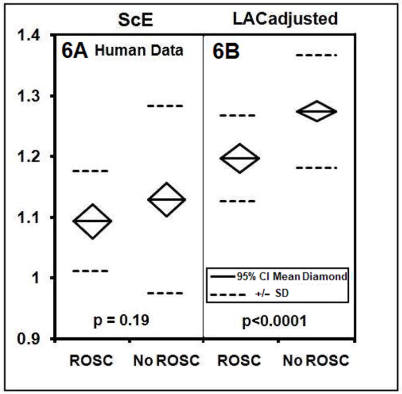
Fig. (6A). Results for human data: mean values of the ScE for the initial shock of VF by AED. The ROSC group has mean of 1.093 (SD +/− 0.083, n=36) and the No ROSC group has a mean of 1.128 (SD +/−0.1540, n=122, p=0.19). (6B): LACadjusted for the initial shock for VF by AED. The ROSC group has mean= 1.196 (SD +/−.071, n=36) and the No ROSC group has mean 1.273 (SD +/−.092, n=122, p < 0.0001).

Fig. 7.

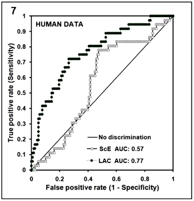
Fig. (7). ROC curves for the LAC for human data for first shock of VF with ROSC as the positive response has an AUC of 0.77 (ROSC; n=36, NO ROSC; n=122). The ROC curve for the ScE is also shown for comparison with AUC of 0.57.

DISCUSSION

Based on this evaluation of human and animal VF, the LAC is an effective method for assessing roughness in the VF waveform. At optimal recording rates of 1000 samples/second, the LAC enables estimation of VF duration in the swine model comparable to the ScE. A potential clinical advantage of the LAC over the ScE is that the LAC is not altered by recording rates less than 250 samples/second and therefore would retain its predictive characteristics in many current field-model AEDs. Indeed in the current investigation of human data derived from commercial AEDs, the LAC predicted ROSC substantially better than the ScE measure. Thus the LAC technique might enable discrimination of patients more likely to respond to immediate defibrillation from those who would benefit from CPR and other therapies prior to defibrillation. The primary advantage of the LAC (over the ScE) is that it could be used in currently available defibrillators to guide therapy.

It is interesting to note that the LAC shows changes analogous to the 3 phases of VF described by Weisfeldt and Becker [22]. With the LAC (Fig. 3A) there is an early down sloping period of VF less than 5 minutes in duration which temporally corresponds to the electrical phase. This is followed by a plateau until 9 minutes potentially representing a “circulatory” period during which CPR is effective in improving outcome. Following this is another down sloping period beyond 9 minutes that may correspond to the “metabolic” phase in which resuscitation becomes increasingly difficult. We speculate that once it becomes possible to detect and monitor which phase of VF is present through waveform analysis techniques, resuscitation may be tailored in a manner that is phase-targeted. In such a scenario, defibrillation would be delayed in a subset of patients while therapies such as CPR, drugs, and hypothermia would be applied until the monitored waveform measure attains an appropriate level such that defibrillation has an acceptable likelihood of ROSC.

LIMITATIONS

This study was a retrospective study. The ROSC outcome measure relied on a combination of an organized rhythm with audio and/or written confirmation of a spontaneous pulse. Although this combination is reasonable and practical given the clinical circumstances, the correct determination of ROSC can be challenging. The robustness of the LAC measure should be evaluated in prospective assessment using different populations. To this end, the optimal LAC cut-point that best directs care to immediate defibrillation versus alternate treatments (CPR) will need to be defined by further clinical experience. In the current human experience, the LAC had an AUC of 0.77 for predicting ROSC. Hence the LAC provides useful but imperfect prognostic information. As with other quantitative VF waveform measures, clinical use of the LAC would need to consider the LAC measurement characteristics (sensitivity and specificity) when implementing a resuscitation strategy. Moreover, clinical trials provide the best approach to determine the magnitude of survival benefit of any resuscitation strategy that uses quantitative VF measurement.

In summary, a new measure of the roughness of the VF waveform, the LAC, provides prognostic information regarding the duration of VF and the likelihood of ROSC under the recording conditions present in commercial defibrillators and represents an advance compared to the currently-available fractal dimension measure of VF waveform, the ScE. Potentially, iterative improvement in waveform prediction that combines advances in fractal dimension or ‘roughness’ measurement could be coupled with refinements in VF assessment based on frequency analysis and in turn translate into increased survival following VF cardiac arrest.

References

- 1.Cobb LA, Fahrenbruch C, Walsh T, Copass M, Olsufka M, Breskin M, Hallstrom A. Influence of cardiopulmonary resuscitation prior to defibrillation in patients with out-of-hospital ventricular fibrillation. JAMA. 1999;281(13):1182–8. doi: 10.1001/jama.281.13.1182. [DOI] [PubMed] [Google Scholar]
- 2.Wik L, Hansen TB, Fylling F, Steen T, Vaagnes P, Auestad BH, Steen PA. Delaying defibrillation to give basic cardiopulmonary resuscitation to patients with out-of-hospital ventricular fibrillation. JAMA. 2003;289(11):1389–95. doi: 10.1001/jama.289.11.1389. [DOI] [PubMed] [Google Scholar]
- 3.Vilke GM, Chan TC, Dunford JV, Metz M, Ochs G, Smith A, Fisher R, et al. The three-phase model of cardiac arrest as applied to ventricular fibrillation in a large, urban emergency medical services system. Resuscitation. 2004;64:341–346. doi: 10.1016/j.resuscitation.2004.09.011. [DOI] [PubMed] [Google Scholar]
- 4.Callaway CW, Menegazzi JJ. Waveform analysis of ventricular fibrillation to predict defibrillation. Current Opinion in Critical Care. 2005;11:192–199. doi: 10.1097/01.ccx.0000161725.71211.42. [DOI] [PubMed] [Google Scholar]
- 5.Dzwonczyk R, Brown CG, Werman HA. The median frequency of the ECG during ventricular fibrillation: its use in an algorithm for estimating the duration of cardiac arrest. IEEE Trans Biomed Eng. 1990;37:640–6. doi: 10.1109/10.55668. [DOI] [PubMed] [Google Scholar]
- 6.Brown CG, Dzwonszyk R. Signal analysis of the human electrocardiogram during ventricular fibrillation: frequency and amplitude parameters as predictors of successful countershock. Ann Emerg Med. 1996;27(2):184–8. doi: 10.1016/s0196-0644(96)70346-3. [DOI] [PubMed] [Google Scholar]
- 7.Berg RA, Hilwig RW, Kern KB, Ewy GA. Precountershock cardiopulmonary resuscitation improves ventricular fibrillation median frequency and myocardial readiness for successful defibrillation from prolonged ventricular fibrillation: a randomized, controlled swine study. Ann Emerg Med. 2002;40(6):563–70. doi: 10.1067/mem.2002.129866. [DOI] [PubMed] [Google Scholar]
- 8.Sherman LD, Callaway CW, Menegazzi JJ. Ventricular fibrillation exhibits dynamical properties and self-similarity. Resuscitation. 2000;47(2):163–73. doi: 10.1016/s0300-9572(00)00229-x. [DOI] [PubMed] [Google Scholar]
- 9.Sherman LD, Flagg A, Callaway CW, Menegazzi JJ, Hsieh M. Angular velocity: a new method to improve prediction of ventricular fibrillation duration. Resuscitation. 2004;60:79–90. doi: 10.1016/j.resuscitation.2003.07.001. [DOI] [PubMed] [Google Scholar]
- 10.Pernat AM, Weil MH, Tang W, et al. Optimizing timing of ventricular defibrillation. Circulation. 1999;100:1–313. doi: 10.1097/00003246-200112000-00019. [DOI] [PubMed] [Google Scholar]
- 11.Povoas HP, Weil MH, Tang W, Bisera J, Klouche K, Barbatsis A. Predicting the success of defibrillation by electrocardiographic analysis. Resuscitation. 2002;53:77–82. doi: 10.1016/s0300-9572(01)00488-9. [DOI] [PubMed] [Google Scholar]
- 12.Eilevstjonn J, Kramer-Johansen J, Sunde K. Shock outcome is related to prior rhythm and duration of ventricular fibrillation. Resuscitation. 2007;75:60–67. doi: 10.1016/j.resuscitation.2007.02.014. [DOI] [PubMed] [Google Scholar]
- 13.Eftestol T, Sunde K, Aase SO, Husoy JH, Steen PA. Predicting outcome of defibrillation by spectral-characterization and nonparametric classification of ventricular fibrillation in patients with out-of hospital cardiac arrest. Circulation. 2000;102:1523–9. doi: 10.1161/01.cir.102.13.1523. [DOI] [PubMed] [Google Scholar]
- 14.Strohmenger H, Eftestol T, Sunde K, Wenzel V, Mair M, Ulmer H, Lindner KH, Steen PA. The predictive value of ventricular fibrillation electrocardiogram signal frequency and amplitude variables in patients with out-of -hospital cardiac arrest. Anesth Analg. 2001;93:1428–33. doi: 10.1097/00000539-200112000-00016. [DOI] [PubMed] [Google Scholar]
- 15.Watson JN, Addison PS, Clegg GR, Holzer M, Sterz F, Robertson CE. Evaluation of arrhythmic ECG signals using a novel wavelet transform method. Resuscitation. 2000;43(2):121–127. doi: 10.1016/s0300-9572(99)00127-6. [DOI] [PubMed] [Google Scholar]
- 16.Watson JN, Uchaipichat N, Addison PS, Clegg GR, Robertson CE, Eftestol T, Steen PA. Improved prediction of defibrillation success for out-of-hospital VF cardiac arrest using wavelet transform methods. Resuscitation. 2004;63:269–275. doi: 10.1016/j.resuscitation.2004.06.012. [DOI] [PubMed] [Google Scholar]
- 17.Callaway CW, Sherman LD, Menegazzi JJ, Scheatzle MD. Scaling structure of electrocardiographic waveform during prolonged ventricular fibrillation in swine. Pacing Clin Electrophysiol. 2000;2:180–91. doi: 10.1111/j.1540-8159.2000.tb00799.x. [DOI] [PubMed] [Google Scholar]
- 18.Menegazzi JJ, Callaway CW, Sherman LD, Hostler DP, Wang HE, Fertig KC, Logue ES. Ventricular fibrillation scaling exponent can guide timing of defibrillation and other therapies. Circulation. 2004;109:926–931. doi: 10.1161/01.CIR.0000112606.41127.D2. [DOI] [PubMed] [Google Scholar]
- 19.Menegazzi JJ, Wang HE, Lightfoot CB, et al. Immediate defibrillation versus interventions first in a swine model of prolonged ventricular fibrillation. Resuscitation. 2003;59:261–270. doi: 10.1016/s0300-9572(03)00212-0. [DOI] [PubMed] [Google Scholar]
- 20.Callaway CW, Sherman LD, Mosesso VN, Dietrich TJ, Holt E, Clarkson C. Scaling exponent predicts defibrillation success for out-of-hospital ventricular fibrillation cardiac arrest. Circulation. 2001;103:1656–61. doi: 10.1161/01.cir.103.12.1656. [DOI] [PubMed] [Google Scholar]
- 21.Williams GP. Chaos theory tamed. Washington, DC: Joseph HenryPress; 1997. pp. 97–106. [Google Scholar]
- 22.Weisfeldt ML, Becker LB. Resuscitation after cardiac arrest: a 3-phase time-sensitive model. JAMA. 2002;288(23):3035–8. doi: 10.1001/jama.288.23.3035. [DOI] [PubMed] [Google Scholar]
Associated Data
This section collects any data citations, data availability statements, or supplementary materials included in this article.