

Abstract
In rodent hippocampus, neuronal activity is organized by a 6–10 Hz theta oscillation. The spike timing of hippocampal pyramidal cells with respect to the theta rhythm correlates with an animal's position in space. This correlation has been suggested to indicate an explicit temporal code for position. Alternatively, it may be interpreted as a byproduct of theta-dependent dynamics of spatial information flow in hippocampus. Here we show that place cell activity on different phases of theta reflects positions shifted into the future or past along the animal's trajectory in a two-dimensional environment. The phases encoding future and past positions are consistent across recorded CA1 place cells, indicating a coherent representation at the network level. Consistent theta-dependent time offsets are not simply a consequence of phase-position correlation (phase precession), because they are no longer seen after data randomization that preserves the phase-position relationship. The scale of these time offsets, 100–300 ms, is similar to the latencies of hippocampal activity after sensory input and before motor output, suggesting that offset activity may maintain coherent brain activity in the face of information processing delays.
Keywords: hippocampus, place cells, theta oscillation, phase precession, temporal coding, response latency
Introduction
The “temporal coding” hypothesis proposes that neurons use precise spike times, in addition to firing rates, to communicate information. An observation often cited in favor of this possibility is the hippocampal “phase precession” effect. During spatial behaviors, the hippocampus exhibits a regular 6–10 Hz “theta” oscillation. Both the firing rate of hippocampal place cells and their spike times with respect to the theta oscillation are correlated with an animal's location in space (O'Keefe and Dostrovsky, 1971; O'Keefe and Recce, 1993; Harris et al., 2002; Mehta et al., 2002). When an animal runs on a one-dimensional track, a place cell fires at a late phase of theta when the animal initially enters the place field, but firing advances to earlier phases as the animal traverses the field. In two-dimensional environments, the relationship of spike timing to the animal's position and head direction is less clear, but again an asymmetric precession from late to early phases is seen as the animal crosses the place field, whichever the direction of running (Skaggs et al., 1996; Harris et al., 2002).
These observations are typically interpreted within the temporal coding framework, to indicate that spike times of individual cells explicitly convey information about the animal's position to downstream cells (Jensen and Lisman, 2000; Huxter et al., 2003; Lengyel et al., 2003; O'Keefe and Burgess, 2005). A complementary viewpoint holds that the organization of spike times is a signature of ongoing computation taking place through the sequential activity of hippocampal cell assemblies within a theta cycle (Tsodyks et al., 1996; Hasselmo et al., 2002; Harris, 2005; Dragoi and Buzsaki, 2006). In support of this possibility, hippocampal spike times show greater coordination than expected from independent temporal coding of spatial location (Harris et al., 2003).
Here we set out to verify the hypothesis that, across the population of place cells, different phases within the same theta cycle encode positions offset into either the future or past along the rat's trajectory in a two-dimensional environment (see Fig. 1). Spiking activity of CA1 place cells was recorded in freely moving rats in an open field environment, and a succession of models predicting the activity of hippocampal place cells was fit to the spiking data. We found that spikes on different phases of theta are best predicted from the immediate future or immediate past location of the rat. Moreover, theta phases corresponding to “future” and “past” trajectory points are consistent across the population of place cells in CA1, suggesting a coherent representation of position across this hippocampal population. Although this phenomenon may be one of the mechanisms contributing to phase precession, we show that it is not simply a consequence of phase-position correlation, because randomized data in which the phase precession of the individual cells was retained did not show this behavior.
Figure 1.
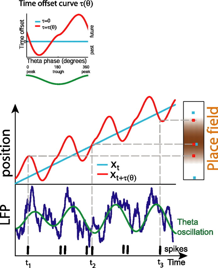
Position encoding with dynamic time offsets. Instantaneous trajectory xt (light blue) is “deformed” by the evolving theta phase of the local field potential (LFP; dark blue) according to the time offset curve τ(θ) (inset). The resulting trajectory xt + τ(θ) (red) is oscillating between future and past positions. When the rat approaches the place field (time t1), the corresponding place cell can only fire according to a future position that lies inside the place field; thus, spikes can only occur on a rising theta phase [see τ(θ) curve; inset]. While the rat traverses the place field (time t2), firing occurs at phases with small time offset, i.e., at values of theta near the trough. When the rat has left the place field (time t3), the cell can only fire according to a past position (inside the place field), hence on a falling theta phase.
Materials and Methods
Animals and recordings
Male Long–Evans rats (n = 3, five recording sessions) were implanted with four-shank 32-site silicon probes as described previously (Csicsvari et al., 2003). The animals were water restricted and trained to search for water droplets on a platform (1.8 × 1.8 m or 1 × 1.3 m). Head position and orientation were determined from two light-emitting diodes fixed on the head, monitored by an overhead camera with resolution 3.5 pix/cm. All experimental procedures were in accordance with Rutgers University guidelines. Extracellular spikes and instantaneous theta phase were extracted from the traces as described by Harris et al. (2002).
Computation of place fields
Place fields were computed as
 |
where x̃t = xt + τ(θt) is the trajectory [possibly altered by a theta-dependent time offset τ(θ)], ts are the spike times, φ(z)=exp(−|z|2/2σ;2d2), d is the largest side of the rectangular foraging area, and σ; is a smoothing parameter. For each considered cell, the parameter σ was computed to maximize the quality of prediction on the test set (see cross-validation) for the place field model without time offsets; the average value of σ was 0.038.
Cell selection criteria
Putative pyramidal cells were selected to satisfy the following three criteria: (1) average firing rate ≥0.6 Hz; (2) separation quality ≥18 (Schmitzer-Torbert et al., 2005); and (3) optimal smoothing parameter σ ≤ 0.06. A total of 85 recorded cells satisfied the above criteria (19, 17, 23, 12, and 14 in each respective session.)
Analyses
Cross-validation. We compare different models using the following cross-validation procedure. Each dataset was divided into five equal time intervals, yielding five different training/test set splits. For each split, four of the five time intervals were considered to be the “training set” (supplemental Fig. S1A, available at www.jneurosci.org as supplemental material), in which the parameters of each model were fit. The fitted models provided predictions for the instantaneous firing rate λ(t) on the “test set,” i.e., the remaining fifth time interval. Fit quality was evaluated based on log-likelihood
 |
of observing the spike train on the test set (here ts are the spike times on the test set) given the firing rate λ(t). The fit quality is defined as L = L(λ) − L(λ0), where λ0 is the firing rate prediction from the simplest model involving only the place field. To avoid bias in the selection of the test set (see the distributions for position, speed, and head direction in supplemental Fig. S1, available at www.jneurosci.org as supplemental material), this procedure was performed for all five combinations of training/test intervals. The fit quality L was averaged over all five choices of the test set.
Model fitting.
For the “place field model,” the instantaneous firing rate λ(t) was computed as λ(t) = F(x̃t), where x̃t = xt + τ(θt) is the (possibly time offset) trajectory. For the “global theta tuning model,” λ(t) = A(θt − μ,κ)F(x̃t), the parameters of the von Mises distribution A(θ−μ,κ) = exp(κcos(θ−μ))/2πI0(κ) were fit as
 |
where A1 is the ratio of Bessel functions A1(y) = I1(y)/I0(y) (Fisher, 1993), ts are the spike times, and Ns is the total number of spikes in the spike train. For the “phase field model,” λ(t) = A(θt − μ(x̃t),κ(x̃t))F(x̃t), the fields μ(x) and κ(x) were fit as
 |
 |
For the “head-direction-dependent phase field model,” λ(t) = A(θt − μ(Yt),κ(Yt))F(Yt), where Yt = (xt,HDt) and HDt is the instantaneous head direction, the fields F(y), μ(y), and κ(y) were computed as
 |
 |
where ψ(x,HD) = φ(x)exp(ρcosHD)2πI0(ρ), and the parameter ρ was computed to maximize the quality of prediction on the test set; the average value of ρ was 1.62.
For each considered cell and each appropriate model, constant time offsets were computed to maximize the similarity
 |
of the firing rate λ(t) to the spike train on the training set. The function Q(λ) is similar to log-likelihood but is more robust to noise (Itskov et al., 2008). The dynamic time offsets were computed by optimizing a three-parameter family of functions: τ(θ) = Bsin(sign(θ − θ0)|θ − θ0|βπ1−β) + τ0, where the values θ of the theta phase are measured in radians and span the interval (−π,π). Note that τ(θ) is a continuous (and periodic) function of θ as well as of all the other parameters. The three parameters B, θ0, and τ0 were fit for each individual cell to maximize the Q(λ), whereas β = 1.5 was chosen uniformly for all cells to maximize goodness of fit for the population. This particular parameterization was chosen because it provided the best prediction quality among a number of alternative parameterizations tested. We validated this choice by comparing the fits with the fits with a parameterization by six-point piecewise linear functions (supplemental Fig. S2, available at www.jneurosci.org as supplemental material). The piecewise linear parameterization allows for a significantly more general shape of τ(θ); in particular, it does not impose any bimodality. The fits by piecewise linear functions were in very good agreement with the three-parameter family we used.
Inclusion of spike history dependence.
To ensure that our results are not affected by spike history dependence (Barbieri et al., 2001; Treves, 2004), we computed the timescales of neural adaptation in the recorded cells and also fit the model with theta-dependent time offsets and spike history dependence. For each cell, a place field model λ(t) = g(wt)F(xt) was fit. Here,
 |
is a variable reflecting the spiking history at each time t, δ is a time scale of neural adaptation, ts are the spike times, and
 |
describes the modulation of the instantaneous firing rate by the spiking history wt ([z]+ = z if z ≥ 0, and [z]+ = 0 if z < 0). The rational function form for g(w) was chosen because it provided good cross-validated fits compared with other considered parametric families (such as a polynomial times an exponential in w). The thresholding ensures that λ(t) is always non-negative. For each considered δ, the coefficients (a, b, c, d) were fit on the training set, and the quality of fit was evaluated on the test set. An optimal timescale δ was fit for each cell to maximize the quality of fit on the test set. Most of the considered cells exhibited timescale δ < 11 ms (supplemental Fig. S3C, available at www.jneurosci.org as supplemental material). Note that the time delay between theta phases with future and past time offsets is on the order of 50 ms. We also fit a model that incorporated both spike history dependence and variable time offsets: λ(t) = g(wt)F(xt + τ(θ)). As is expected from the small timescale of neural adaptation, the theta-dependent time offsets do not differ significantly from those computed without neural adaptation (supplemental Fig. S3D, available at www.jneurosci.org as supplemental material).
Simulation.
For each cell that showed preference for dynamic time offsets in the phase field model type, a head direction-dependent baseline (no time offsets) phase field model was fit to the data on the entire recording session. The model parameters were used to generate a spike train from the rate of an inhomogeneous Poisson process according to that model using the phase θt and the trajectory and head direction information Yt of the real data. Time offset curves τ(θ) were fit for n = 62 real and corresponding simulated cells.
Circular variance of future theta phase.
For each set (real and simulated) of fitted curves τj(θ), j = 1,… ,N, the future phases were computed as θj = arg max τj(θ), and the circular variance was computed as
 |
Results
We investigated the relationship between the firing of place cells and the phase of theta oscillation using a model selection approach. By a model, we mean a rule that predicts, from the rat's trajectory xt and instantaneous theta phase θt, the instantaneous firing rate λ(t) of a given place cell. In other words, a model is a prescription F for computing λ(t) = F(xt, θt). The success with which each model could predict the spike train of a neuron was evaluated using a cross-validation procedure (see Materials and Methods). This cross-validation procedure penalizes models with extraneous parameters; only meaningful additional parameters improve the quality of prediction.
As a preliminary step, we fit a simple place field model, in which the instantaneous firing rate of a place cell is determined only by the instantaneous position of the rat as λ(t) = F(xt) [we refer to the function F(x) as the place field]. As expected, for all 85 cells satisfying our criteria for unit isolation quality and firing rate (see Materials and Methods), this prediction was significantly better than a prediction of constant firing rate. Next, we examined position encoding with “constant time offsets.” Although the usual place field model uses the instantaneous position xt, the hippocampus may better encode the animal's position with a certain time shift into the past or future. The appropriate correction for the place field model would be λ(t) = F(xt + τ), where τ is the constant time offset. For each place cell, the constant time offset τ was chosen automatically to provide the best fit. Similar to previous work (Muller and Kubie, 1989), this model provided a better fit than the simple (zero offset) place field model in 50 of 85 considered place cells, with an average measured time offset of 62 ms into the future.
To investigate the dependence of position encoding on theta phase, we began by considering the theta dependence of time offsets. This leads us to a place field model λ(t) = F(x̃t) with a time-deformed trajectory x̃t = xt + τ(θt) (Fig. 1), determined by a “dynamic time offset” τ(θ). For every value θ of the theta phase, we associate a time offset τ(θ); the set of all time offsets for all values of θ forms a curve (Fig. 1, inset). In particular, we allow that different spikes from the same cell may correspond to either the future or past position of the rat, depending on the phase of theta at which the spikes occurred. For each place cell, we tested for dynamic time offsets by comparing such a model with the constant time offset model. We found that the dynamic time offsets model fit better for 84% of cells (p < 3 × 10⁻⁷ on paired t test) (Fig. 2B).
Figure 2.

The majority of CA1 place cells exhibit dynamic time offset curves whose dependence on theta is consistent across the population. A, Improvement in quality of prediction for three baseline models compared with the place field model. The quality of fit L(λ) (see Materials and Methods) was evaluated for each model (place field, global theta tuning, phase field, and head direction-dependent phase field). The bars represent the average (across the population of cells) difference L = L(λ) − L(λ0) in quality of fit between each baseline model and the place field model. Error bars represent SEs. B, For each cell and each model class (place field, global theta tuning, phase field, and head direction-dependent phase field), the quality of prediction L was computed for the model fit with no time offsets (blue), constant time offsets (green), and dynamic time offsets (red). The bars represent the average (across the population of cells) goodness of fit L. For the majority of cells (84, 85, 72, and 68% in each respective model class), the cell firing was better fit with dynamic time offsets than with constant time offsets. The p values are for the paired t test, testing the null hypothesis that the quality of fit was not improved for the dynamic time offset model compared with the next best model in the same model class. C, Dynamic time offset curves τ(θ) for the phase field model class, fit from all cells that showed preference for the dynamic time offset model. Curves fit for the other model classes were similar to shown. Note that positive (future) time offsets occur on rising theta phase, and negative (past) time offsets occur on falling theta phase. D, Maxima (filled diamonds) and minima (open diamonds) of the curves in C. Remarkably, future/past phases are consistent across the population of cells [circular variance V = 0.1 for future phases (see Materials and Methods)].
At this point, one might argue that the reason why the dynamic time offset model performs best is because it is the only model using theta phase in its prediction. Would the dynamic time offset model still outperform constant time offsets if theta modulation were explicitly included in the underlying place field model? To address this question, we considered three additional sequentially more complex “baseline” (i.e., no time offset) models that incorporate theta modulation directly. The first baseline model introduces a (global) “theta tuning curve” A for each cell, such that the firing rate is given by λ(t) = A(θt − μ,κ)F(xt), where μ and κ are constants, and A(θt − μ,κ) is the von Mises probability density function (Fisher, 1993) of the theta phase for individual spikes (here μ is the preferred phase of the cell, and κ controls the variance). The second baseline model allows the preferred phase and variance to depend on position: λ(t) = A(θt − μ(xt),κ(xt))F(xt). One can think of μ(x) as a “phase field” that associates a preferred phase to each location in space. The third model allows the place field and the phase field to also depend on the head direction.
We compared the performance of each baseline model relative to the place field model and then compared the improvement of each baseline model with constant versus dynamic time offsets. As expected, incorporating theta tuning curves, phase fields, and head direction directly into the baseline model improved performance (Fig. 2A); however, in each case, most cells (84, 85, 72, and 68% in each respective model class) were best described by the model with dynamic time offsets (Fig. 2B). This suggests that phase-dependent time offsets improve spike train prediction regardless of how we include theta dependence in the underlying model. Our conclusions are also not affected by inclusion of spiking history dependence (see Materials and Methods) (supplemental Fig. S3, available at www.jneurosci.org as supplemental material).
Analysis of the shape of the fitted curves τ(θ) revealed striking coherence in the trajectory encoding of the recorded cells with offsets furthest into the past and future occurring at the falling (74 ± 45° after the peak) and rising (68 ± 31° before the peak) phases of the CA1 pyramidal layer theta rhythm (Fig. 2C,D). This correlation suggests that the CA1 population coherently represents the rat's future and past positions on the same phases of theta.
We therefore observe that the spike trains of CA1 pyramidal cells are best predicted with dynamic time offsets. Such a phenomenon had been hypothesized from the existence of phase/position correlation (Skaggs et al., 1996). Are the observed dynamic time offsets a simple consequence of phase/position correlation (phase precession)? To answer this question, we used our original data to construct a simulated dataset that preserves the phase/position correlation for each original cell. If the observed dynamic time offsets are also present in the simulated data, it would indicate that they are a simple consequence of phase precession; if not, it would suggest that they reflect a more elemental principle organizing hippocampal spike times. To capture the phase/position correlation in the original data, we fit a variant of the phase field model predicting the place field F of each cell and preferred phase μ as a function of the animal's position and head direction; head direction information is necessary because, in two-dimensional environments, the theta phase at any location varies with the angle of approach into the place field (Skaggs et al., 1996). From this model, a simulated dataset was generated by sampling from an inhomogeneous Poisson process with rate determined by the rat's instantaneous location, head direction, and theta phase (see Materials and Methods). As expected, the simulated spike trains exhibited phase precession similar to that in the original observed spike trains (Fig. 3A,C). However, the consistent dynamic time offsets seen in the original data were replaced by an incoherent and small-amplitude pattern in simulated data (Fig. 3E–G) [in the real data, the circular variance (see Materials and Methods) for the future phase was V = 0.1, with median amplitude of τ(θ) 347 ms; in simulated data, V = 0.6, and median amplitude was 37 ms]. We therefore conclude that dynamic time offsets (with different phases of theta corresponding to immediate past/future position consistently across the population) is a distinct and perhaps more elementary phenomenon than phase precession.
Figure 3.
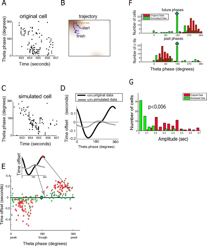
Theta phase precession does not explain observed dynamic time offsets. A, Theta phases of spikes versus time for a recorded cell while the rat was traversing a place field along the trajectory shown in B. B, Trajectory for the time interval in A together with the place field for that cell. C, We fit a head direction-dependent phase field model from the entire recording (∼40 min) of the original cell in A. The resulting model parameters were then used to simulate a spike train from the trajectory, head direction, and theta phase information of the real data. The spike train generated from this model exhibits a similar pattern of phase precession as the real spike train. Shown are the theta phases of spikes versus time for the same run across the place field as in A. D, Dynamic time offsets for the phase field model were fit for the original and simulated cells. Graphs of τ(θ) fit for the original (black) and simulated (gray) cells. Although the simulated cell exhibits a pattern of phase precession similar to that of the original cell, it does not exhibit similar dynamic time offsets. E, Comparison of dynamic time offsets across the population of real and simulated cells. The scatter plot shows the maxima (filled diamonds) and minima (open diamonds) of the time offset curves τ(θ) for each real (red) and simulated (green) cell. For simulated cells, dynamic time offsets are destroyed although phase precession is preserved, indicating that they are not a simple consequence of phase precession. Note that 19 of 62 simulated cells were best fit with zero τ(θ) (big green diamond in the middle). All curves τ(θ) are fit for the phase field model class. F, Distribution of future/past phases for the recorded (red) and the simulated (green) cells. Future/past phases are consistent across the population of real cells but not for simulated cells. Simulated cells best fit with a zero-amplitude τ(θ) were assigned future and past time offset phases at 180° (bars below green diamonds). G, Distribution of the amplitudes of the dynamic time offsets for the recorded (red) and the simulated (green) cells. Whereas the median amplitude for the real cells was 347 ms, the median amplitude for the simulated cells was 37 ms, i.e., almost 10-fold smaller. The displayed p value is for the paired t test, testing the null hypothesis that these two distributions have the same mean.
Discussion
We find that the activity of a CA1 population is best predicted from the rat's location at a time offset into the past or future, depending on the phase of the theta cycle. The dependence of this offset on theta phase (measured in the CA1 pyramidal layer) was consistent across the population, with a mean negative offset of 161 ms at 74° after the peak (the falling phase) and a mean positive offset of 196 ms at 292° (the rising phase). On the falling phase, the population therefore best reflects the animal's location at the end of the second-to-last theta cycle; by the time the rising phase has arrived, population activity reflects a prediction of the animal's location approximately two theta cycles into the future. These observations are compatible with, but not a consequence of, the dependence of firing phase on location (phase precession); the observed dynamic time offsets were not seen in simulated datasets in which the relationship between spiking phase, location, and head direction was preserved. Conversely, it is quite conceivable that the observed dynamic time offsets could contribute to the phenomenon of phase precession.
Environmental signals are conveyed to the hippocampus by the neocortex, and the majority of hippocampal output returns to neocortex, suggesting that a function of the hippocampus is to return information to the neocortex in response to a pattern received as input. The theta rhythm may serve as a timer of this process, with the “reset” provided by the relative silence at the peak of each theta wave allowing a new cycle of encoding and retrieval to occur (Hasselmo, 2005). Our findings are suggestive of the following interpretation. Activity at the start of the theta cycle (the falling phase) reflects cortical input of a primarily sensory nature. This input is dependent on the animal's location, but, because of the delays involved in traversing multiple cortical regions, it is best correlated with the animal's position as it was shortly in the past. By the end of the theta cycle (the rising phase), CA1 activity represents the results of intrahippocampal computations, which may serve a variety of purposes, perhaps including providing context for the interpretation of new sensory data, or the production of motor outputs. Because the return signaling to sensory and motor areas will again take time, hippocampal output must be relevant to the world as it will be shortly into the future. The timescales of a few hundred milliseconds that we find for the past and future predictions are consistent with the timing of hippocampal activity after sensory stimuli and before movement onsets (Shinba, 1999; Tesche and Karhu, 1999). The highly structured spike timing patterns seen during the theta cycle may thus reflect a mechanism of maintaining coherent brain activity in the face of processing delays.
Footnotes
This work was supported by National Institutes of Health Grants R01MH073245, NS34994, and NS43157. V.I. was supported by the Swartz Foundation, E.P. was supported by the Patterson Trust, K.M. was supported by the Uehara Foundation, and K.D.H. was supported by the Sloan Foundation.
References
- Barbieri R, Quirk MC, Frank LM, Wilson MA, Brown EN. Construction and analysis of non-Poisson stimulus-response models of neural spiking activity. J Neurosci Methods. 2001;105:25–37. doi: 10.1016/s0165-0270(00)00344-7. [DOI] [PubMed] [Google Scholar]
- Csicsvari J, Henze DA, Jamieson B, Harris KD, Sirota A, Bartho P, Wise KD, Buzsaki G. Massively parallel recording of unit and local field potentials with silicon-based electrodes. J Neurophysiol. 2003;90:1314–1323. doi: 10.1152/jn.00116.2003. [DOI] [PubMed] [Google Scholar]
- Dragoi G, Buzsaki G. Temporal encoding of place sequences by hippocampal cell assemblies. Neuron. 2006;50:145–157. doi: 10.1016/j.neuron.2006.02.023. [DOI] [PubMed] [Google Scholar]
- Fisher NI. Statistical analysis of circular data. Cambridge, UK: Cambridge UP; 1993. [Google Scholar]
- Harris KD. Neural signatures of cell assembly organization. Nat Rev Neurosci. 2005;6:399–407. doi: 10.1038/nrn1669. [DOI] [PubMed] [Google Scholar]
- Harris KD, Henze DA, Hirase H, Leinekugel X, Dragoi G, Czurko A, Buzsaki G. Spike train dynamics predicts theta-related phase precession in hippocampal pyramidal cells. Nature. 2002;417:738–741. doi: 10.1038/nature00808. [DOI] [PubMed] [Google Scholar]
- Harris KD, Csicsvari J, Hirase H, Dragoi G, Buzsaki G. Organization of cell assemblies in the hippocampus. Nature. 2003;424:552–556. doi: 10.1038/nature01834. [DOI] [PubMed] [Google Scholar]
- Hasselmo ME. What is the function of hippocampal theta rhythm? Linking behavioral data to phasic properties of field potential and unit recording data. Hippocampus. 2005;15:936–949. doi: 10.1002/hipo.20116. [DOI] [PubMed] [Google Scholar]
- Hasselmo ME, Bodelon C, Wyble BP. A proposed function for hippocampal theta rhythm: separate phases of encoding and retrieval enhance reversal of prior learning. Neural Comput. 2002;14:793–817. doi: 10.1162/089976602317318965. [DOI] [PubMed] [Google Scholar]
- Huxter J, Burgess N, O'Keefe J. Independent rate and temporal coding in hippocampal pyramidal cells. Nature. 2003;425:828–832. doi: 10.1038/nature02058. [DOI] [PMC free article] [PubMed] [Google Scholar]
- Itskov V, Curto C, Harris KD. Valuations for spike train prediction. Neural Comput. 2008;20:644–667. doi: 10.1162/neco.2007.3179. [DOI] [PubMed] [Google Scholar]
- Jensen O, Lisman JE. Position reconstruction from an ensemble of hippocampal place cells: contribution of theta phase coding. J Neurophysiol. 2000;83:2602–2609. doi: 10.1152/jn.2000.83.5.2602. [DOI] [PubMed] [Google Scholar]
- Lengyel M, Szatmary Z, Erdi P. Dynamically detuned oscillations account for the coupled rate and temporal code of place cell firing. Hippocampus. 2003;13:700–714. doi: 10.1002/hipo.10116. [DOI] [PubMed] [Google Scholar]
- Mehta MR, Lee AK, Wilson MA. Role of experience and oscillations in transforming a rate code into a temporal code. Nature. 2002;417:741–746. doi: 10.1038/nature00807. [DOI] [PubMed] [Google Scholar]
- Muller RU, Kubie JL. The firing of hippocampal place cells predicts the future position of freely moving rats. J Neurosci. 1989;9:4101–4110. doi: 10.1523/JNEUROSCI.09-12-04101.1989. [DOI] [PMC free article] [PubMed] [Google Scholar]
- O'Keefe J, Burgess N. Dual phase and rate coding in hippocampal place cells: theoretical significance and relationship to entorhinal grid cells. Hippocampus. 2005;15:853–866. doi: 10.1002/hipo.20115. [DOI] [PMC free article] [PubMed] [Google Scholar]
- O'Keefe J, Dostrovsky J. The hippocampus as a spatial map. Preliminary evidence from unit activity in the freely-moving rat. Brain Res. 1971;34:171–175. doi: 10.1016/0006-8993(71)90358-1. [DOI] [PubMed] [Google Scholar]
- O'Keefe J, Recce ML. Phase relationship between hippocampal place units and the EEG theta rhythm. Hippocampus. 1993;3:317–330. doi: 10.1002/hipo.450030307. [DOI] [PubMed] [Google Scholar]
- Schmitzer-Torbert N, Jackson J, Henze D, Harris K, Redish AD. Quantitative measures of cluster quality for use in extracellular recordings. Neuroscience. 2005;131:1–11. doi: 10.1016/j.neuroscience.2004.09.066. [DOI] [PubMed] [Google Scholar]
- Shinba T. Neuronal firing activity in the dorsal hippocampus during the auditory discrimination oddball task in awake rats: relation to event-related potential generation. Brain Res Cogn Brain Res. 1999;8:241–250. doi: 10.1016/s0926-6410(99)00026-9. [DOI] [PubMed] [Google Scholar]
- Skaggs WE, McNaughton BL, Wilson MA, Barnes CA. Theta phase precession in hippocampal neuronal populations and the compression of temporal sequences. Hippocampus. 1996;6:149–172. doi: 10.1002/(SICI)1098-1063(1996)6:2<149::AID-HIPO6>3.0.CO;2-K. [DOI] [PubMed] [Google Scholar]
- Tesche CD, Karhu J. Interactive processing of sensory input and motor output in the human hippocampus. J Cogn Neurosci. 1999;11:424–436. doi: 10.1162/089892999563517. [DOI] [PubMed] [Google Scholar]
- Treves A. Computational constraints between retrieving the past and predicting the future, and the CA3-CA1 differentiation. Hippocampus. 2004;14:539–556. doi: 10.1002/hipo.10187. [DOI] [PubMed] [Google Scholar]
- Tsodyks MV, Skaggs WE, Sejnowski TJ, McNaughton BL. Population dynamics and theta rhythm phase precession of hippocampal place cell firing: a spiking neuron model. Hippocampus. 1996;6:271–280. doi: 10.1002/(SICI)1098-1063(1996)6:3<271::AID-HIPO5>3.0.CO;2-Q. [DOI] [PubMed] [Google Scholar]