Using Markov models to simulate electron spin resonance spectra from molecular dynamics trajectories

Abstract

Simulating electron spin resonance (ESR) spectra directly from molecular dynamics simulations of a spin labeled protein necessitates a large number (hundreds or thousands) of relatively long (hundreds of ns) trajectories. To meet this challenge, we explore the possibility of constructing accurate stochastic models of the spin label dynamics from atomistic trajectories. A systematic, two-step procedure, based on the probabilistic framework of hidden Markov models, is developed to build a discrete-time Markov chain process that faithfully captures the internal spin label dynamics on time scales longer than about 150 ps. The constructed Markov model is used both to gain insight into the long-lived conformations of the spin label and to generate the stochastic trajectories required for the simulation of ESR spectra. The methodology is illustrated with an application to the case of a spin labeled poly-alanine alpha helix in explicit solvent.

I. INTRODUCTION

Electron spin resonance (ESR) spectra are rich in information that can be related to the structure and function of the spin labeled biomolecule. Nonetheless, inferring the molecular detail from the spectra is difficult due to the complexity introduced by the internal dynamics of the spectroscopic reporter. A thorough understanding of the conformational freedom and dynamics of the spin label, therefore, is highly desirable.

In a previous study¹ (‘paper I’ from now on), we performed molecular dynamics (MD) simulations of a fully solvated, poly-alanine α-helix containing one spin labeled cysteine residue at its central position: the most commonly used “side chain” R1, which results from linking the spin label MTSSL to a cysteine through a disulfide bond. This system was chosen as an idealized model of R1 at a solvent-exposed helix surface site in proteins. Due to the relatively small size of the system, we were able to simulate 18 independent trajectories, each extending for 100 ns. In spite of the reasonably long duration of the simulations, each individual trajectory failed to exhaustively sample all the conformations that were accessible to the spin label. As a result, the times that the R1 was observed to spend in its various conformations do not necessarily reflect the correct state probabilities, but likely depend on the starting conformations. On the other hand, when taken together, the trajectories seemed to explore a significant realm of conformational possibilities. Even the disulfide torsion angle with an energy barrier of 7 kcal/mol² was observed to make 10 transitions between its two stable conformations. There are compelling reasons to believe that the combined information from all the simulations ought to provide a good estimate of the populations of the various conformations and the rates of exchange between them. The issue begs for a robust analysis method to extract this information from a collection of MD trajectories.

An important ansatz to proceed with such an analysis is that during its evolution the spin label side chain “forgets” its past over some relatively short time scale. Mathematically, this suggests that the R1 dynamics can be modeled as a stochastic Markov jump process. The main idea is that many independent trajectories can be used to estimate conditional (transition) probabilities, even though each trajectory does not necessarily reflect the correct equilibrium probabilities. To this end, the detailed dynamics of the MD trajectories has to be mapped to a discrete-state Markov jump model, the state-to-state transition probability matrix (TPM) of which needs to be determined. The equilibrium probabilities of the various states are then calculated from the TPM, rather than from the fraction of their occurence in the trajectories. Once its parameters have been properly estimated, the so-constructed Markov model should allow for the generation of arbitrarily long stochastic trajectories, which can then be used to simulate ESR spectra in the time domain.

The outline of the paper is as follows: In Section II we analyze the dynamics of a spin system coupled to a classical bath, where the latter is assumed to exchange rarely between a number of discrete states and to equilibrate quickly inside each of the states. A two step procedure that aims to construct Markov models with the desired separation of time scales from the MD trajectories of a spin label is presented. In Section III, Markov models with different numbers of states are built from the MD trajectories of R1 at a poly-alanine α-helix. The resulting models are used to elucidate the various time scales associated with the internal spin label dynamics and to study the conformational changes that they correspond to. ESR spectra at three different frequencies are simulated from the trajectories generated by these models and compared with spectra simulated directly from the MD trajectories.¹ The implications of the results are discussed in Section IV and our conclusions are given in Section V. The appendix contains additional technical details.

II. THEORY AND METHODS

A. ESR spectra and stochastic dynamics

1. Stochastic Liouville equation background

The stochastic Liouville equation (SLE) introduced by Kubo^3–5 describes the dynamics of a quantal system coupled to a classical bath, where the dynamics of the bath is modeled by a stochastic process. The use of the SLE in the simulation of ESR spectra has been pioneered by Freed and co-workers.^6,7 A basic assumption of SLE theories is that the classical degrees of freedom are not influenced by the quantum dynamics. This approximation is justified for most phenomena involving magnetic resonance of electronic and nuclear spins.^8–10 Although additional considerations to the standard SLE are required to ensure relaxation of the spins to thermal equilibrium,¹⁰ this issue will not be considered here since the dephasing of the spins is the main contributor to T₂ relaxation phenomena that are our main interest.

Consider a quantal system coupled to an N-state, continuous-time Markov chain process. Let X(t) be a random variable indicating the state of the chain at time t. The probabilities p_i(t) = P{X(t) = i}, to observe the chain in state i at time t, form the vector p(t) = [p_i(t)], whose evolution is governed by the Master equation

$${\stackrel{.}{p}}_j\left(t\right)=\sum _{i=1}^N{p}_i\left(t\right)Q_{ij}.$$ (1)

The matrix Q = [Q_ij], referred to as the “rate matrix”, is the generator of the chain. Its off-diagonal entries are larger or equal to zero. For a conservative process, its diagonal elements are negative and given as¹¹

$$Q_{ii}=-\sum _{j\ne i}{Q}_{ij},$$ (2)

and are directly related to the lifetime ν_i of each state,

$${\nu }_i=-1∕Q_{ii}.$$ (3)

The stationary probability distribution of the chain π, is the left eigenvector of Q with eigenvalue zero. For a system in thermal equilibrium, π and Q are in detailed balance,

$${\pi }_i{Q}_{ij}={\pi }_j{Q}_{ji}.$$ (4)

This condition implies that Q can be transformed to a symmetric form by a similarity transformation with the matrix $D=\left[\sqrt{{\pi }_i}{\delta }_{ij}\right]$, thus all the eigenvalues of Q are real. When written as −1/τ_i, the nonzero eigenvalues give the relaxation time scales τ_i of the stochastic dynamics generated by Q. Note that τ_i ≠ ν_i.

The density operator of the quantal system, |ρ(t)〉〉, written as a Liouville space vector,¹² obeys the Liouville-von Neumann equation

$$\mid \stackrel{.}{\rho }\left(t\right)⟫=-\mathrm{i}{\check{L}}_{X\left(t\right)}\mid \rho \left(t\right)⟫,$$ (5)

in which the dependence of the Liouvillian on the state of the Markov chain is denoted as a subscript. (The inverted caret indicates that the Liouvillian is a Liouville space operator, i.e. a superoperator; the dot indicates differentiation with respect to time.) The SLE for this coupled quantum-classical system is an evolution equation for^3,4

$$\mid u_i\left(t\right)⟫=\mathbb{E}\{\mid \rho \left(t\right)⟫\mid X\left(t\right)=i\},$$ (6)

the expectation of the density matrix at time t given that currently X(t) = i. It reads^3,4

$$\mid {\stackrel{.}{u}}_j\left(t\right)⟫=-\mathrm{i}{\check{L}}_j\mid u_j\left(t\right)⟫+\sum _i{Q}_{ij}\mid u_i\left(t\right)⟫.$$ (7)

When X(0) is chosen from the equilibrium probability density π, the initial condition of eq (7) is

$$\mid u_i\left(0\right)⟫=\mid \rho \left(0\right)⟫{\pi }_i.$$ (8)

Notice that initially |u_i(t)〉〉 is separable in its classical and quantum parts.

For a bath which is modeled by a continuous stochastic process Y(t), the probability density p(y, t) is taken to satisfy a Fokker-Planck equation¹³

$${\partial }_{t}p(y,t)=\mathcal{G}p(y,t),$$ (9)

with stationary solution π(y). (∂_t denotes partial derivative with respect to t.) The differential operator $\mathcal{G}$ acts on the variable y. In such cases, the SLE becomes^3,4,10

$${\partial }_t\mid u(y,t)⟫=-\mathrm{i}\check{L}\left(y\right)\mid u(y,t)⟫+\mathcal{G}\mid u(y,t)⟫$$ (10)

with initial condition

$$\mid u(y,0)⟫=\mid \rho \left(0\right)⟫\pi \left(y\right).$$ (11)

2. Eliminating the fast intrastate dynamics

When different components of the classical dynamics evolve on well separated time scales one can formally eliminate the fast dynamics.¹⁴ For example, the dynamics of a given spin label can be viewed as a superposition of fast intrastate dynamics Y in a given state X = j, and much slower exchanges between the states. Symbolically, this can be written as^15–17

$$\stackrel{.}{Y}\left(t\right)=\frac{1}{∊}g(X\left(t\right),Y\left(t\right)),\stackrel{.}{X}\left(t\right)=f\left(X\left(t\right)\right),$$ (12)

where ε is a small parameter and the functions f and g are O(1) in ε. Clearly, for small ε, Y varies on a faster time scale than X. In eq (12) it is assumed for simplicity that the exchanges do not depend on the intrastate dynamics, thus f is independent of Y. Associated with this system of evolution equations is a Fokker-Planck-Master equation

$${\partial }_t{p}_j(y,t)=\frac{1}{∊}{\mathcal{G}}_j{p}_j(y,t)+\sum _i{p}_i(y,t)Q_{ij}$$ (13)

for the joint probability density p_i(y, t). The operator ${\mathcal{G}}_j$ acts only on the variable y but depends on the state j of the Markov chain. There is a different operator (with different diffusion tensor and ordering potential, for example) for each j. Its exact form is not important for the purposes of our discussion. Suffice it to say that π(y|j) that satisfies the condition

$${\mathcal{G}}_j\pi (y\mid j)=0$$ (14)

is the equilibrium probability density of Y for a given state j.

Coupling the classical processes in eq (12) to the quantal dynamics (cf. eq (5))

$$\mid \stackrel{.}{\rho }\left(t\right)⟫=-\mathrm{i}{\check{L}}_{X\left(t\right)}\left(Y\left(t\right)\right)\mid \rho \left(t\right)⟫,$$ (15)

one obtains the SLE

$$\begin{array}{cc}\hfill {\partial }_t\mid u_j(y,t)⟫=& \left(-\mathrm{i}{\check{L}}_j\left(y\right)+\frac{1}{∊}{\mathcal{G}}_j\right)\mid u_j(y,t)⟫\hfill \\ \hfill & +\sum _i{Q}_{ij}\mid u_i(y,t)⟫\hfill \end{array}$$ (16)

with initial condition

$$\mid u_i(y,0)⟫=\mid \rho \left(0\right)⟫{\pi }_i\left(y\right).$$ (17)

Here π_i(y) is the joint equilibrium probability density corresponding to eq (13). We look for a solution of the SLE in the form¹⁷

$$\mid u⟫=\mid u^{\left(0\right)}⟫+∊\mid u^{\left(1\right)}⟫+{∊}^2\mid u^{\left(2\right)}⟫+\cdots ,$$ (18)

with initial conditions

$$\begin{array}{cc}\hfill \mid u_i^{\left(0\right)}(y,0)⟫& =\mid u_i(y,0)⟫\hfill \\ \hfill \mid u_i^{\left(k\right)}(y,0)⟫& =0,k\ge 1.\hfill \end{array}$$ (19)

Substituting in eq (16) and collecting terms with equal power of ε leads to the hierarchy of equations

$${∊}^{-1}:{\mathcal{G}}_j\mid u_j^{\left(0\right)}(y,t)⟫=0,$$ (20a)

$$\begin{array}{cc}\hfill {∊}^0:{\mathcal{G}}_j\mid u_j^{\left(1\right)}(y,t)⟫& =({\partial }_t+\mathrm{i}{\check{L}}_j\left(y\right))\mid u_j^{\left(0\right)}(y,t)⟫\hfill \\ \hfill & -\sum _i{Q}_{ij}\mid u_i^{\left(0\right)}(y,t)⟫,\cdots .\hfill \end{array}$$ (20b)

The first equation implies that $\mid u_j^{\left(0\right)}(y,t)⟫$ is in the null space of ${\mathcal{G}}_j$. From eq (14) it follows that

$$\mid u_j^{\left(0\right)}(y,t)⟫=\pi (y\mid j)\mid h_j\left(t\right)⟫,$$ (21)

where h_j(t) is arbitrary. Let us define the operator^17–19

$$\mathcal{P}{a}_j\left(y\right)\equiv \pi (y\mid j)\int a_j\left(y\right)\mathrm{d}y,$$ (22)

which projects onto the null space of ${\mathcal{G}}_j$ by mapping a general function of (j, y) into a function of j times π(y|j). With this, the requirement that u⁽⁰⁾ is in the null space of ${\mathcal{G}}_j$ translates into $\mathcal{P}{u}^{\left(0\right)}=u^{\left(0\right)}$. It is not hard to see that ${\mathcal{PG}}_j$ = ${\mathcal{G}}_j\mathcal{P}$ = 0. Acting with $\mathcal{P}$ on both sides of the second equation in the hierarchy gives

$$\begin{array}{cc}\hfill {\partial }_t\mid u_j^{\left(0\right)}(y,t)⟫=& -\mathrm{i}\mathcal{P}{\check{L}}_j\left(y\right)\mid u_j^{\left(0\right)}(y,t)⟫\hfill \\ \hfill & +\sum _i{Q}_{ij}\mid u_i^{\left(0\right)}(y,t)⟫.\hfill \end{array}$$ (23)

Using eqs (21) and (22), the first term on the right hand side of the equality becomes

$$\mathcal{P}{\check{L}}_j\left(y\right)\mid u_j^{\left(0\right)}(y,t)⟫={\overline{\check{L}}}_j\mid u_j^{\left(0\right)}(y,t)⟫,$$ (24)

where

$${\overline{\check{L}}}_j\equiv \int {\check{L}}_j\left(y\right)\pi (y\mid j)\mathrm{d}y$$ (25)

is the Liouvillian for state j averaged over the equilibrium probability of the fast dynamics inside the state. The physical implication is that the process Y relaxes to its equilibrium distribution before X has time to change. As a result, eq (23) together with its initial condition can be viewed as the SLE corresponding to the system of equations

$$\stackrel{.}{X}\left(t\right)=f\left(X\left(t\right)\right),\mid \stackrel{.}{\rho }\left(t\right)⟫=-\mathrm{i}{\overline{\check{L}}}_{X\left(t\right)}\mid \rho \left(t\right)⟫.$$ (26)

Thus, to lowest order, one can replace the instantaneous Liouvillian with its average over the current state of the Markov chain. Below, we use this result in the simulation of ESR spectra from the Markov models estimated from the MD trajectories.

B. Building Markov chain models from trajectories

The process of building a continuous time discrete state Markov chain model of the slow dynamics of a biomolecule from MD trajectories has been the object of numerous studies.^20–27 First, a set of observables, called order parameters, must be chosen among the large collection of variables contained in the trajectories. The selection of order parameters is a hard problem, lacking a systematic and universally applicable solution, although significant progress has been made in specific cases.²⁸ Here, we assume that a choice based on physical insight about the system is adequate. Second, the d-dimensional space of the order parameters is divided into numerous, small cells (microstates). The division can be into either equally sized bins,^29–31 or any other irregular basis cells.^21,26,32 The latter can either be chosen by hand,²¹ or determined using some automated strategy,²⁶ such as the K-means (or K-medoid) clustering algorithm.³³ At this point, it is hoped that if the microstates are chosen to be narrow enough, such that intrastate relaxation is fast and the kinetics of jumping out of a microstate will be approximately Markovian. A TPM can then be estimated by counting the number of jumps into and out of a microstate. Third, the estimated microstate TPM is used to lump the microstates into several groups of kinetic significance (macrostates). The resulting macrostates are intended to correspond to the rarely exchanging, metastable conformations of the biomolecule. The lumping step necessitates the identification of the weakly coupled sub-blocks of the microstate TPM, and can be achieved in several different ways varying in computational demand.^34–36 At the end, it is the Markovian kinetics of the macrostates that constitutes a model of the slow dynamics of the biological system.

1. Microstates

If the observed time series were generated from a continuous-time Markov chain, one could easily estimate the rate matrix by counting the number of i → j jumps and the total time spent in state i. This is not possible when the trajectories of the order parameters are coming from MD simulations, since the short-time dynamics of the order parameters are not necessarily Markovian. For one, MD trajectories are inertial and non-Markovian over a time interval of 1 ps. Furthermore, coupling to “hidden” degrees of freedom not included explicitly in the set of order parameters may indirectly introduce memory effects. As a result, the time-series of the order parameters may contain many spurious transitions back and forth between states i and j before a “real” transition occurs, leading to an unreliable estimate of Q from the MD trajectories. A common remedy is to observe the system at long enough time intervals such that the dynamics is more likely to appear memoryless from one observation to the next.^20,21,23,26 This coarse-graining in time of the evolution of the order parameters comes at a price. Allowing for times τ between two successive observations, one loses touch with the continuous-time Markov process. Instead, what becomes accessible is a family of discrete-time Markov chain processes, with TPMs parametrized by the observation lag time τ:

$$P\left(\tau \right)=\exp \left(\tau Q\right).$$ (27)

Denoting the integer time steps of these chains with a subscript t (1 ≤ t ≤ T), and writing the random variable corresponding to the state of the chain at time step t as X_t, one has

$$P_{ij}\left(\tau \right)=\mathbb{P}\{X_{t+1}=j\mid X_t=i\}$$ (28)

for the conditional probability of the chain to be in state j at time step t + 1, given that it was in state i at time step t. Therefore, for a given τ, P(τ) can be estimated from the trajectory as

$$P_{ij}\left(\tau \right)=\frac{N_{ij}^{\tau }}{\sum _j{N}_{ij}^{\tau }},$$ (29)

where $N_{ij}^{\tau }$ is the number of times X_t = i and X_t+1 = j along the whole trajectory sampled at intervals τ. Since the family of matrices P(τ) are generated by the same matrix Q, they all share the probability vector π as their left eigenvector with eigenvalue λ₀ = 1, and inherit the condition of detailed balance:

$${\pi }_i{P}_{ij}\left(\tau \right)={\pi }_j{P}_{ji}\left(\tau \right).$$ (30)

The remaining eigenvalues λ_i(τ) of P(τ) are restricted, by the relation of P(τ) to Q, to lie between zero and one. Each of them is associated with a relaxation time scale τ_i, defined as the negative of the inverse eigenvalue of Q, through

$${\tau }_i\left(\tau \right)=-\tau ∕\ln \left({\lambda }_i\left(\tau \right)\right),i\ge 1,$$ (31)

as can be inferred from eq (27). In the case of Markovian dynamics, the τ_i's are independent of τ. The lifetimes ν_i, introduced in terms of the rate matrix in eq (3), can be expressed in terms of the diagonal entries of P(τ) as

$${\nu }_i\left(\tau \right)=\sum _{n=1}^{\infty }\left(n\tau \right)P_{ii}^{n-1}(1-P_{ii})=\tau ∕(1-P_{ii}\left(\tau \right)),$$ (32)

where the sum is over the number of steps n of duration τ spent in state i, and represents the expected value of the time spent in this state. (For the expansion in eq (32) to be sensible, the discrete time step τ has to be much shorter than each of the lifetimes ν_i.)

After the time series of the discrete states are used to estimate the P(τ)'s for several different values of τ, it is desirable to test whether those TPMs are consistent with each other, i.e. whether they satisfy the Chapman-Kolmogorov property P(τ)P(ν) = P(τ + ν). A popular version of this test is to examine the time scales τ_i(τ), implied by the eigenvalues λ_i(τ) as a function of τ (eq (31)), and check whether they are independent of the lag time.^20,21,23,26 The model passes the test if the τ_i's do not vary with τ. If the τ_i's fluctuate for short lag times but then level out for lag times longer than a certain τ*, the test basically detects the minimum lag time needed for the dynamics to become Markovian.

From the discussion so far, it might appear that having access to the family of TPMs P(τ) instead of the generator Q does not result in any loss of generality, since one can easily go back and forth between the two using eq (27). Indeed, when the difference in τ is accounted for, as in eqs (31) and (32), all the matrices P(τ) correspond to the same time scales τ_i or ν_i. In almost every practical situation though, obtaining the generator Q by inverting eq (27) is impossible. Oftentimes, the TPMs estimated directly from the time series using eq (29) have negative or/and complex eigenvalues. Thus, taking their logarithm to determine the eigenvalues of Q produces nonreal numbers. The presence of complex eigenvalues is a sign that P(τ) is not in detailed balance with its left eigenvector π. Two ways of imposing detailed balance on a TPM estimated from the raw data are discussed in Appendix 1. Even when the eigenvalues are all positive, the matrix calculated to be Q by inverting eq (27) very often ends up having negative off-diagonal entries, and does not constitute a legitimate generator. Direct correspondence between a TPM P(τ) and a generator Q exists in the limit of small τ, when terminating the expansion of eq (27) at first order in τ is justified³⁷ (i.e. Q ≈ (P(τ) − 1)/τ). Therefore, it is desirable that the time τ, after which the dynamics becomes Markovian, is (much) shorter than all the relaxation time scales τ_i implied by P(τ), or equivalently by Q. In Section III, where we use P(τ) to generate trajectories of the Markov jump process, we make sure that τ is smaller than the fastest relaxation time scale of the chain.

2. Macrostates

Suppose that d order parameters have been chosen successfully and that N discrete states have been defined as nonoverlapping regions in the space of order parameters. For the projection of the MD trajectories onto these states to yield Markovian dynamics when viewed at times spaced by τ, the relaxation times due to the internal structure of the states should be shorter than τ. This imposes the states to have as small spatial extent as possible. On the other hand, when the states are excessively small they tend to be visited rarely, making the estimates of the transition probabilities rather poor. A common way to deal with these two opposing limitations is to first introduce many (e.g. hundreds of) microstates during the discretization of the MD trajectories, which are then lumped together into a smaller number of kinetically significant macrostates.^26,29,34,38 How to perform a lumping that captures the slow dynamics of the system without having all the fast detail, is an open question,^26,32 in spite of the considerable effort in this direction.^{29,30,34,36,39,40}

Diagramatically, the Markovian propagation of the microstates and their lumping into macrostates, can be represented as follows:

$$\begin{array}{cccccc}\hfill p\left(0\right)\hfill & \hfill \stackrel{P\left(\tau \right)}{\to }\hfill & \hfill p\left(\tau \right)\hfill & \hfill \stackrel{P\left(\tau \right)}{\to }\hfill & \hfill p\left(2\tau \right)\hfill & \hfill \stackrel{P\left(\tau \right)}{\to }\hfill \\ \hfill \downarrow H\hfill & \hfill \hfill & \hfill \downarrow H\hfill & \hfill \hfill & \hfill \downarrow H\hfill & \hfill \hfill \\ \hfill \tilde{p}\left(0\right)\hfill & \hfill \hfill & \hfill \tilde{p}\left(\tau \right)\hfill & \hfill \hfill & \hfill \tilde{p}\left(2\tau \right)\hfill & \hfill \hfill \end{array}$$ (33)

Here, the horizontal arrows depict the propagation rule

$$p(t+\tau )=p\left(t\right)P\left(\tau \right)$$ (34)

of the microstate probability vector p(t), whereas the vertical arrows summarize the relationship

$$\tilde{p}\left(t\right)=p\left(t\right)H$$ (35)

between the macrostate probabilities p̃(t) and the microstate probabilities. The matrix H = [h_ia] is the operator of projection (lumping). A general projection can allow for a given microstate to belong to several different macrostates. The only requirement is that the membership of any microstate to all the M macrostates should sum to one:

$$\sum _{a=1}^M{h}_{ia}=1,\text{for all}i.$$ (36)

Given the microstate equilibrium distribution π, and the projector H, the macrostate equilibrium probabilites $\tilde{\pi }$ follow from eq (35). In component form

$${\tilde{\pi }}_a=\sum _{i=1}^N{\pi }_i{h}_{ia}.$$ (37)

It is useful to introduce the probability contribution of microstate i to macrostate a as

$$w_{ai}=\frac{{\pi }_i{h}_{ia}}{{\tilde{\pi }}_a},$$ (38)

for which the normalization condition

$$\sum _{i=1}^N{w}_{ai}=1,\text{for all}a,$$ (39)

holds by construction. For a given a, w_ai is the intra-macrostate equilibrium distribution of the microstates. From eqs (38) and (36) one finds

$${\pi }_i=\sum _{a=1}^M{\tilde{\pi }}_a{w}_{ai}.$$ (40)

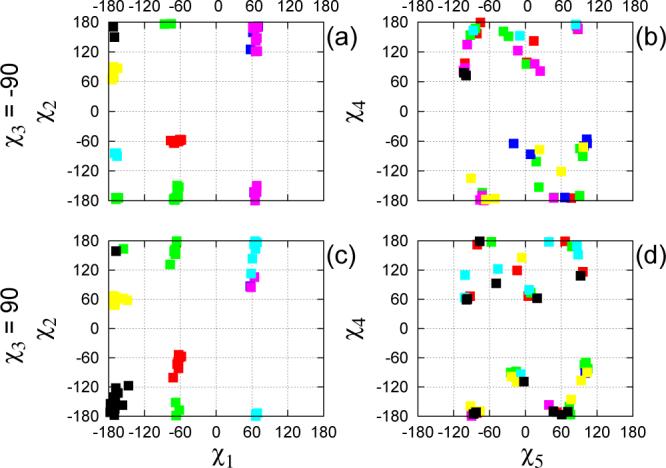
This relation is the dual of eq (37), since it expresses π in terms of $\tilde{\pi }$ and W = [w_ai]. The duality can be depicted as follows:

Starting from the quantities in one of the ellipses the quantities in the other ellipse are obtained using the specified equations.

In refs ³² and ⁴¹, following the top arrow to go from π to $\tilde{\pi }$ was called restriction, whereas going in the opposite direction was called interpolation. According to this nomenclature, H and W are the operators of restriction and interpolation. The former “restricts” any probability density over the microstates to a probability density over the macrostates (eq (35)), whereas the latter “interpolates” a detailed probability density from a coarse-grained one as

$$p\left(t\right)=\tilde{p}\left(t\right)W.$$ (41)

This naive way of building detail is based on the assumption that the internal probability structure of a macrostate is always in equilibrium. Note that, in general, restriction (eq (35)) followed by interpolation (eq (41)) does not recover the starting microstate probability vector:

$$p\left(t\right)\ne p\left(t\right)HW=p\left(t\right)A.$$ (42)

The last equality defines the stochastic matrix A. Only the microstate equilibrium probability is invariant under this operation, π = πA. Since the action of A on an arbitrary vector leads to a probability vector that is automatically equilibrated inside each of the macrostates, A can be viewed as an operator of intra-macrostate equilibration.

In all the present variants of lumping the microstates into macrostates, a membership array H is sought, such that the macrostate TPM

$$\tilde{P}\left(\tau \right)=WP\left(\tau \right)H$$ (43)

captures the slow dynamics of the Markovian microstate propagation as best as possible. Various algorithms for constructing “sharp”^26,35 or “fuzzy”^34,36 H from a given P have been proposed. (Equation (43) reduces to the more familiar

$${\tilde{P}}_{ab}\left(\tau \right)=\frac{\sum _{i\in a}\sum _{j\in b}{\pi }_i{P}_{ij}\left(\tau \right)}{\sum _{i\in a}{\pi }_i},$$ (44)

when the elements of H are restricted to be only zero or one, i.e. macrostates are defined with sharp boundaries.) The lower dimensional matrices P̃(τ) are then used to propagate directly the macrostate probabilities in a Markovian fashion as

$$\tilde{p}\left(0\right)\stackrel{\tilde{P}\left(\tau \right)}{\to }\tilde{p}\left(\tau \right)\stackrel{\tilde{P}\left(\tau \right)}{\to }\tilde{p}\left(2\tau \right)\stackrel{\tilde{P}\left(\tau \right)}{\to }$$ (45)

As clearly demonstrated in refs ³² and ⁴¹, because of the noncommuting nature of propagation and restriction, the matrices P̃(τ) fail to generate Markovian dynamics in the space of the macrostates. The problem is that a two-step microstate propagation followed by lumping does not lead to the same probability density as a lumping followed by a two-step macrostate propagation. This is easily seen using matrix notation:

$$\tilde{P}\left(\tau \right)\tilde{P}\left(\tau \right)=WP\left(\tau \right)AP\left(\tau \right)H\ne WP\left(\tau \right)P\left(\tau \right)H=\tilde{P}\left(2\tau \right).$$ (46)

The implication is that estimating P̃(τ) using a given lag time and squaring it is systematically different from P̃(2τ) estimated with twice as long a lag time. From eq (46), it is clear that by squaring P̃(τ) it is assumed that between two time steps separated by τ the microstates inside a macrostate reach their local equilibrium (imposed by the matrix A). Thus, replacing the detailed microstate dynamics by coarse-grained macrostate propagation relies on the assumption that after a jump to a new macrostate, the chain dwells inside the macrostate long enough to sample its equilibrium distribution before exiting it. This is achieved to a large degree by grouping microstates that exchange fast into macrostates, which, on the other hand, are chosen to be as weakly coupled as possible. In spite of that, occasionally, short-lived visits into macrostates are possible. Their presence leads to an artificially faster macrostate dynamics and is the physical reason behind the inequality in eq (46). To distinguish such brief visits from “real” transitions, we analyze the time series of the order parameters with a hidden Markov model (HMM).

3. Using hidden Markov models

HHMs have found widespread application in areas as diverse as speech recognition,⁴² analysis of currents from single ion channels,^43,44 or other single molecule data.⁴⁵ In this section, we utilize the well-established methodology of HMMs⁴² as a framework that aims to identify state boundaries and interstate transitions probabilistically, by considering the data as a time-ordered sequence of events.

In a HMM, the states of the Markov chain are not directly observed. What is observed is the d-dimensional vector of order parameters O_t, which is modeled to be “emitted” when the chain is in state i according to some probability density. For analytical tractability, it is convenient to choose the probability density for observing O_t = y, when X_t = i, as a multivariate Gaussian with a mean vector μ_t and a covariance matrix ∑_i:

$$\begin{array}{cc}\hfill b_i\left(\mathit{y}\right)& =\mathbb{P}\{{\mathit{O}}_t=\mathit{y}\mid X_t=i\}\hfill \\ \hfill & \propto \sqrt{\frac{\det \left\{{\Sigma }_i^{-1}\right\}}{{\left(2\pi \right)}^d}}{\mathrm{e}}^{-\frac{1}{2}{(\mathit{y}-{\mu }_i)}^{\mathsf{T}}\cdot {\Sigma }_i^{-1}\cdot (\mathit{y}-{\mu }_i)},\hfill \end{array}$$ (47)

where ${\nu }^{\mathsf{T}}$ indicates the transpose of ν. Given the sequence of observations, O = O₁, O₂, . . . O_T , and the parameters of the HMM, θ = {p, P(τ), μ_t,∑_i}, it is possible⁴² to calculate the conditional probability

$${\xi }_{ij}\left(t\right)=\mathbb{P}\{X_t=i,X_{t+1}=j\mid O,\theta \}$$ (48)

for the chain to be in state i at time step t and state j at time step t + 1. This iterative procedure is presented in Appendix 2. (The ith entry of the probability vector p that appeared in θ corresponds to the probability of the chain to start in state i.) With the help of ξ_ij(t) it is straightforward to calculate the expectation

$$\mathbb{E}\{N_{ij}^{\tau }\mid O,\theta \}=\sum _{t=1}^{T-1}{\xi }_{ij}\left(t\right),$$ (49)

which can be used in eq (29) instead of $N_{ij}^{\tau }$ to estimate P(τ). To update the other parameters of the HMM it is convenient to consider the probability to be in state i at time t, given O and θ:⁴²

$${\gamma }_i\left(t\right)=\mathbb{P}\{X_t=i\mid O,\theta \}=\sum _{j=1}^N{\xi }_{ij}\left(t\right).$$ (50)

With it, the parameters are updated as follows:⁴²

$$p_i={\gamma }_i\left(1\right),P_{ij}\left(\tau \right)=\frac{\sum _{t=1}^{T-1}{\xi }_{ij}\left(t\right)}{\sum _{t=1}^{T-1}{\gamma }_i\left(t\right)}$$ (51)

and

$${\mu }_i^{\text{new}}={\mu }_i^{\text{old}}+{\stackrel{‒}{\mu }}_i,{\Sigma }_i^{\text{new}}={\stackrel{‒}{\Sigma }}_i-{\stackrel{‒}{\mu }}_i{\stackrel{‒}{\mu }}_i^{\mathsf{T}},$$ (52a)

where

$${\stackrel{‒}{\mu }}_i\equiv \frac{\sum _{t=1}^T{\gamma }_i\left(t\right)({\mathit{O}}_t-{\mu }_i^{\text{old}})}{\sum _{t=1}^T{\gamma }_i\left(t\right)}$$ (52b)

$${\stackrel{‒}{\Sigma }}_i\equiv \frac{\sum _{t=1}^T{\gamma }_i\left(t\right)({\mathit{O}}_t-{\mu }_i^{\text{old}}){({\mathit{O}}_t-{\mu }_i^{\text{old}})}^{\mathsf{T}}}{\sum _{t=1}^T{\gamma }_i\left(t\right)}.$$ (52c)

These equations can be derived using maximum likelihood arguments.^46,47 When the order parameters are angles, periodic boundary conditions need to be imposed on the difference $O_t-u_i^{\mathrm{old}}$.

The hidden Markov modeling strategy presented here shares similarities with the K-means clustering: in both of the methods the number of desired states (clusters) is provided as an input; for each cluster, a representative point (“centroid” in K-means, μ_t in the HMM) is determined and its members are assigned in an iterative way; the assignment of membership relies on the choice of a distance metric in the space of order parameters. Nevertheless, crucial differences separate the two methods. Clusters in the K-means clustering are identified by considering only the geometric distances between the data points. Since information about the temporal ordering of the data is completely ignored, one can only hope that the resulting dynamics of jumping from cluster to cluster will turn out to be Markovian. States in the HMM strategy, on the other hand, are identified by using both the geometric distances and the temporal ordering of the data, having in mind the expected Markovian dynamics. Needless to say, all those advantages come at the expense of increased computational effort, which, considering the resources demanded by the generation of the starting MD trajectories, is well justified.

The HMM analysis can be easily extended to the lumping step. To preserve the spatial resolution o ered by the microstates, we retain the number of Gaussian basis functions using the same microstate emission probability densities as before (eq (47)). We look for M macrostates with Markovian dynamics according to some probability matrix P̃(τ). No dynamics are associated with the microstates. The emission probability b_a from each macrostate a, is a mixture of the N microstate components b_i:

$$b_a\left(\mathit{y}\right)=\sum _{i=1}^N{w}_{ai}{b}_i\left(\mathit{y}\right),1\le a\le M,$$ (53)

where w_ai is the probability contribution of i to a (eq (38)). Thus, we deal with a HMM in which the emission from each (hidden) macrostate is a mixture of Gaussian components. The iterative calculation of γ_a(t) (eq (50)) and the update of the starting probabilities and the transition matrix (eq (51)) remain unchanged, with the understanding that now the indices stand for macrostates. For the estimation of the microstate properties it is useful to introduce⁴²

$${\gamma }_{ai}\left(t\right)={\gamma }_a\left(t\right)\frac{w_{ai}{b}_i\left({\mathit{O}}_t\right)}{b_a\left({\mathit{O}}_t\right)}\text{and}{\gamma }_i\left(t\right)=\sum _{a=1}^M{\gamma }_{ai}\left(t\right).$$ (54)

The former is the probability of being in macrostate a at time step t having generated O_t from microstate i. The latter is the probability of emitting O_t at time t from a microstate i, idependently of what the macrostate is. The contributions of the microstates to the macrostates are updated as

$$w_{ai}=\frac{\sum _{t=1}^T{\gamma }_{ai}\left(t\right)}{\sum _{t=1}^T{\gamma }_a\left(t\right)},$$ (55)

whereas μ_t and ∑_i are calculated from eqs (52).

III. RESULTS

The methodology presented above is applied to a set of 18 MD trajectories of a spin labeled, 15-residue, poly-alanine α-helix. Details about those simulation were provided previously in paper I, and are only outlined in the following. The system was fully solvated with 686 TIP3P waters and simulated using the CHARMM program.⁴⁸ The resulting system of of 2247 atoms filled a tetragonal simulation box with starting side lengths of 26.0, 26.0 and 34.0 Å. Periodic boundary conditions were used. The electrostatics were treated with particle mesh Ewald summation.^49,50 Pressure and temperature pistons were used to achieve an NpT ensemble at T = 297 K and p = 1 atm.⁵¹ To prevent the unfolding of the helix in water the first five and the last five residues were harmonically restrained to their starting positions with force constants of 0.5 kcal/mol/Ų. Each of the 18 trajectories extended for 100 ns. Snapshots were saved every 1 ps. All additional details about the simulations can be found in paper I.¹

A. Building the Markov chain models

The analysis of the conformational dynamics of R1 at a poly-alanine α-helix, presented in paper I, suggests that the five dihedrals of the spin label represent a good set of order parameters to monitor its dynamics. An alternative set of order parameters, that has been used frequently to simulate the dynamics of spin labels and calculate ESR spectra,^52–54 are the Euler angles Ω_MN that parametrize the transformation of the helix-fixed coordinate system M to the nitroxide-fixed system of axes N. To compare these two choices, we attempted the construction of two Markov chain models: one, using the spin label dihedral angles, and the other, using the Euler angles. The MD snapshots from each of the 18 trajectories were first projected to the space of the order parameters. The resulting points in five or three dimensions were then clustered using the K-means algorithm.³³ The latter is based on the definition of distance in the multidimensional space of the order parameters. We chose an Euclidian distance metric in the five dimensional space of the dihedral angles. The only complication, related to the periodicity of the angles, was treated by restricting the separation between two points in each of the dimensions to be always in the range (−180°, 180°). Since selecting a distance metric in the space of the Euler angles is not trivial, we chose to work with quaternions of unit length. Such quaternions live on the surface of a four-dimensional unit sphere for which the great circle arc between two points defines a natural distance metric.^55,56

Considering the multiplicity of its five linker dihedral angles (χ₁ : 3, χ₂ : 3, χ₃ : 2, χ₄ : 3, and χ₅ : 2) the spin label R1 potentially has 108 rotamers. To ensure the complete coverage of all the rotamers, the K-means clustering algorithm was initiated with 120 clusters. For the model using the dihedral angles as order parameters, 108 centroids were initialized at the ideal, “reference” dihedral angles of each rotamer (±60°, 180° for multiplicity of 3, ±90° for multiplicity 2). The remaining 12 centroids were chosen randomly by generating random numbers from a uniform distribution in the angular range (−180°, 180°). For the other model, the initial 120 centroids were chosen to be uniformly-distributed random unit quaternions.⁵⁶ When the dihedral angles were used to build the centroids, some of the initial centroids failed to have any snapshots assigned to them. Such centroids were moved around randomly before the next iteration. This was repeated until all the 120 centroids acquired members. For the two choices of order parameters, convergence was assumed when the average centroid shift in one iteration was less than 10⁻⁵ degrees in the space of the five dihedral angles, and less than 10⁻⁴ on the surface of the four-dimensional unit sphere.

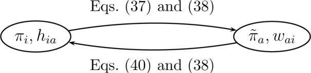
As a result of the clustering, the trajectories of the order parameters were converted to time series of jumps between 120 discrete states. These were then used to construct TPMs for values of τ ranging from 50 to 800 ps. The time scales τ_i, implied by the nonnegative eigenvalues of P(τ), were calculated from eq (31). The slowest 22 time scales are shown in Figure 1 as a function of τ for the two models. The independence of the relaxation times on the lag time is a signature of a good Markovian model. Whereas the lines are more or less horizontal in Figure 1a, they are significantly sloped in Figure 1b. More importantly, according to the first model, the slowest dynamical event occurs on a time scale of ∼70 ns, followed by two other events on time scales ∼10 ns; these time scales are completely missing in the second model.

Figure 1.

Time scales τ_i (1 ≤ i ≤ 22) of the two K-means-based Markov models as a function of lag time τ: (a) dihedral angles and (b) quaternions (Euler angles) used as order parameters.

From the analysis of the internal dynamics of R1 reported in paper I, we know that the rarest dynamical event in this system is the transition of the disulfide torsion angle χ₃ between its two energetically preferred values of ±90°. The additional analysis, presented below, confirms that the slowest relaxation time in Figure 1a is associated with the flip of χ₃. The absence of a similar slow time scale in Figure 1b indicates that the information regarding the state of χ₃ is lost when the conformation of R1 is projected to the space of the Euler angles. Based on this observation, we conclude that the Euler angles do not constitute good order parameters for reporting the dynamics of R1 on a poly-alanine α-helix, and do not consider them further.

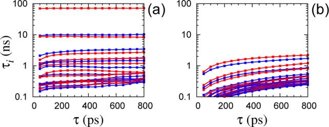
In Figure 1a, the time scales τ_i show relatively little dependence on the lag time τ, indicating that the jump dynamics among the K-means clusters are approximately Markovian. Nevertheless, when plotted on a linear scale, some of the τ_i < 5 ns are seen to rise throughout the whole examined range of τ without reaching a plateau (Figure 2a). A context dependent analysis is expected to alleviate this problem. A HMM with 120 microstates was constructed analyzing the time series of the five dihedral angles with a lag time τ = 100 ps. The probability densities for observing a certain combination of the torsion angles, given the state of the Markov chain, were chosen as in eq (47). The initial estimates of μ_t were taken to coincide with the positions of the K-means centroids, determined in the previous step. The starting covariance matrices ∑_i were also calculated according to the membership assigned by the K-means clustering. The parameters of the HMM were optimized using eqs (51) and (52). At the end of each iteration, microstates with less than 100 snapshots assigned to them, were removed. Convergence was assumed when each of the entries of the TPM changed by less than 10⁻³ in an iteration. After convergence, the Viterbi algorithm⁴² was used to generate time series of the hidden states, which were then used to estimate TPMs for integer multiples of the lag time used in the optimization. The time scales τ_i < 5 ns, of the obtained TPMs are shown in Figure 2b. Comparison with the same time scales estimated directly from the K-means clustered trajectories (Figure 2a) reveals that the time scales determined from the HMM are less dependent on τ and attain their asymptotic values at much shorter lag times.

Figure 2.

Time scales τ_i (4 ≤ i ≤ 22) of the transition matrices P(τ) estimated from the time series produced by (a) the K-means clustering and (b) the Viterbi algorithm after a HMM optimization with τ = 100 ps. The five linker dihedral angles were used as order parameters.

In Table I, we compare the slowest 14 time scales τ_i, calculated using P(τ), determined at τ = 100 ps, either (i) directly by the HMM optimization (P), or (ii) from the microstate trajectories generated with the Viterbi algorithm (traj.). For all practical purposes, the two alternatives appear to be basically identical. The presence of gaps between the relaxation time scales τ_i implies the existence of relatively weakly coupled sub-blocks in the Markov chain.^30,34,36 From the gaps in Figures 1a and 2b, it is clear that the conformational dynamics of R1 can be understood as a hierarchy of Markov chains with 2, 4, 6, 14, etc. number of macrostates. Which one of those chains to choose depends on the desired temporal resolution.

TABLE I.

The time scales τ_i (ns), for models with 120, 6 and 14 states, calculated using τ = 100 ps.

	N = 120		M = 6		M = 14
i	traj.	P	sharp	P̃	sharp	P̃
1	70.8	70.8	67.8	70.1	68.5	70.4
2	10.8	10.8	8.29	9.60	8.50	10.0
3	8.85	8.81	7.90	8.23	8.14	8.46
4	3.32	3.26	1.67	3.10	2.19	3.78
5	2.58	2.55	1.12	2.14	1.40	2.86
6	1.76	1.74	-	-	1.22	1.78
7	1.68	1.66	-	-	1.00	1.72
8	1.37	1.37	-	-	0.89	1.36
9	1.15	1.14	-	-	0.88	1.21
10	1.11	1.10	-	-	0.84	0.99
11	0.93	0.92	-	-	0.59	0.59
12	0.58	0.57	-	-	0.27	0.54
13	0.54	0.53	-	-	0.26	0.51
14	0.34	0.34	-	-	-	-

Markov models with M = 6, 14, 23, and 27 macrostates were constructed. During the optimization, the microstate properties μ_t and _i, were fixed and not allowed to change. The weights w_ai, with which microstate i contributes to the macrostate a, were optimized using the iterative procedure presented in Section II B 3. Convergence was assumed when each of the entries of the estimated TPM changed by less than 10⁻⁴ in an iteration. The required initial weights were assigned according to the lumping method of ref 35, which is extremely simple from a computational point of view. It groups microstates together in a macrostates using sharp membership. w_ai was intialized to 1 if a microstate i belonged to a macrostate a, and to 0.01 if it did not. These starting weights were normalized to satisfy eq (39).

The time scales of the macrostate TPMs determined after the convergence of the HMM procedure are shown in Table I for the first two models (P̃). In addition, the time scales of the transition matrices calculated from eq (44) from the sharp clustering of ref 35 are also shown (sharp). Since this clustering was used to initialize the weights w_ai, the difference between the two sets of time scales is an indicator of the improvement o ered by the HMM versus the lumping with sharp membership. For both M = 6 and M = 14 the improvement is seen to be significant, allowing the models to faithfully capture the slow dynamics of the detailed N = 120 model.

B. Analysis of the conformations

The hierarchical emergence of Markov models with 2, 4 and 6 states is followed in Table II. As expected, the division of states in the 2-state model is based on the value of χ₃. The populations of the χ₃ ≈ −90° and χ₃ ≈ +90° macrostates are estimated to be 88 % and 12 %, respectively (last row of Table I). The time scale associated with the flip of the disulfide dihedral is determined to be τ₁ ∼ 70 ns. This is the slowest event in the internal dynamics of the spin label R1, when it is situated at the middle of a poly-alanine α-helix. Since this time scale is expected to be largely determined by the dihedral energy barrier of χ₃ (about 7 kcal/mol)², the slow rate of exchange between the two conformations of the disulfide torsion angle is most likely a general characteristic of R1 at solvent-exposed sites in proteins. In the 4-state model, each of the χ₃ ≈ ±90° states is itself split in two: states with χ₁ ≈ 60° separate from the others. Such conformations place the S_γ of the spin label side chain in a sterically unfavorable position against the backbone atoms of the α-helix. According to the 6-state model, the populations of these states are barely a few percent (Table II), in agreement with the data for cysteine side chains on α-helices, for which χ₁ ≈ 60° is seen only 5% of the time.⁵⁷ These conformations of R1 are expected to be poorly populated at solvent-exposed sites in α-helices. The time scales τ₁ (∼ 70 ns), and τ₂, τ₃ (∼ 10 ns) indicate that the populations of the two χ₃ conformers and of the χ₁ ≈ 60° conformations, as well as the rates of their exchange, will be among the hardest to sample reliably in atomistic MD simulations. Certainly, for R1 at a general solvent-exposed site, there could be additional conformations which might be equally hard to sample. The remaining time scales of the internal R1 dynamics, according to the Markov models, are faster than 4 ns. From Table II, the slowest two of them (τ₄ ≈ 3.5 and τ₅ ≈ 2.5 ns) appear to be related to conformations with χ₂ ≈ 180° and χ₃ ≈ −90°.

TABLE II.

The characterization of the Markov models with 2, 4 and 6 states in terms of the dihedral angle conformations. The lifetimes of the states, from eq (32), are in bold.

2:	χ3	−90° (88.1%)				+90° (11.9%)
4:	χ1	−60°, 180°			+60°	−60°, 180°	+60°
	χ2	180°		−60°, +60°
6:		Ia	II	III	IV	V	VI
νa (ns)		2.4	6.1	5.2	9.8	55	8.7
${\tilde{\pi }}_a$ (%)		6.0	43.6	37.0	1.5	11.4	0.5

^aThis macrostate contains two microstates (the two black points in Figures 3a and 3b), which have very similar values for all the five dihedrals, μ_i ≈ (−170°, 160°, −95°, 75°, −100°).

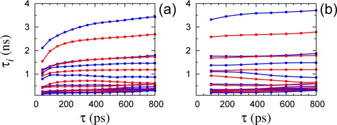
In Table III we show the populations of the 14-state model. To facilitate the presentation, the probabilites of the macrostates have been renormalized based on the χ₃ conformation to which they belong. The projection of the centroids μ_t, to the χ₁–χ₂ and χ₅–χ₄ planes, for microstates whose membership to a given macrostate is larger than 0.8, are shown in Figure 3. The microstates in a given macrostate are much more similar in terms of their χ₁ and χ₂ dihedrals, than in terms of χ₄ and χ₅. Even though localized, the projections of the macrostates on the χ₁–χ₂ plane are somewhat irregular, and, especially in the χ₂ direction, extend well beyond the ideal positions (±60° and 180°) expected for a torsion angle with multiplicity of 3. A few microstate centroids have χ₂ ≈ ±120°, which would constitute barriers for the ideal dihedral. In Figure 4 we show the R1 conformations corresponding to some of the μ_t's from Figure 3. The major source of intra-macrostate disorder is seen to be related to the last two dihedrals of the spin label side chain. At the same time, one of the shown microstates in macrostate 2 has a different χ₁ value from the others. Since the 14-state model lumps together conformations with exchange time faster than half a nanosecond (τ₁₃ ≈ 0.5 ns in Table I), this indicates that it is possible to have rather fast flips of χ₁. The TPMs of the 6- and 14-state models are shown in Figure 5. The states on the left-hand side correspond to χ₃ ≈ −90°, those on the right-hand side to χ₃ ≈ 90°. Bidirectional transitions between the two sets of conformations involve macrostates 2 and 9 (cf. Figure 4). A unidirectional transition is seen to connect macrostate 13 to 6. The states with χ₁ ≈ 60° are also observed to be connected to the others through one-way transitions. One-way transitions in the probability matrix are due to the limited sampling from the finite length MD trajectories.

TABLE III.

Populations (%) and lifetimes (ns) of the 14-state Markov model, normalized separately for conformations with χ₃ ≈ −90° (states 1 to 7), and χ₃ ≈ 90° (states 8 to 14). The states with χ₁ ≈ 60° are indicated with a star.

state #	1	2	3*	4*	5	6	7	tot.
popul.	26.8	49.0	0.9	0.8	6.8	9.3	6.4	100.0
lifetime	3.8	5.9	1.3	1.0	1.4	2.4	2.6
state #	8	9	10*	11*	12*	13	14	tot.
popul.	34.1	34.0	0.1	0.4	3.6	14.1	13.7	100.0
lifetime	2.4	1.3	1.1	0.7	3.6	1.7	0.8
colora	red	green	blue	purple	cyan	yellow	black

^aUsed in Figures 3 and 4.

Figure 3.

Positions of the 120 mean vectors μ_t projected to the χ₁–χ₂ and χ₅–χ₄ planes (colored according to the scheme in Table III).

Figure 4.

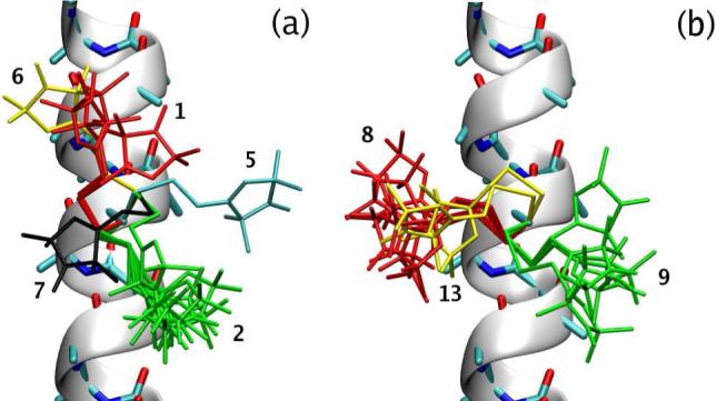
Spin label conformations corresponding to the microstate centroids μ_t which π_i > 1.2% and belong to macrostates with ${\tilde{\pi }}_a$ > 6.0% (according to the renormalized probabilities in Table III). The macrostates are numbered and colored following the convention of Table III. (a) χ₃ ≈ −90° conformations, (b) χ₃ ≈ −90°.

Figure 5.

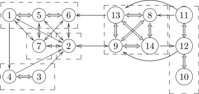
The hierarchical structure of the TPM for the 6-state (dashed boxes) and 14-state (circles) models. The correspondence between the states is as follows: I = {7}, II = {2}, III = {1, 5, 6}, IV = {3, 4}, V = {8, 9, 13, 14}, and VI = {10, 11, 12}. Intra-macrostate transitions for the 6-state model are indicated with block arrows and correspond to larger transition probabilities. The directions of the arrows indicate the directions of the transitions observed in the trajectories.

C. Multifrequency ESR spectra

Here we aim to compare spectra simulated using the stochastic jump trajectories according to the motional model

$$\mathrm{L}\stackrel{\begin{array}{c}\hfill \text{rotational}\hfill \\ \hfill \text{diffusion}\hfill \end{array}}{\to }\mathrm{M}\stackrel{\begin{array}{c}\hfill \text{Markov}\hfill \\ \hfill \text{chain}\hfill \end{array}}{\to }\mathrm{N}$$ (56)

with spectra simulated directly from the MD trajectories according to

$$\mathrm{L}\stackrel{\begin{array}{c}\hfill \text{rotational}\hfill \\ \hfill \text{diffusion}\hfill \end{array}}{\to }\mathrm{M}\stackrel{\begin{array}{c}\hfill \mathrm{MD}\hfill \\ \hfill \text{trajectories}\hfill \end{array}}{\to }\mathrm{N}.$$ (57)

In these diagrams, N is the coordinate system attached to the spin label, M is the coordinate frame attached to the helix, and L is the stationary lab-fixed frame. Rotational Brownian diffusion of M with respect to L, with diffusion coe cient D = 18 × 10⁶ s⁻¹, is introduced to represent the tumbling in solution of a small soluble protein like T4 Lysozyme. The dynamics of the spin label with respect to the helix is accounted for by the trajectories of either the Markov models or the MD simulations. One deficiency of the MD simulations, which is also propagated to the Markov models constructed from them, is related to the fact that the viscosity of the TIP3P water model used in the MD simulations is roughly 2.8 times smaller than the viscosity of water.^58,59 As a result, the motion of the solvent-exposed spin label is not su ciently damped down by the lack of viscous drag and the dynamical transitions occur on a timescale that is too fast. Addressing this problem thoroughly would require an extensive reparameterization of the force field, which goes beyond the scope of the present effort. However, to enable a qualitative assessment of the method, it is of interest to have the simulated dynamical transitions on timescales that approach those of the experiments. Following a simple argument valid for diffusive systems, in the calculation of ESR spectra, the time axis of both the MD simulations and the estimated Markov models was stretched by a factor of 2.5 to correct for the this faster solvent dynamics. One may expect this simple empirical scaling procedure to be qualitatively valid for solvent-exposed moieties. The details of the numerical propagation of the quantal dynamics and the stochastic rotational diffusion were given elsewhere.⁶⁰ Below we summarize the values of the various integration parameters.

When spectra were simulated for the model (57), the numerical propagation of the quantal spin dynamics and the rotational diffusion was carried with a time step Δt. The choice of the time step was based on the requirement that replacing a spin Hamiltonain varying over a time window Δt by an average Hamiltonian is formally justified. This condition leads to different values of Δt for different strengths of the magnetic field (Table IV).⁶⁰ Average magnetic tensors were calculated from the MD trajectories for successive time intervals of duration Δt. Since the MD snapshots were saved every 1 ps (= 2.5 ps after the stretch of the time axis), time-averaged magnetic tensors were calculated by averaging over ‘avgN’ successive snapshots (Table IV). Following paper I, the quantum integration was initialized at time intervals separated by 2 ns along each of the MD trajectories, which corresponds to ‘lagN’ number of Δt steps. The columns ‘sphN’ and $T_{\mathrm{L}}^{-1}$ in Table IV list, respectively, the number of spherical grid points used for the initial conditions of the isotropic diffusion, and the Lorentzian broadening introduced in the calculation of the spectra. The magnetic tensors were taken to be

$$\begin{array}{cc}\hfill {\mathrm{g}}^{\mathrm{N}}& =\text{diag}(2.00809,2.00585,2.00202)\hfill \\ \hfill {\mathrm{A}}^{\mathrm{N}}& =\text{diag}(6.2,4.3,36.9),\hfill \end{array}$$ (58)

in agreement with the values used in paper I.

TABLE IV.

Parameters used in the simulation of the ESR spectra from the MD and the Markov chain trajectories.

field (T)	Δt (ns)	avgN	lagN	sphN	TL−1 (G)	M
0.33	2.0	800	1	400a	0.8	14
3.40	0.5	200	4	3200b	1.2	23
6.09	0.4	160	5	6400b	2.2	27

^aTwice as many points were used with the Markov trajectories.

^bFour times more points were used with the Markov trajectories.

When spectra were simulated with the Markov model (56), the time intervals Δt of Table IV were used as indicators of the minimal temporal resolution the model was expected to provide. The (approximate) number of required macrostates, was determined by examining the eigenvalues of the N = 120 microstate model. Three such values, corresponding to time scales slower than, respectively, 0.8, 0.2 and 0.16 ns (after accounting for the 2.5 scaling of the time axis), are listed in the last column of Table IV. For all the models, trajectories were generated with the macrostate transition matrix P̃(τ) estimated at τ = 100 ps (= 250 ps after scaling by 2.5). This time step was used to integrate the stochastic dynamics model (56) (i.e. to generate the Markov jump and the rotational diffusion trajectories) and to propagate the quantum dynamics. Note that this time step is smaller than all the Δt's given in Table IV, and thus is appropriate for the simulation of ESR spectra for any of the three field strengths. 200 independent Markov jump trajectories were simulated per spherical grid point.

A direct comparison between the two motional models (57) and (56) is encumbered due to the differences in the relative populations of the states as determined from the MD trajectories and from the Markov model. The populations of the two χ₃ conformations, for example, are present in a 2:1 ratio in the MD trajectories, as discussed in paper I, whereas the 6-state model gives a ratio of 88:12 (Table II). The latter number takes into account not only the total time spent in each state (2:1), which for nonergodic trajectories is heavily determined by the initial conditions, but also the ratio of the number of observed p→m and m→p transitions (4:1). To circumvent this complication, we simulate and compare spectra for conformations with χ₃ ≈ −90° and 90° separately. Based on the time scales in Table I, we expect the sampling inside each of these two conformations to be approximately ergodic.

Recently, multifrequency spectra at 9.5, 95 and 170 GHz (0.33, 3.4 and 6.09 T) have been reported for R1 at position 131 in T4 Lysozyme.⁶¹ Motivated by this study, we compare spectra simulated using the Markov state trajectories and the MD trajectories for the three field strengths (Figure 6). Spectra from models with number of states estimated to be su cient for a given field strength (column M in Table IV) lie along the diagonal running from the upper left corner to the lower right corner of Figure 6. These are seen to be essentially identical to the spectra below the diagonal for all the three field strengths, indicating convergence with respect to the number of Markov states. In comparison, the spectra above the diagonal (from models with less states than necessary) exhibit sharper features. The presence of such sharp features is a well known effect in simulations based on average Hamiltonians (also called effective Hamiltonian).^62,63 For all fields, the agreement between the spectra simulated using the MD and the Markov trajectories is rather good for the χ₃ ≈ −90° conformations (top spectra in each plot). The spectra of the χ₃ ≈ 90° conformations (at the bottom of each plot), on the other hand, show systematic differences: at all fields the spectra simulated using the Markov chain dynamics exhibit sharper features than the corresponding spectra simulated using the MD trajectories. This is an indication that modeling the dynamics of the χ₃ ≈ 90° conformers with the model (56) suffers from the “average Hamiltonian” effect.

Figure 6.

Comparison of multifrequency spectra simulated directly using the MD trajectories (black lines) and the stochastic trajectories generated using M-state Markov models (colored lines). Spectra simulated from the χ₃ ≈ −90° and χ₃ ≈ 90° sub-blocks of the full transition probability matrix are shown at the top (blue) and bottom (red) of each plot.

IV. DISCUSSION

A systematic method for constructing Markov chain models from the MD trajectories of the side chain R1, using the values of its dihedral angles as order parameters, was presented. Starting from numerous clusters, determined by the K-means clustering algorithm, we gradually proceeded to construct Markov models with reduced number of states. At every stage we formulated the problem as an inference of a HMM, and relied on the probabilistic framework developed for such models.⁴² The states of the constructed Markov models were examined to gain an insight into the metastable conformations of R1 on a poly-alanine α-helix. Stochastic trajectories were generated using the estimated TPMs, and used to simulate ESR spectra at three different field strengths.

The motivation to use HMMs came from the work of Horenko et al.,^64–66 in which a HMM with overdamped, diffusive dynamics inside each of the hidden states was developed. As mentioned before, a TPM estimated by pure counting (according to eq (29)) exhibits apparent memory at short lag times, which results from counting short-lived excursions across macrostate boundaries as genuine transitions. This effect is significantly reduced if such excursions are identified, and treated accordingly by using a HMM, as demonstrated in the context of R1 on a poly-alanine α-helix (Figure 2). Certainly, the extent to which sharp macrostate boundaries and their fast recrossings are a problem, depends on the time scale separation between the intra-macrostate equilibration and inter-macrostate dynamics.

A. Euler angles

In a number of previous studies, MD trajectories of R1 have been used to construct stochastic models of its dynamics by relying on the Euler angles Ω to report on the orientation of the nitroxide-fixed frame N with respect to the macromolecular frame M.^52–54 In this approach, the MD trajectories are first used to estimate the potential of mean force U(Ω), then, diffusive Brownian dynamics (BD) trajectories propagated on U(Ω) are used to calculate ESR spectra. In refs ⁵² and ⁵³ and U(Ω) was calculated by partioning the Euler angle space into bins of width 3.6° along each of the three angles and estimating the probability histogram from the MD snapshots. In ref 54, U(Ω) was assumed to depend only on two out of the three Euler angles, which allowed for its expansion in terms of spherical harmonics.

The unrealistically fast dynamics in Figure 1b, when compared with Figure 1a, indicates that by monitoring only the values of the Euler angles, one is insensitive (“blind”) to the state of the disulfide torsion angle χ₃. When the regions of accessible to the two conformations of χ₃ overlap, an algorithm in which the propagation is based solely on the current values of the Euler angles is unable to recognize this process as a rare transition. In such cases, it is not legitimate to build a memoryless BD model based on a single effective energy surface U(Ω) since the true dynamics depend on additional degrees of freedom which are not explicitly accounted for. It is possible that for restricted spin labels, for which certain values of Ω are accessible only from unique structural conformations, the dynamics projected onto the Euler angles could provide a faithful representation of the internal spin label dynamics. For R1 at solvent-exposed helix surface sites, however, our results suggest that the Euler angles are not good order parameters to characterize its internal dynamics. From that perspective, the potential of mean force U(Ω), even though accessible computationally, is largely irrelevant for the dynamics of R1 at such sites.

B. Rotameric dynamics of R1

In Figure 4 we saw that the inter-macrostate disorder was mainly due to variation in the values of the last two dihedrals χ₄ and χ₅. At first glance, this might look as a support of the χ₄/χ₅ model, proposed to rationalize the internal dynamics of R1 relevant for the ESR spectra.^63,67 According to the model, the transitions of χ₁, χ₂ and χ₃ are too slow to be dynamically relevant for the ESR spectra. Thus, the deviation of the spectral line shape from the rigid limit is mainly due to transitions of χ₄ and χ₅. The time scales presented in Table I, and the characterization of the states in Table II, suggest that only the time scale associated with the χ₃ transition falls in the rigid limit, whereas all the others are on the order of 10 ns or faster. Hence, the segmental motion of all the dihedrals, except χ₃, has the potential to contribute to the deviation of the spectrum away from the rigid limit.

The Markov chain analysis of the R1 conformations and their time scales of mixing identified the exchange between the states with different values of χ₃ and the populations of the states with χ₁ ≈ 60° as the hardest to sample reliably in free MD simulations. (Additional slow events are not ruled-out for R1 at solvent-exposed sites in proteins.) In spite of the sampling problem that these events pose, they do not hinder the simulation of ESR spectra. As already pointed out in paper I, due to the rather slow exchange rate of the two χ₃ conformers, the decay of the magnetization from each of them can be added linearly to obtain a spectrum for all frequencies including, and beyond, 9 GHz. Thus, their relative populations can be left as a free parameter of mixing and determined by fitting the simulated spectrum to an experimental one. In addition, even though the exact populations of the χ₁ ≈ 60° conformations and their rates of exchange might be largely uncertain, their influence on the spectra is probably insignificant because the populations are expected to be rather small in absolute terms for R1 at solvent-exposed sites on α-helices.

C. Average Hamiltonian

In the simulation of the ESR spectra only the average values of the magnetic tensors in a given macrostate were used, based on the result of Section II A summarized by eq (26). This equation is valid to zeroth order in the expansion parameter ε. Another term, proportional to the integral of the correlation function of the Liouvillian—the famous relaxation operator in the Redfield theory of relaxation—appears when the analysis is carried to higher order.^68,69 In ref 70, for example, the relaxation operator was calculated assuming overdamped torsional oscillations of R1. In principle, this term can also be included in the time domain propagation of the spin dynamics performed in this paper. There is a significant difference, though, between the average Liouvillian in eq (26) and the relaxation operator. Whereas the former corresponds to an average Hamiltonian in the Hilbert space of the problem, the latter necessitates the quantal propagation to be carried in Liouville space. As we have previously demonstrated,⁶⁰ propagating the density matrix in the Hilbert space is advantageous from a computational point of view. Therefore, to avoid using the relaxation operator, we introduce a large number of macrostates to insure that dynamics on the fast time scales is explicitly accounted for.

The multifrequency spectra of the χ₃ ≈ −90° conformations of R1 in Figure 6 demonstrate that the proposed strategy can perform perfectly well. The χ₃ ≈ 90° spectra, on the other hand, indicate that the temporal resolution provided by the 27-state Markov model (down to about 160 ps) is not su cient to resolve the relevant dynamics of those conformations of R1. At the same time, it is not advisable to increase the number of macrostates in the model, since for time scales faster than τ ≈ 100 ps a Markov model of the dynamics is seen not to be appropriate (Figure 2). The spectral line shapes in Figure 6 and the analysis of paper I indicate that the R1 conformations with χ₃ ≈ 90° are more disordered and mobile than the χ₃ ≈ −90° conformers. Spin labels located at the surfaces of proteins are expected to be more immobilized than the spin label of the present study due to the larger protein surface accessible for specific and/or nonspecific interactions. The formalism developed in this paper is therefore applicable to such spin labels.

V. CONCLUSION

Markov chain models constructed from MD trajectories of the spin label dynamics hold the potential of bridging the gap between atomistic MD simulations of solvated spin labeled proteins and their experimental ESR spectra. They provide a rigorous probabilistic framework for utilizing the information from many, independent MD trajectories toward a single, coherent model of the spin label dynamics. Not using the MD trajectories directly for the simulation of the spectra, removes the burden imposed by the slow decay of the transverse magnetization on the duration of a single dynamical trajectory. Using the MD trajectories to estimate conditional transition probabilities, makes it possible to use many (tens or hundreds), relatively short (tens of nanoseconds) simulations. Calculating realistic ESR spectra in quantitative agreement with experiment from atomistic MD simulations of a spin labeled protein, is therefore expected to become feasible in the near future. The framework developed in this paper is being applied to the dynamics of R1 at solvent-exposed sites in T4 Lysozyme.⁷¹ The current strategy has culminated in excellent agreement with multifrequency ESR experiments for the very first time.⁷²

APPENDIX: IMPLEMENTATION DETAILS

1. How to impose detailed balance

When a TPM is estimated directly from the time series using eq (29) it can have negative or/and complex eigenvalues. The presence of complex eigenvalues is a sign that P is not in detailed balance with its left eigenvector π. A legitimate TPM, in detailed balance with its equilibrium probability vector, can be constructed from any symmetric matrix with nonnegative entries. Let S be such a matrix and

$$s_i\equiv \sum _j{S}_{ij}$$ (A.1)

are its row sums. Then,

$$P_{ij}=\frac{S_{ij}}{s_i}\text{and}{\pi }_i=\frac{s_i}{\sum _i{s}_i}$$ (A.2)

are in detailed balance. This observation forms the basis of two different strategies for imposing detailed balance on transition matrices estimated from the data. In the first one, the available MD trajectories are analyzed both forward and backward in time, thus counting a forward j → i transition also as a backward i → j transition. With this understanding, the forward-backward (↔) transition count matrix becomes

$${\overleftrightarrow{N}}_{ij}^{\tau }=(N_{ij}^{\tau }+N_{ji}^{\tau })∕2,$$ (A.3)

which is symmetric by construction. Therefore, the matrix $\overleftrightarrow{P}\left(\tau \right)$ built from it by row normalization is automatically in detailed balance with its equilibrium eigenvector $\overleftrightarrow{\pi }$. In the second alternative,²³ P(τ) is built from the forward counts only according to eq (29). Then, its stationary eigenvector π is calculated. Since the forward transition count matrix is not necessarily symmetric, P(τ) and π need not be in detailed balance. They are used to build the symmetric matrix

$$S_{ij}=({\pi }_i{P}_{ij}+{\pi }_j{P}_{ji})∕2,$$ (A.4)

from whcih new $\overrightarrow{P}\left(\tau \right)$ and $\overrightarrow{\pi }$, in detailed balance with each other, are formed according to eq (A.2)

In each of these two ways the information present in the transition count matrix is utilized in a qualitatively different fashion. For concreteness, let us consider a two-state Markov model. Suppose that the simulated trajectories of the model result in

$$N^{\tau }=\left(\begin{array}{cc}\hfill 200\hfill & \hfill 5\hfill \\ \hfill 3\hfill & \hfill 800\hfill \end{array}\right),$$ (A.5)

for some lag time τ. This means that the total time spent in the states is 200 and 800 stpes, respectively. Also, the trajectories contain five 1 → 2 and three 2 → 1 transitions. Following the first procedure, we build the forward-backward count matrix

$${\overleftrightarrow{N}}^{\tau }=\left(\begin{array}{cc}\hfill 200\hfill & \hfill 4\hfill \\ \hfill 4\hfill & \hfill 800\hfill \end{array}\right),$$ (A.6)

for whcih ${\overleftrightarrow{P}}_{12}\approx 4∕200$ and ${\overleftrightarrow{P}}_{21}\approx 4∕800$. The equilibrium probabilities for the two states follow from the detailed balance condition, eq (30). For their ratio one finds

$${\overleftrightarrow{\pi }}_1∕{\overleftrightarrow{\pi }}_2={\overleftrightarrow{P}}_{21}∕{\overleftrightarrow{P}}_{12}\approx \frac{4∕800}{4∕200}=1∕4.$$ (A.7)

In the second case, ${\overrightarrow{P}}_{12}\approx 5∕200$ and ${\overrightarrow{P}}_{21}\approx 3∕800$. The detailed balance condition gives

$${\overrightarrow{\pi }}_1∕{\overrightarrow{\pi }}_2={\overrightarrow{P}}_{21}∕{\overrightarrow{P}}_{12}\approx \frac{3∕800}{5∕200}=3∕20,$$ (A.8)

which agrees with what is obtained from constructing

$$S=\left(\begin{array}{cc}\hfill 120\hfill & \hfill 3\hfill \\ \hfill 3\hfill & \hfill 800\hfill \end{array}\right)$$ (A.9)

using eq (A.4), and calculating $\overrightarrow{\pi }$ from eq (A.2). Clearly, the two ways of imposing detailed balance lead to drastically different equilibrium probabilities.

More careful examination of the two procedures reveals the source of the difference. Symmetrizing N^τ according to eq (A.3) makes sure that the number of i → j and j → i transitions are the same, without changing the diagonal terms. Since the number of transitions typically is much smaller than the numbers along the diagonal, such symmetrization basically implies that the ratio of the equilibrium probabilities will be dominated by the ratio of the diagonal elements, as was the case in eq (A.7). The ratio of the diagonal terms simply reflects the frequencies of observing the chain in each of its states over all of the available trajectories. For nonergodic trajectories, these frequencies do not correspond to the thermodinamic Boltzmann weights of the states, but are dominated by the state in which the trajectories were started. When only forward transitions are counted, the number of i → j and j → i transitions are not necessarily equal. In this case, the ratio of the equilibrium probabilities implied by the TPM depends not only on the ratio of the diagonal terms but also on the ratio of the observed transitions, as seen in eq (A.8). From this example it becomes clear that the forward-backward counting scheme of eq (A.3) presupposes that the available trajectories are ergodic and visit the states of the chain according to the equilibrium probabilities. When only relatively short trajectories are available, which is the situation that we deal with, the forward-only counting scheme uses the scarce but valuable information present in the o diagonal elements of N^τ together with the total times spent in each state (the diagonal elements) to estimate a more meaningful equilibrium probability vector.

2. Details about the HMM estimation

Let

$$O_{t:s}={\mathit{O}}_t,{\mathit{O}}_{t+1},\dots {\mathit{O}}_{s-1},{\mathit{O}}_s,1\le t<s\le T,$$ (A.10)

denote the sequence of observations from time step t to time step s, and O = O_1:T indicate the entire sequence of observations. The forward variables

$${\alpha }_i\left(t\right)=\mathbb{P}\{X_t=i,O_{1:t}\mid \theta \}$$ (A.11)

correspond to the conditional probability of observing the sequence of observations up to time t and being in state i at time t, given the parameters of the model. They can be calculated e ciently as

$$\begin{array}{cc}\hfill {\alpha }_i\left(1\right)& =p_i{b}_i\left({\mathit{O}}_1\right)\hfill \\ \hfill {\alpha }_j\left(t\right)& =\sum _{i=1}^N{\alpha }_i(t-1)P_{ij}{b}_j\left({\mathit{O}}_t\right),1<t\le T.\hfill \end{array}$$ (A.12)

The backward variables

$${\beta }_i\left(t\right)=\mathbb{P}\{O_{t+1:T}\mid X_t=i,\theta \},$$ (A.13)

are the conditional probabilities of observing the sequence O_t+1:T, given the parameters of the model and that the (hidden) state at time t is i. They can also be calculated recursively as

$$\begin{array}{cc}\hfill {\beta }_i\left(T\right)& =1\hfill \\ \hfill {\beta }_i\left(t\right)& =\sum _{j=1}^N{P}_{ij}{b}_j\left({\mathit{O}}_{t+1}\right){\beta }_j(t+1),T>t\ge 1.\hfill \end{array}$$ (A.14)

Once the forward and backward variables are known it is easy to calculate the conditional probability of observing the whole sequence of observations O, given the parameters of the model:

$$\mathbb{P}\{O\mid \theta \}=\sum _{i=1}^N{\alpha }_i\left(T\right)=\sum _{i=1}^N{\alpha }_i\left(t\right){\beta }_i\left(t\right).$$ (A.15)

The last equality holds for any 1 ≤ t ≤ T . Also, γ_i(t) and ξ_ij(t), defined in eqs (50) and (48), respectively, can be calculated as

$${\gamma }_i\left(t\right)=\frac{{\alpha }_i\left(t\right){\beta }_i\left(t\right)}{\mathbb{P}\{O\mid \theta \}}.$$ (A.16)

and

$${\xi }_{ij}\left(t\right)=\frac{{\alpha }_i\left(t\right)P_{ij}{b}_j\left({\mathit{O}}_{t+1}\right){\beta }_j(t+1)}{\mathbb{P}\{O\mid \theta \}}.$$ (A.17)

Once the parameters of the model are optimized one can find the best state sequence X₁X₂ . . . X_T corresponding to the observation sequence O. This is achieved using the following three step procedure known as the Viterbi algorithm:⁴²

$$\{\begin{array}{c}{\delta }_i\left(1\right)=p_i{b}_i\left({\mathit{O}}_1\right)\hfill \\ {\psi }_i\left(1\right)=0\hfill \end{array}\phantom{\}}$$ (A.18a)

$$\{\begin{array}{cc}{\delta }_j\left(t\right)={\max }_i\left\{{\delta }_i(t-1)P_{ij}{b}_j\left({\mathit{O}}_t\right)\right\}\hfill & \hfill \\ {\psi }_j\left(t\right)={\mathrm{argmax}}_i\left({\delta }_i(t-1)P_{ij}\right\},\hfill & 1<t\le T\hfill \end{array}\phantom{\}}$$ (A.18b)

$$\{\begin{array}{cc}{X}_T={\mathrm{argmax}}_i\left\{{\delta }_i\left(T\right)\right\}\hfill & \hfill \\ X_t={\psi }_{X_{t+1}}(t+1),\hfill & T>t\ge 1.\hfill \end{array}\phantom{\}}$$ (A.18c)

References

- 1.Sezer D, Freed JH, Roux B. J. Phys. Chem. B. 2008 doi: 10.1021/jp801608v. in press. [DOI] [PMC free article] [PubMed] [Google Scholar]
- 2.Jiao D, Barfield M, Combarzia JE, Hruby VJ. J. Am. Chem. Soc. 1992;114:3639–3643. [Google Scholar]
- 3.Kubo R. Journal of the Physical Society of Japan, Supplement. 1969;26:1–5. [Google Scholar]
- 4.Kubo R. Advances in Chemical Physics. 1969;15:101–127. [Google Scholar]
- 5.Kubo R. Journal of the Physical Society of Japan. 1954;9:935–944. [Google Scholar]
- 6.Freed JH, Bruno GV, Polnaszek CF. J. Phys. Chem. 1971;75:3385. [Google Scholar]
- 7.Polnaszek CF, Bruno GV, Freed JH. J. Chem. Phys. 1973;58:3185–3199. [Google Scholar]
- 8.Abragam A. Principles of Nuclear Magnetism. Oxford University Press; 1961. [Google Scholar]
- 9.Ernst RR, Bodenhausen G, Wokaun A. Oxford University Press; 1987. Principles of Nuclear Magnetic Resonance in One and Two Dimensions. [Google Scholar]
- 10.Schneider DJ, Freed JH. Adv. Chem. Phys. 1989;73:387–527. [Google Scholar]
- 11.Norris JR. Markov Chains. Cambridge University Press; 1997. [Google Scholar]
- 12.Mukamel S. Principles of Nonlinear Optical Spectroscopy. Oxford University Press; 1995. [Google Scholar]
- 13.Risken H. Springer-Verlag; 1984. The Fokker-Planck Equation. [Google Scholar]
- 14.Polimeno A, Moro GJ, Freed JH. J. Chem. Phys. 1996;104:1090–1104. [Google Scholar]
- 15.Vanden-Eijnden E. Comm. Math. Sci. 2003;1:385–391. [Google Scholar]
- 16.E W, Liu D, Vanden-Eijnden E. Comm. Pure Appl. Math. 2005;53:1544–1585. [Google Scholar]
- 17.Givon D, Kupferman R, Stuart A. Nonlinearity. 2004;17:R55–R127. [Google Scholar]
- 18.Just W, Kantz H, Rodenbeck C, Helm M. J. Phys. A: Math. Gen. 2001;34:3199–3213. [Google Scholar]
- 19.Just W, Gelfert K, Baba N, Riegert A, Kantz H. J. Stat. Phys. 2003;112:277–292. [Google Scholar]
- 20.Swope WC, Pitera JW, Suits F. J. Phys. Chem. B. 2004;108:6571–6581. [Google Scholar]
- 21.Swope WC, Pitera JW, Suits F, Pitman M, Eleftheriou M, Fitch BG, Germain RS, Rayshubski A, Ward TJC, Zhestkov Y, Zhou R. J. Phys. Chem. B. 2004;108:6582–6594. [Google Scholar]
- 22.Singhal N, Snow CD, Pande VS. J. Chem. Phys. 2004;121:415–425. doi: 10.1063/1.1738647. [DOI] [PubMed] [Google Scholar]
- 23.Elmer SP, Park S, Pande VS. J. Chem. Phys. 2005;123:114902. doi: 10.1063/1.2001648. [DOI] [PubMed] [Google Scholar]
- 24.Singhal N, Pande VS. J. Chem. Phys. 2005;123:204909. doi: 10.1063/1.2116947. [DOI] [PubMed] [Google Scholar]
- 25.Park S, Pande VS. J. Chem. Phys. 2006;124:054118. doi: 10.1063/1.2166393. [DOI] [PubMed] [Google Scholar]
- 26.Chodera JD, Singhal N, Pande VS, Dill KA, Swope WC. J. Chem. Phys. 2007;126:155101. doi: 10.1063/1.2714538. [DOI] [PubMed] [Google Scholar]
- 27.Singhal Hinrichs N, Pande VS. J. Chem. Phys. 2007;126:244101. doi: 10.1063/1.2740261. [DOI] [PubMed] [Google Scholar]
- 28.Ma A, Dinner AR. J. Phys. Chem. B. 2005;109:6769–6779. doi: 10.1021/jp045546c. [DOI] [PubMed] [Google Scholar]
- 29.Schütte C, Fischer A, Huisinga W, Deuflhard P. J. Comp. Phys. 1999;151:146–168. [Google Scholar]
- 30.Deuflhard P, Huisinga W, Fischer A, Schütte C. Lin. Algebra Appl. 2000;315:39–59. [Google Scholar]
- 31.Noe F, Horenko I, Schütte C, Smith JC. J. Chem. Phys. 2007;126:155102. doi: 10.1063/1.2714539. [DOI] [PubMed] [Google Scholar]
- 32.Kube S, Weber M. J. Chem. Phys. 2007;126:024103. doi: 10.1063/1.2404953. [DOI] [PubMed] [Google Scholar]
- 33.Hartigan JA. Clustering Algorithms. John Wiley and Sons Inc.; 1975. [Google Scholar]
- 34.Deuflhard P, Weber M. Lin. Algebra Appl. 2005;398:161–184. [Google Scholar]
- 35.van Dongen S. Ph.D. thesis. University of Utrecht; 2000. [Google Scholar]
- 36.Fritzsche D, Mehrmann V, Szyld DB, Virnik E. An SVD approach to identifying meta-stable states of Markov chains. 2006. Technical Report 06−08−04.
- 37.Sriraman S, Kevrekidis IG, Hummer G. J. Phys. Chem. B. 2005;109:6479–6484. doi: 10.1021/jp046448u. [DOI] [PubMed] [Google Scholar]
- 38.Shalloway D. J. Chem. Phys. 1996;105:9986–10007. [Google Scholar]
- 39.Deuflhard P. From Molecular Dynamics to Conformational Dynamics in Drug Design. 2002. Technical Report.
- 40.Weber M. Improved Perron Cluster Analysis. 2003. Technical Report.
- 41.Kube S, Weber M. Coarse graining molecular kinetics. 2007. Technical Report. [DOI] [PubMed]
- 42.Rabiner LR. Proc. IEEE. 1989;77:257–286. [Google Scholar]
- 43.Qin F, Auerbach A, Sachs F. Biophys. J. 2000;79:1915–1927. doi: 10.1016/S0006-3495(00)76441-1. [DOI] [PMC free article] [PubMed] [Google Scholar]
- 44.Venkataramanan L, Sigworth FJ. Biophys. J. 2002;82:1930–1942. doi: 10.1016/S0006-3495(02)75542-2. [DOI] [PMC free article] [PubMed] [Google Scholar]
- 45.McKinney SA, Joo C, Ha T. Biophys. J. 2006;91:1941–1951. doi: 10.1529/biophysj.106.082487. [DOI] [PMC free article] [PubMed] [Google Scholar]
- 46.Liporace LA. IEEE Trans. Inform. Theory. 1982;IT-28:729–734. [Google Scholar]
- 47.Bilmes JA. A Gentle Tutorial of the EM Algorithm and its Application to Parameter Estimation for Gaussian Mixture and Hidden Markov Models. 1998. Technical Report.
- 48.Brooks BR, Bruccoleri RE, Olafson BD, States DJ, Swaminathan S, Karplus M. J. Comp. Chem. 1983;4:187–217. [Google Scholar]
- 49.Darden T, York D, Pedersen L. The Journal of Chemical Physics. 1993;98:10089–10092. [Google Scholar]
- 50.Essmann U, Perera L, Berkowitz ML, Darden T, Lee H, Pedersen LG. The Journal of Chemical Physics. 1995;103:8577–8593. [Google Scholar]
- 51.Lamoureux G, Roux B. The Journal of Chemical Physics. 2003;119:3025–3039. [Google Scholar]
- 52.Steinhoff H-J, Hubbell W. Biophys. J. 1996;71:2201–2212. doi: 10.1016/S0006-3495(96)79421-3. [DOI] [PMC free article] [PubMed] [Google Scholar]
- 53.Beier C, Steinhoff H-J. Biophys. J. 2006;91:2647–2664. doi: 10.1529/biophysj.105.080051. [DOI] [PMC free article] [PubMed] [Google Scholar]
- 54.Budil DE, Sale KL, Khairy KA, Fajer PG. J. Phys. Chem. A. 2006;110:3703–3713. doi: 10.1021/jp054738k. [DOI] [PubMed] [Google Scholar]
- 55.Shoemake K. Proc. of SIGGRAPH '85. 1985:245–254. [Google Scholar]
- 56.Kuffner JJ. Proc. IEEE Int'l Conf. on Robotics and Automation (ICRA 2004) 2004:1–6. [Google Scholar]
- 57.Lovell SC, Word JM, Richardson JS, Richardson DC. Proteins. 2000;40:389–408. [PubMed] [Google Scholar]
- 58.Feller SE, Pastor RW, Rojnuckarin A, Bogusz S, Brooks BR. J. Phys. Chem. 1996;100:17011–17020. [Google Scholar]
- 59.Yeh I-C, Hummer G. Biophys. J. 2004;86:681–689. doi: 10.1016/S0006-3495(04)74147-8. [DOI] [PMC free article] [PubMed] [Google Scholar]
- 60.Sezer D, Freed JH, Roux B. J. Chem. Phys. 2008 doi: 10.1063/1.2908075. accepted. [DOI] [PMC free article] [PubMed] [Google Scholar]
- 61.Earle KA, Dzikovski B, Hofbauer W, Moscicki JK, Freed JH. Magn. Reson. Chem. 2005;43:S256–S266. doi: 10.1002/mrc.1684. [DOI] [PubMed] [Google Scholar]
- 62.McConnell HM, Hubbell WL. Journal of the American Chemical Society. 1971;93:314–326. doi: 10.1021/ja00731a005. [DOI] [PubMed] [Google Scholar]
- 63.Columbus L, Kalai T, Jeko J, Hideg K, Hubbell WL. Biochemistry. 2001;40:3828–3846. doi: 10.1021/bi002645h. [DOI] [PubMed] [Google Scholar]
- 64.Horenko I, Dittmer E, Schütte C. Comput. Visual. Sci. 2006;9:89–102. [Google Scholar]
- 65.Horenko I, Dittmer E, Fischer A, Schütte C. Mult. Mod. Sim. 2006;5:802–827. [Google Scholar]
- 66.Meerbach E, Schütte C, Horenko I, Schmidt B. Metastable conformational structure and dynamics: Peptides between gas phase and aqueous solution. In: Kühn O, Wöste L, editors. Analysis and control of ultrafast photoinduced reactions. Vol. 87. Springer; 2007. pp. 798–808. [Google Scholar]
- 67.Columbus L, Hubbell WL. TIBS. 2002;27:288–295. doi: 10.1016/s0968-0004(02)02095-9. [DOI] [PubMed] [Google Scholar]
- 68.Redfield AG. IBM J. Res. Dev. 1957;1:19–31. [Google Scholar]
- 69.Redfield AG. Adv. Magn. Reson. 1965;1:1–32. [Google Scholar]
- 70.Tombolato F, Ferrarini A, Freed JH. J. Phys. Chem. B. 2006;110:26260–26271. doi: 10.1021/jp062949z. [DOI] [PMC free article] [PubMed] [Google Scholar]
- 71.Sezer D, Freed JH, Roux B. (in preparation) [Google Scholar]
- 72.Sezer D, Freed JH, Roux B. Biophysical Journal. 2008;94 Meeting Abstracts 2464. [Google Scholar]