Abstract
Electrical Impedance Tomography can be used to determine the admittivity distribution within the breast from measurements made on its surface. It has been reported that the electrical impedance spectra of normal breast tissue is significantly different from that of malignant tissue, making EIT a candidate technology for breast cancer detection. The inhomogeneous structure of breasts, with thin low admittivity skin layers covering the relatively high admittivity tissue inside, makes the breast imaging problem difficult. In addition, studies show that the electrical properties of skin vary considerably over frequency. This paper proposes a layered forward model which incorporates the presence of skin. Our layered model has three layers, thin low admittivity top and bottom layers representing skin and a thicker high admittivity middle layer representing breast tissue. We solve for the forward solution of the layered geometry and compare its behavior to the previously used homogeneous model. Next we develop an iterative method to estimate the skin and breast tissue admittivities from the measured data, and study the robustness and accuracy of the method for various simulated and experimental data. We then look at the reconstruction of a target embedded in a layered body when the homogeneous forward solution is replaced by the layered forward solution. Lastly we demonstrate the improvement that the layered forward model produces over the homogeneous model when working with clinical data.
1. Introduction
The inverse problem in Electrical Impedance Tomography involves applying current or voltage patterns of varying spatial frequencies through electrodes placed on the body, measuring corresponding voltage or current patterns, and solving for the admittivity distribution inside the body (Isaacson & Edic 1992). At Rensselaer we have developed the fourth generation Adaptive Current Tomograph (ACT4) EIT instrument for performing breast cancer imaging (Saulnier et al. 2007). We are using the system in the clinical environment to collect human subject data in conjuction with a three-dimensional digital tomosynthesis system, which produces 3-D x-ray reconstructions of the breast's structure (Dobbins & Godfrey 2003). The simultaneous collection of x-ray and electrical data in register is made possible by using a radiolucent electrode array (Kao et al. 2007). These electrode arrays are attached to the compression plates of the x-ray mammography unit and used to collect data from the region of the compressed breast that is between the arrays. The reconstruction algorithm being used in the system is the Newton's One Step Error Reconstructor (NOSER) algorithm for image reconstruction as described by Isaacson (Isaacson et al. 1990). The system uses one step of the Newton's method with constant admittivity as an initial guess.
Our clinical studies have shown that the voltages measured from patients differ significantly from those calculated using the constant admittivity homogeneous model that our reconstruction algorithm assumes. We have also observed that the difference is greater for the higher spatial frequency current patterns which tend to stay closer to the breast surface. We attribute this difference primarily to the inhomogeneous nature of the breast and, in particular, the low admittivity skin layer that surrounds the relatively higher admittivity breast tissue. In this paper, we account for the inhomogeneous nature of the breast's electrical properties by incorporating into the forward model a thin low admittivity skin layer surrounding the breast tissue. The model that we have developed has three layers - thin low admittivity top and bottom layers representing skin and a thicker high admittivity middle layer representing breast tissue.
In this paper, we consider the geometry of this layered model and the forward problem of finding the voltage at every point within the layered body by the application of boundary conditions. We compare the layered and homogeneous forward solutions for current patterns of various spatial frequencies applied to the body. We observe how the two models differ with respect to the impedances seen by different spatial frequency current patterns. Next we present an approach for estimating the skin and breast tissue admittivities in the model for measured data by scaling the forward solution to minimize the error between measured and forward voltages. As we have two unknowns, the ’skin’ and ’breast tissue’ admittivities, we adopt an iterative approach for the estimation which modifies the skin and breast tissue admittivities to minimize the error between the measured voltages and the calculated forward voltages. We test this procedure for robustness and accuracy with simulated and experimental data. We generate finite difference simulation data to study the improvement that the layered model produces over the homogenous model in the reconstruction of targets embedded in layered bodies. We also evaluate the performance of the model for experimental data generated by building a phantom using agar and saline solution, where agar simulates the low admittivity skin and the saline solution represents the high admittivity breast tissue. Finally we apply our model to clinical patient data and show that the layered model yields a better fit to the clinical data as compared to the homogeneous model and gives results that agree with the previously published studies.
2. Forward Solution
The region between the two electrode arrays placed in contact with the top and bottom flattened surfaces of the breast can be modeled as a rectangular parallelepiped (Choi et al. 2004). Fig. 1 shows this region as a single volume (homogeneous model) and a single volume partitioned into 3 layers (layered model). The lengths along the x axis and y axis are hx and hy respectively. The total height of the breast and, in the layered case, the height including the skin layers is hz. The thickness of the breast tissue layer in the 3 layered model is d2, making each skin layer thick. In the layered model, the admittivity of the skin in the top and bottom skin layers is denoted as γ1 and the admittivity of the interior breast tissue is denoted as γ2. In the homogeneous case, the constant admittivity assumed through-out the breast is γ0 (Kao 2005).
Figure 1.
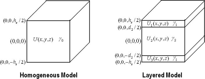
The homogeneous and the layered geometry.
In EIT, the forward problem is to find the voltage on the surface of the body given the current density distribution applied to the surface of the body with known admittivity distribution inside the body (Mueller et al. 1999). We formulate the forward problem as follows: If U(x, y, z) is the electric potential, J*(x, y, z) is the applied current density,(’*’ is either ‘T’ for top or ‘B’ for bottom), and γ(x, y, z) = γ is the internal admittivity distribution in the body Ω, then U(x, y, z) satisfies
| (1a) |
| (1b) |
| (1c) |
| (1d) |
| (1e) |
where ν is the outward normal at a point on the surface. The applied current is decomposed into its Fourier series:
| (2) |
Here, F is the number of terms used in the series expansion.
We solve the problem using the method of separation of variables. The three layered forward voltage obtained by decomposition using the eigenfunctions of the ave-gap model (Mueller et al. 1999), can be expressed as:
where i = 1,2 and 3 for different layers of the body. U1(x, y, z) is the electric potential in the top skin layer, U2(x, y, z) is the electric potential in the middle breast tissue layer and U3(x, y, z) is the electric potential in the bottom skin layer. Here,
| (3) |
The interfacial conditions for the layered case to be taken into account are that U(x, y, z) has to be continuous across layers and . We get six equations from these interfacial and boundary conditions, which we solve simultaneously assuming a step-wise constant admittivity in the layers to get the six coefficients A1, A2, A2, B1, B2 and B3 that define the forward voltages in the three layers.
| (4a) |
| (4b) |
| (4c) |
| (4d) |
| (4e) |
| (4f) |
Using the ave-gap model (Mueller et al. 1999), we obtain the voltages on the top and bottom electrode array denoted by VT and VB by integrating and respectively over the surface of each electrode and dividing by the area of the electrode.
Having solved the forward problem, our next step is to compare the results from the layered and the homogeneous forward solvers. The complete data set in EIT consists of linearly independent current patterns varying in spatial frequency applied to the body and the corresponding measured voltage patterns. We look at the relative drop in the impedance seen by the two models for increasing spatial frequency of the applied current patterns. We apply a set of optimal current patterns which maximize the distinguishability (Gisser et al. 1990). These optimal current patterns are the eigenvectors of the Neumaan to Dirichlet map for the geometry. The voltage patterns calculated from the forward solution would then just be a scaled version of the current patterns, the scale factors being the eigenvalues. These eigenvalues are in fact the impedances seen by the patterns. In our finite difference simulation of the layered model the lengths along the x-, y-, and z-axes were 5.5 cm, 6.6 cm and 4 cm, respectively. The thickness of each skin layer was 0.2 cm. The breast tissue (γ2) and skin (γ1) admittivities are 1 + 0i S/m and 0.1 + 0i S/m respectively. The homogeneous model simulation maintains the same dimensions as the layered simulation but has a constant admittivity of 1 + 0i S/m in all three layers. In Fig. 2 we see that the percent drop in impedance as we move to higher spatial frequency patterns from the lower ones is approximately 62.5% for the layered model while it is 89% for the homogeneous model. This shows that the layered model is less sensitive to the applied spatial frequency.
Figure 2.
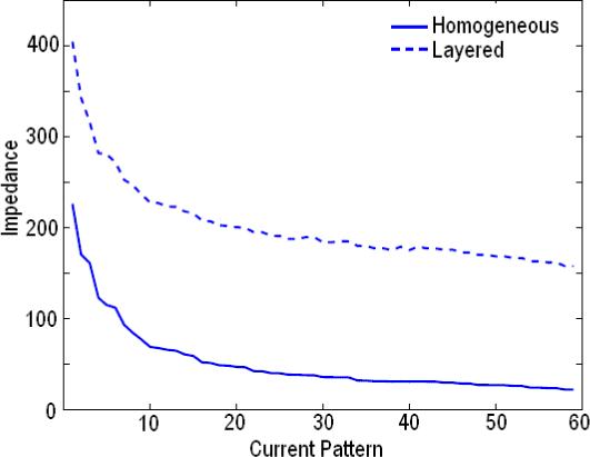
Eigenvalues for the Layered and Homogeneous Model.
3. Iterative estimation
In the homogeneous model, the forward voltage is calculated using a uniform admittivity of 1 and then scaled by the admittivity γ0, that gives the best fit between the computed forward voltages and the measured voltage data (Kao 2005). In the layered case, we follow an iterative optimization approach to estimate the two admittivities γ1 and γ2, that minimize the error between the computed forward voltages and the data measured from a layered medium. We define the error vector , which is a function of γ1 and γ2 as,
| (5) |
for i = 1, 2, ..K, where K is the number of linearly independent current patterns. We use the MATLAB optimization routine ’lsqnonlin’, which solves non-linear least squares problems, to minimize the L2-norm of error vector . This routine varies γ1 and γ2 and calculates the corresponding Uγ1,γ2 and Eγ1,γ2 to iteratively minimize norm of . The value of γ1 and γ2 thus obtained from this optimization procedure is used to calculate the layered forward voltages. This optimization assumes that the thicknesses of the layers is known, though multiple iterations of the optimization can be performed with different thickness values to find the values that produce the overall minimum error vector norm.
We have tested our iterative procedure for robustness and accuracy using experimental data. We validated our estimation procedure with experimental data acquired using ACT4. We built a layered phantom with agar forming the low admittivity skin layers and saline solution forming the high admittivity breast tissue. We modified the breast shaped phantom tank constructed previously (Kim et al. 2007) having two planar 30 electrode arrays on each side of the tank, by attaching two 0.5 cm thick agar layers to each side of the tank from the inside. These agar layers were formed by pouring the hot agar mix into molds that were constructed with the electrode array on one side. The solidified agar sheets were never removed from the electrode arrays, ensuring excellent contact and adhesion. In Fig. 3 we see the phantom with the two white agar sheets attached to the electrode arrays along with the space that is later filled with saline solution. In the figure we also see a conductive target which was introduced later to test the reconstruction algorithm. In order to minimize the agar admittivity, we filled the phantom tank with distilled water and left it overnight. This step results in ions diffusing out of the agar and reduces its admittivity. The conductivity of the distilled water measured the next day increased to 30 mS/m from an original value of 0 mS/m, indicating that the agar had become more resistive. The admittivity of the agar when the experiment was performed was in the range of 60 to 70 mS/m. The distilled water was removed and replaced by a saline solution with admittivity 210 mS/m. The estimation procedure returned values of 58 mS/m for γ1 and 176 mS/m for γ2. We calculate the forward voltages for the layered model using these estimated values. For the homogenous model the constant admittivity value γ0 was found to be 87 mS/m. We plot the dot product of the applied current pattern and the resulting voltage pattern for all applied current patterns, for the two models and the measured experimental data in Fig. 4. We see from the figure that the forward voltages calculated using these estimated values with the layered model fit the measured data better than the forward voltages from the homogeneous model.
Figure 3.
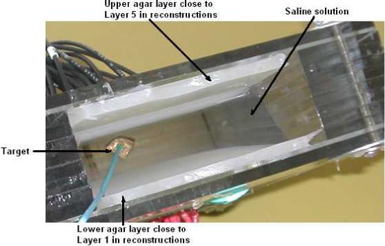
Agar + Saline layered phantom.
Figure 4.
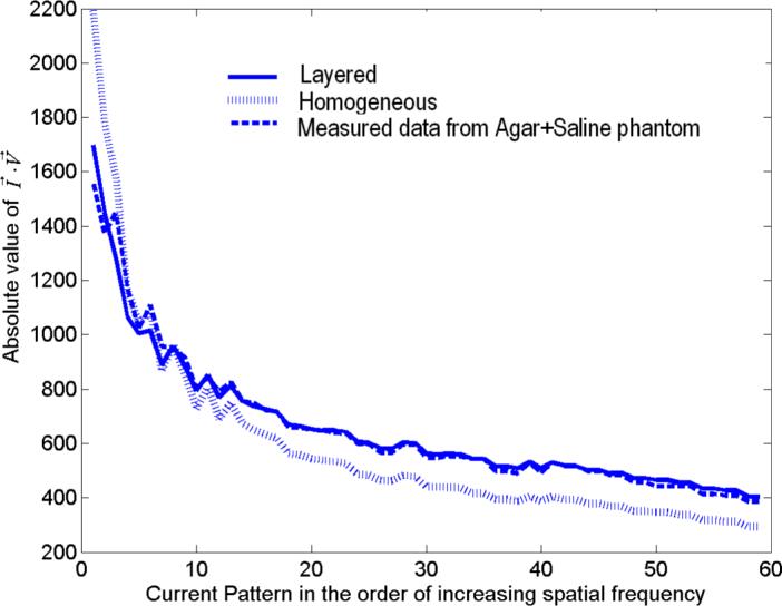
Comparison of the forward voltages calculated from the layered and homogeneous models with measured data from the agar+saline layered medium.
4. Clinical Studies
Having verified that our estimation procedure works acceptably well with simulated and experimental data, we applied it to patient data. Here, the actual structure of the breast is not known but we can assess the improvement in the agreement between the voltages predicted by the forward model and the measured data by using the layered model rather than the homogeneous model. We acquired the patient data using ACT4 with radiolucent electrode arrays. These arrays are attached to the compression plates of a mammography unit enabling EIT and mammography data to be taken simultaneously and in register (Kao et al. 2007). Working with patient data poses a problem as the exact breast dimensions are unknown. In order to best model the breast, for every patient, we calculate the eigenvectors for the corresponding breast dimensions and use them as the current patterns to be applied. We start the iterative procedure using γ0 from the homogeneous forward solver as the initial guess for both γ1 and γ2. The overall dimensions for the forward solver are set to match the breast thickness of the patient that is obtained from the mammography unit. Since the optimal value for the thickness of the skin layer is not known we run our iterative estimation procedure for varying thicknesses of skin and optimize the skin thickness estimate by minimizing the error between the measured data and the voltages calculated using the estimated admittivities of skin and breast tissue. Fig 5 shows the norm error between the voltages measured from the patient and calculated voltages for one patient for different applied excitation temporal frequencies as a function of skin thickness. We see that changing the skin thickness varies the norm error considerably more at lower temporal frequencies than at higer temporal frequencies. In addition, the norm error is generally larger for lower temporal frequencies. Both of these observations can be attributed to the fact that skin has lower admittivity at lower temporal frequencies. This lower admittivity makes the norm error sensitive to changes in skin thickness and makes it more difficult to find the accurate estimate for the breast tissue admittivity. Based on these results we take the optimum skin thickness for our model for this patient as 2 mm.
Figure 5.
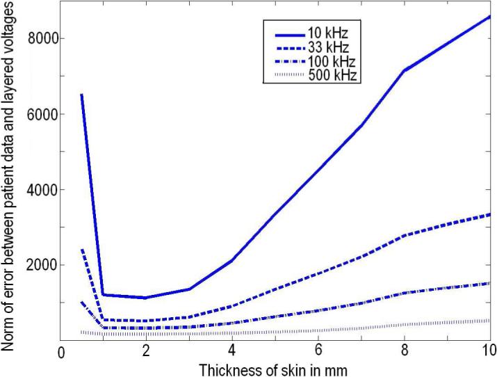
Skin thickness optimization for clinical data.
Fig. 6 provides a comparison of the skin and breast tissue admittivity estimated from the clinical data with those obtained from previously published work. The figure shows the real part of admittivity vs. the imaginary part of admittivity plotted for five frequencies 10kHz, 33kHz, 100kHz, 333kHz and 500kHz. In the figure, the dashed lines indicate patient data and solid lines indicate previously published data. The red dashed line represents estimated values of skin conductivity vs skin permittivity from patient data using our iterative estimation procedure which is compared with the red solid line which is plotted from data extracted from moist skin admittivity results published by Raicu (Raicu et al. 2000). The admittivity data was collected by Raicu, using an open-ended coaxial probe connected to a computer-controlled impedance analyzer. The breast largely consists of fatty adipose tissue which gives it its shape and size. The blue dashed line is a curve for the estimated values of breast tissue conductivity vs permittivity from patient data which is compared with the blue solid line which is derived from admittivity result for fatty adipose tissue from data published by Jossinet (Jossinet 1998). From the figure we see that the variation with frequency in the estimated skin admittivity from patients is much larger than the breast tissue admittivity and this result is validated by comparison to previously published data by Jossinet and Raicu.
Figure 6.
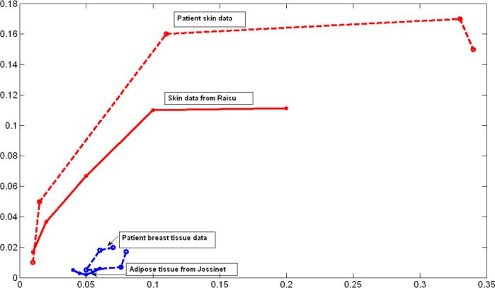
Comparative skin and breast tissue admittivity over a frequency range of 10 kHz to 500 kHz.
Finally we calculated the normalized norm of the difference between the layered and homogeneous model forward voltages and the patient data, and plotted it against frequency. Fig. 7 shows the percentage error between the clinical and forward model voltages that was calculated using the formula:
| (6) |
Fig. 7 thus shows the improvement that the layered forward model with the estimated admittivities provides over the homogeneous forward model for this clinical breast data.
Figure 7.
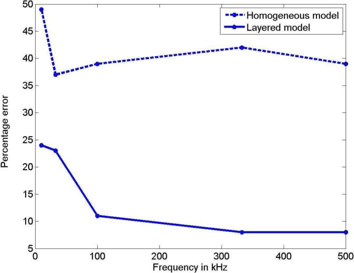
Improvement of the layered model over the homogeneous model vs. frequency for clinical data.
5. Reconstruction
We define the reconstruction problem in EIT as determining the electrical admittivity distribution γ(x, y, z), at all points (x, y, z) within the body, from measurements of the electric potential U(x, y, z) made on parts of the surface of the body upon application of an electric current density. The problem can also be defined in terms of applied voltages and measured currents. For a linearized reconstruction algorithm we assume that the admittivity distribution γ(x, y, z) differs only slightly from a constant value γ0 for the homogeneous model or the layer values (γ1 or γ2) for the layered model. This variation is represented by the perturbation η(x, y, z) (Mueller et al. 1999).With the ave-gap model, the linearized problem is to solve for η(x, y, z) in
| (7) |
for i, k = 1, 2, ...L − 1 linearly independent applied current patterns, where L is the number of electrodes. Uγ1,γ2 is the forward voltage calculated for a piecewise constant admittivity γ1 and γ2 in the skin and breast tissue layers, while V is the voltage measured at the electrodes. N is the number of voxels in the reconstruction. The volume associated with the nth voxel is denoted by Ωn. We define
| (8) |
as the A matrix and η as a vector of the perturbation admittivity values in the N voxels. We solve for η in this linearized system using:
| (9) |
The reconstruction problem is very ill-posed. We thereby use regularization (Kao 2005) to improve the reconstructions. The linear problem with regularization becomes:
| (10) |
where ε1 is a regularization parameter for NOSER type regularization and ε2 is for Tikhonov regularization.
We now study the reconstruction results for the layered model and compare them to those for the homogeneous model with simulated and experimental data. We will display the reconstruction of the breast tissue layer, excluding the thin skin layers, as breast tissue is the region of interest where most tumors are expected. The mesh we use for reconstructions is shown in Fig. 8. The thin layers in orange on the top and bottom are the skin layers which we do not show in the reconstruction. The five cross-sectional slices labeled slice 1 through slice 5 constitute the breast tissue layer. The numbering of the slices in the reconstruction goes from 1 for the bottom-most slice to 5 for the top-most slice. In the case of simulated data we use a finite difference forward model for a layered medium with a target embedded within it. The body geometry and the breast tissue and skin admittivities used were the same as those used earlier (1+0i and 0.1+0i S/m). The dimensions of the target were 1.1 × 1.2 × 1.0 cm3 and its admittivity was 100 S/m. Fig. 9 shows the location of the target in the body tissue region of the simulated layered structure. As shown, the target was placed in the top left corner of the breast tissue region which is divided into the five slices for the purpose of showing the target's location with respect to the reconstruction slices. The homogeneous reconstruction uses the homogeneous forward solution in the computation of the D and A matrices and the admittivity distribution in the reconstruction is perturbed from the constant value γ0. Fig. 10 shows a sketch of the location of the target relative to the reconstruction slices and the homogeneous model and layered model reconstructions. In the homogeneous reconstruction we see that the first and fifth slice have a lower admittivity as compared to the middle three slices, indicating the effect of skin on this region. The homogeneous reconstruction is centered around 1000 mS/m, with a range of 0 to 2000 mS/m. This large dynamic range can be attributed to the large skin to breast tissue admittivity ratio in case of this simulated data which is 1:10. The reconstruction in the layered case, uses the layered forward solution in the computation of the D and A matrices and perturbs the admittivity distribution from the estimated breast tissue admittivity value γ2. This reconstruction is centered around an admittivity of 1002 mS/m, differing only slightly from the actual breast tissue admittivity of 1000 mS/m. The layered reconstruction makes the target appear in the left corner in the 4th and 5th slices of the reconstruction, which maps on to the top left corner of the mesh.
Figure 8.
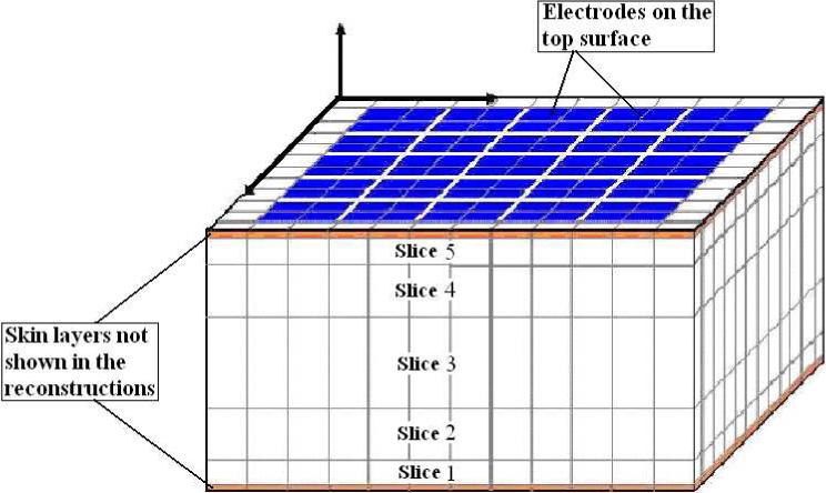
Voxel mesh used in the reconstruction.
Figure 9.
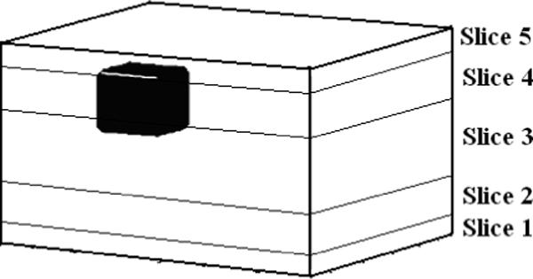
Finite Difference target geometry to be reconstructed.
Figure 10.
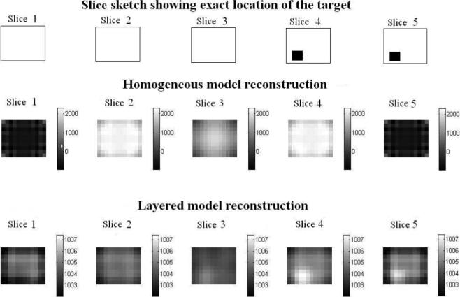
Layered and Homogeneous model reconstruction of simulated data for a target embedded in a layered structure in mS/m.
Next we check the performance of the layered model in detecting a target in the agar+saline layered medium described previously. Fig. 11 shows a sketch of the layered medium with the location of the target specified.
Figure 11.
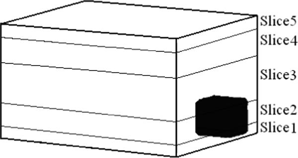
Diagrammatic representation of the agar+saline structure with target.
Fig. 12 shows a sketch of the location of the target relative to the reconstruction slices in the homogeneous model and layered model reconstructions. These reconstructions use the forward solutions calculated from the respective models in computation of the D and A matrices. The homogeneous reconstruction values vary from 80 mS/m to 82.5 mS/m with γ0 value of 81 mS/m. The layered reconstruction varies from 175 to 178.5 mS/m about the estimated breast tissue admittivity of 176 mS/m. We validate the target location in the right corner of slices 1 and 2 in the reconstruction by comparison with that in the sketch. The layered reconstruction appears better in contrast and shows the target better in slice 1 and slice 2. To further illustrate the improved contrast for the target with the layered model, we plot the conductivity difference along a cross-sectional line through the slice where the target is present and compare that to the conductivity difference in a cross-sectional line with no target, for the layered and the homogeneous reconstructions. We define the conductivity difference as: Conductivity difference (Δγ) = γvoxel − γmin where, γvoxel is the conductivity value of a voxel in the reconstruction and γmin is the value of minimum conductivity in the reconstruction. The solid lines in the figure show the difference with target, red for homogeneous model and blue for layered model. We chose the fourth row from the top in slice 2 which has the target present. The dashed lines show the condictivity difference without the target, again red being for homogeneous model and blue for layered model. We chose the fourth row from top from slice 4 where there is no target. We see from Fig. 13 that the difference for the homogeneous model with and without the target is small, both being around 0.3 to 0.4 mS/m. In the layered case however, the conductivity difference is about 1.9 mS/m in the place where the target is present, while the conductivity difference is just 0.4 mS/m when the target is absent. This quantitative difference is apparently enough to visibly locate the target in the reconstruction image.
Figure 12.
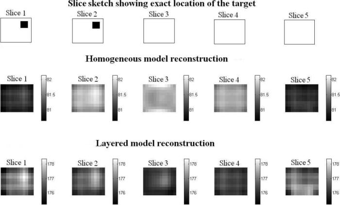
Layered and Homogeneous model reconstruction of a target embedded in agar+saline layered phantom in mS/m.
Figure 13.
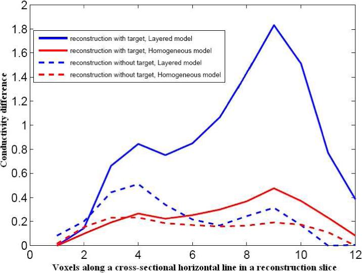
Conductivity difference comparison for layered and homogeneous model reconstructions with and without target.
6. Conclusion and Future Work
We have mathematically formulated and implemented a layered forward model which can account for thin low admittivity skin layers in breasts. We have incorporated this model into the inverse reconstruction problem and demonstrated the improvement that it produces in reconstructing targets embedded in layered bodies. We have developed an iterative algorithm to estimate the skin and breast tissue admittivities using the layered forward model and we plan to further explore analytical methods for the estimation of body and skin admittivities. So far we have worked with simulated and experimental data where the body geometry was always exactly known. We saw that dealing with clinical data poses many questions as each breast is different in terms of its size and thickness of the skin layers. We plan to carry out clinical studies to explore ways to better estimate the thickness and admittivities of the skin and breast tissue layers and thereby improve tumor detection.
7. Acknowledgments
This work was supported in part by CenSSIS, the Center for Subsurface Sensing and Imaging Systems, under the Engineering Research Centers Program of the National Science Foundation (award number EEC-9986821) and NIBIB, the National Institute of Biomedical Imaging and Bioengineering under (Grant Number R01-EB000456-03).
References
- Choi M, Kao T-J, Isaacson D, Saulnier G, Newell J. A simplified model of mammography geometry for breast cancer imaging with electrical impedance tomography. Engineering in Medicine and Biology Society. 2004;2:1310–1313. doi: 10.1109/IEMBS.2004.1403412. [DOI] [PubMed] [Google Scholar]
- Dobbins JT, Godfrey DJ. Digital X-ray tomosynthesis: current state of the art and clinical potential. Phys.Med.Biol. 2003;48(19):R65–106. doi: 10.1088/0031-9155/48/19/r01. [DOI] [PubMed] [Google Scholar]
- Gisser DG, Isaacson D, Newell J. Electric current compted tomography and eigenvalues. SIAM Journal on Applied Mathematics. 1990;50:1623–1634. [Google Scholar]
- Isaacson D, Cheney M, Newell J, Simske S, Goble J. NOSER: An algorithm for solving the inverse conductivity problem. Imaging Systems and Technology. 1990;2:66–75. doi: 10.1002/ima.1850020203. [DOI] [PMC free article] [PubMed] [Google Scholar]
- Isaacson D, Edic P. An algorithm on impedance imaging. IEEE EMBC. 1992;14:1693. [Google Scholar]
- Jossinet J. The impedivity of freshly excised human breast tissue. Physiol Meas. 1998;19:61–75. doi: 10.1088/0967-3334/19/1/006. [DOI] [PubMed] [Google Scholar]
- Kao T-J. PhD thesis. Troy, NY: 2005. A 3-D reconstruction algorithm for electrical impedance tomography using planar electrode arrays. [Google Scholar]
- Kao T-J, Saulnier GJ, Xia H, Tamma C, Newell JC, Isaacson D. A compensated radiolucent electrode array for combined EIT and mammography. Physio.Meas. 2007;28:291–299. doi: 10.1088/0967-3334/28/7/S22. [DOI] [PMC free article] [PubMed] [Google Scholar]
- Kim BS, Isaacson D, Xia H, Kao T, Newell JC, Saulnier GJ. A method for analyzing electrical impedance spectroscopy data from breast cancer patients. Physio.Meas. 2007;28:234–246. doi: 10.1088/0967-3334/28/7/S17. [DOI] [PMC free article] [PubMed] [Google Scholar]
- Mueller J, Isaacson D, Newell J. A reconstruction algorithm for electrical impedance tomography data collected on rectangular electrode arrays. IEEE trans. on Biomedical Imaging. 1999;46:1379–1386. doi: 10.1109/10.797998. [DOI] [PubMed] [Google Scholar]
- Raicu V, Kitagawa N, Irimajiri A. A quantitative approach to the dielectric properties of the skin. Phys.Med.Biol. 2000;45:L1–L4. doi: 10.1088/0031-9155/45/2/101. [DOI] [PubMed] [Google Scholar]
- Saulnier GJ, Ning L, Tamma C, Xia H, Kao T, Newell J, Isaacson D. An electrical impedance spectroscopy system for breast cancer detection. 29 th IEEE EMBS Annual International Conference; Lyon, France. 2007. [DOI] [PubMed] [Google Scholar]


