Homeomorphic Brain Image Segmentation with Topological and Statistical Atlases

Abstract

Atlas-based segmentation techniques are often employed to encode anatomical information for the delineation of multiple structures in magnetic resonance images of the brain. One of the primary challenges of these approaches is to efficiently model qualitative and quantitative anatomical knowledge without introducing a strong bias toward certain anatomical preferences when segmenting new images. This paper explores the use of topological information as a prior and proposes a segmentation framework based on both topological and statistical atlases of brain anatomy. Topology can be used to describe continuity of structures, as well as the relationships between structures, and is often a critical component in cortical surface reconstruction and deformation-based morphometry. Our method guarantees strict topological equivalence between the segmented image and the atlas, and relies only weakly on a statistical atlas of shape. Tissue classification and fast marching methods are used to provide a powerful and flexible framework to handle multiple image contrasts, high levels of noise, gain field inhomogeneities, and variable anatomies. The segmentation algorithm has been validated on simulated and real brain image data and made freely available to researchers. Our experiments demonstrate the accuracy and robustness of the method and the limited influence of the statistical atlas.

1. Introduction

The segmentation of medical images into separate structures and organs often requires the incorporation of prior information. Current methods, such as active shape and active appearance models, model the variability of spatial and intensity information into statistical atlases (Cootes et al., 1998; Leemput et al., 1999; Leventon et al., 2000; Rousson and Paragios, 2002; Tsai et al., 2004; Pohl et al., 2007; Heimann et al., 2007; Lu et al., 2007; Akselrod-Ballin et al., 2007). Relational information has also proven to be an important component, and has been incorporated into the modeling using covariance matrices (Fischl et al., 2002), fuzzy relations (Ciofolo and Barillot, 2005; Nempont et al., 2007), hierarchical models (Davatzikos et al., 2003; Rousson and Xu, 2006) or graph representations (Corso et al., 2007).

In a typical scenario, the atlas is transformed to match the image of interest, and a statistical classification method combines the atlas and image information to segment the structures (Leemput et al., 1999). An alternative is to perform a non-rigid registration of a single atlas or a deformable statistical atlas to the image and then transfer the segmentation labels (Christensen et al., 1997; Shen and Davatzikos, 2002; Rohde et al., 2003; Tsai et al., 2004). Hybrid methods incorporating statistical atlases, active shape models and/or non-rigid registration have also been proposed (Ciofolo and Barillot, 2005; Pohl et al., 2005; Heimann et al., 2007).

In all cases, the prior information can introduce a bias toward images most similar to the atlas images. A balance has to be found between the number and variety of prior segmentations needed to build the atlas, the complexity of the shape model or deformation, and the actual image information (Yeo et al., 2007). In addition, most of the global and regional topological properties of the structures are ignored in these representations. For example, segmented structures may become disjointed or connect freely with neighboring structures, irrespective of the underlying anatomy. Several methods have been proposed to preserve topology in the case of a single object (Malandain et al., 1993; Han et al., 2003) or multiple, separate objects (Mangin et al., 1995; Bazin and Pham, 2007c). However, none of these methods is able to preserve the topology of groups of objects. Even if the topology of two objects is invariant, the topology of the union of these objects is not constrained and can be arbitrary (see Fig. 1). In our previous work on the topology-preserving segmentation of brain tissue types (Bazin and Pham, 2007c), we managed to prevent these topology changes by constraining the objects to have nested interfaces, similarly to the original approach of (Mangin et al., 1995). Such constraints quickly become unrealistic when dealing with multiple structures rather than a few tissue types. On the other hand, the true anatomy typically follows strict topological relationships, which should inform the segmentation.

Fig. 1.

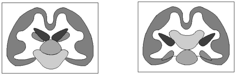
Importance of the topology of groups: the individual structures in above images have the same topology, but the relationships between them are different, corresponding to changes in the topology of groups (unions) of structures.

In this paper, we show that topological constraints on both the structures and their groups can be used to encode continuity and relationships without significantly biasing shape toward the anatomy of specific subjects. We present a strictly homeomorphic atlas-based segmentation algorithm and apply it to the segmentation of the major structures of the brain in magnetic resonance (MR) images. Our method employs only a coarse statistical atlas of the shape, deriving the segmentation predominantly from the image and topological constraints. Intensity distributions are iteratively estimated from the data, making the framework largely independent of the imaging modality as long as sufficient contrast exists to differentiate each structure. With this approach, we can segment the main cortical and subcortical structures of the brain all at once, accurately and reliably, without relying on complex prior models. In fact, our validation experiments indicate that the choice of images to be used in the atlas has little impact on the results.

This article presents the theoretical basis of our segmentation framework, describes our statistical and topological atlas of the human brain, and details the complete algorithm. Experimental validation include results on the robustness of our algorithm to noise and inhomogeneity, its sensitivity to atlas selection, as well as its accuracy on multiple image contrasts. A first overview of the method was presented in (Bazin and Pham, 2007a) along with a preliminary validation. This new article introduces several improvements of the method (see Sections 2.1, 2.3 and 4.3), provides additional algorithmic details (e.g. Sections 2.2, 4.1, 4.4) and validates the improved algorithm with an extensive set of experiments (see Section 5).

2. Methods

We seek to recover a set of K anatomical structures from a MR image, given a priori information about their shape and topology. Our segmentation methodology is based on three components: a fuzzy classification technique which attributes a membership value for all possible structures at every image point, a topology-preserving fast marching method which evolves the hard segmentation to fit the membership values, and a homeomorphism criterion which ensures that the topology of the segmentation is preserved during the evolution.

To segment an image, statistical and topological atlases are first registered to the image and membership values are estimated for each structure. The segmentation, initialized as the topology atlas, is then ’thinned’, leaving out regions with low membership for the segmented structure. A ’growing’ step expands all segmented structures on the regions of high memberships. Both steps preserve topology, yielding a segmentation that is consistent with the membership values. The algorithm then iteratively updates the atlas registration, membership estimation and topology-preserving evolution of the segmentation until convergence. We describe here the three main components of the method, while Sections 3 and 4 detail the atlas and the complete algorithm.

2.1. Tissue Classification

We extend the FANTASM (Fuzzy And Noise Tolerant Adaptive Segmentation Method) (Pham, 2001; Bazin et al., 2007a) approach to estimate membership values. Given the original image I, FANTASM minimizes the following energy function with respect to the fuzzy membership functions u_jk ∈ [0, 1], the gain field g_j, and the class centroids c_k:

$$E=\sum _{j,k}{u}_{j,k}^q\parallel g_j{I}_j-c_k\mid {\mid }^2+\frac{\beta }{2}\sum _{l\in N_j,m\ne k}{u}_{j,k}^q{u}_{l,m}^q,$$ (1)

for all structures k at all points j, with q > 1 a fuzziness factor (q = 2 in this work) and β a fixed smoothness parameter. The gain field is a smoothly varying function that we model as a low degree polynomial (see Bazin et al. (2007a) for details).

As with any tissue classification technique, difficulties arise if adjacent structures have the same or very close centroid values; the boundary between them becomes more sensitive to noise, and the boundaries with other structures may be incorrectly shifted. The additional information provided by a statistical atlas helps to remedy this issue but will also lower the influence of the signal intensity and blur the segmentation in areas of large variability between individuals. We make use of the relationship between structures to lower the influence of competing intensity clusters in regions that are spatially disconnected. We define the relationship set R_j to be the set of structures in contact at the boundary closest to the point j in the current hard segmentation (derived from the fuzzy memberships and the topology constraints, as detailed in Section 2.3). R_j is initialized on each structures boundary point as the set of structures in contact, and the sets are propagated inside the volume according to their relative distance to the boundary.

We incorporate the atlas and relationship information into FANTASM, resulting in the following energy function:

$$\begin{array}{l}{E}_S=\sum _{jk}\frac{u_{jk}^q}{r_{jk}}\parallel g_j{I}_j-c_k\mid {\mid }^2+\frac{\beta }{2}\sum _{l\in N_j,m\ne k}\frac{u_{jk}^q{u}_{lm}^q}{r_{jk}}\\ +\frac{\gamma }{2}\sum _{m\ne k}\frac{w_{km}{u}_{jk}^q{p}_{jm}^q}{r_{jk}}\end{array}$$ (2)

The first term in (2) is the data driven term, the second term enforces smoothness on the memberships, and the third term controls the influence of the statistical atlas (see Section 3). The parameters β and γ control the interplay of the different terms. The atlas is represented by a prior probability p_jk. The relationship function r_jk is defined to be

$$r_{jk}=\{\begin{array}{ll}1\hfill & k\in R_j,\hfill \\ p_{jk}\hfill & \text{otherwise}.\hfill \end{array}$$ (3)

The atlas weights w_km are defined as

$$w_{km}=\frac{s_w{({\sigma }_k+{\sigma }_m)}^2}{s_w{({\sigma }_k+{\sigma }_m)}^2+(1-s_w)\mid c_k-c_m{\mid }^2}$$ (4)

where ${\sigma }_k=\sqrt{\frac{{\sum }_j{u}_{jk}^q{(I_j-c_k)}^2}{{\sum }_j{u}_{jk}^q}}$ is an estimate of the standard deviation of intensity within k and s_w a scaling parameter. The weight w_km is close to one when c_k ≃ c_m but goes to zero when c_k ≠ c_m (w_km = s_w when |c_k − c_m| = σ_k + σ_m).

The relationship function penalizes against classes that are not connected to the class of the pixel j. For pixel classes corresponding to segmented structures distant from pixel j and with small prior probability p_jk, r_jk is set to that probability value, and the configuration is heavily penalized. The atlas weights allow the priors to influence the segmentation only where the intensity contrast between structures is low.

2.2. Digital Homeomorphisms

To ensure the topology is preserved, we need to guarantee that the segmented structures are related to the topological atlas by a homeomorphism. We recently introduced a digital homeomorphism criterion that extends the simple point criterion (Bertrand, 1994) to multiple objects and guarantees that the final segmentation and the topology atlas are homeomorphic in the continuous and digital domains (Bazin et al., 2007b). A ’simple point’ for a digital object is a point that can be exchanged with the object’s background without changing its topology. It can be detected locally by computing the number of connected components in its neighborhood: simple points must have only one connected object region and one connected background region in their neighborhood.

The improvement of digital homeomorphisms over the simple point criterion is essential for our task as it allows a more truthful representation of the anatomy. The criterion is given by the following:

The Digital Homeomorphism Constraint

A digital homeomorphism is a transformation that enforces, for a given segmentation of space into K objects O_k, that any sample point j may change from O_k to O_l if and only if j is a simple point for O_k, O_l, {O_k ∪ O_m}_{Om∩ Nj≠∅, m≠ k,l}, {O_l ∪ O_m}_{Om∩ Nj≠∅, m ≠ k,l}, {O_k ∪ O_m ∪ O_n}_{Om, On ∩ Nj≠∅, m,n ≠ k,l}, {O_l ∪ O_m ∪ O_n}_{Om, On ∩ Nj≠∅, m,n ≠ k,l} each considered as a single object (N_j is 26-neighborhood around j).

In other words, a point can change its segmentation label from k to l if it is a simple point for all groups of up to three objects including either O_k or O_l. The main difference with the single object case here is that simple points become object-dependent (see Fig. 2). The homeomorphism property holds regardless of the choice of connectivity.

Fig. 2.

Simple points for multiple objects: a) the central point can be exchanged between 2 and 4, but not 1 and 2 or 2 and 3 since these latter two cases would allow 1 and 3 to touch, b) the central point can swap from 1 to 3, but not 2 or 4, c) the central point is non-simple for any change if the objects are 6-connected, but can move from 3 to 2 if the objects are 26-connected (note that the groups 2–3 and 1–4 intersect each other in the latter case).

2.3. Topology-preserving Fast Marching Segmentation

The energy function of (2) is used to compute “soft” membership functions for each structure in a fashion similar to FANTASM (Pham, 2001). In addition, we compute a “hard” segmentation that is derived from the memberships but is constrained to be homeomorphic to the topology template.

The segmentation is performed using two successive iterations of a fast marching front propagation technique, first thinning the structures into a skeleton-like object and then growing the structures back to find the optimal boundary, using a minimal path strategy (Li et al., 2006; Bazin and Pham, 2007c). The speed function of the fast marching is a function of the memberships:

$$f_{jk}^{-}=\frac{u_{jk}}{{max}_m{u}_{jm}},f_{jk}^{+}=\frac{{max}_m{u}_{jm}}{u_{jk}}$$ (5)

where f⁻ is used in the thinning algorithm, and f⁺ in the growing algorithm. Note that this speed function integrates geometric smoothing in the propagation without additional curvature terms: when inside a structure, f⁻ = f⁺ = 1 and the fast marching behaves like a geometric distance function.

The goal of the thinning is to remove the regions, or equivalently to grow the boundaries, where the segmentation least reflects the underlying memberships. Starting from the current segmentation, we propagate the boundaries inside each structure by following the lowest values of f⁻. The thinning is stopped when the volume remaining inside each structure is below a given fraction v_th of the original volume (empirically set to 0.5, as a trade-off between robustness and convergence speed). The extended boundary region obtained defines the region to be updated in the growing algorithm.

Because of the strict homeomorphism requirements (described in detail in Section 2.2), the actual segmentation can only exchange labels. When the boundary for k is propagated inside the structure at j, it may change the segmentation label from k to m only if u_jm = max_lu_jl and the segmentations with label k and label m at j are homeomorphic. Note that no topological constraints are imposed on the thinned structures or the boundary region.

The growing algorithm starts from the boundaries of the thinned structures, and propagates them along the lowest values of f⁺, until the boundary region is filled. As with the thinning, the segmentation may be updated when the boundary for k reaches a point j with a different label m if the two corresponding segmentations are homeomorphic.

3. Anatomical Atlases

The above algorithm is general, and could be applied to any medical image segmentation problem where image intensity drives the segmentation, given the appropriate anatomical atlases. As we are interested in the major structures of the brain, we created an atlas for the following structures: cerebral gray matter (CRG), cerebral white matter (CRW), cerebellar gray matter (CBG), cerebellar white matter (CBW), brainstem (BS), ventricles (VEN), caudate (CAU), putamen (PUT), thalamus (THA) and sulcal cerebrospinal fluid (CSF).

3.1. Statistical Atlas

The first component of our anatomical atlas is a statistical spatial atlas, which will help distinguish structures with similar intensities. The atlas is built from a set of manual delineations of the structures of interest. For each image in the atlas, the delineation is rigidly aligned with the current atlas image, and a smooth approximation of the probabilities is accumulated. The smoothing replaces the step edge at the boundary of each structure in their binary delineation by a linear ramp over a band of size ε. The accumulated prior p_jk represents the probability of being inside each structure as a function of the distance to its boundary and its variability over the atlas images, similarly to sigmoid-based representations (Rousson and Xu, 2006; Pohl et al., 2006). By taking all these factors into account, we expect to reduce the bias toward the mean shape of the atlas and allow the statistical atlas to only influence areas most likely to be inside each structure. Fig. 3 shows the statistical priors computed from 18 subjects of the IBSR V2 dataset (Worth, 1996). We found experimentally that our method does not greatly depend on the number of subjects, but requires ε to be rather large (ε = 10mm seemed sufficient in all tested cases). The atlas is based on rigid alignment of the delineations because the algorithm is limited to rigid transformations in order to preserve the topology of the digital atlas, once registered (see Section 4.2). The joint use of a simple, rigid alignment and a large boundary smoothing also decreases the variations between atlases built from different subjects and populations (while increasing the variations within an atlas), as noted in our validation experiments.

Fig. 3.

The statistical atlas derived from the IBSR V2 delineations.

3.2. Topological Atlas

The second component of our atlas is a description of the topology, encoded as a hard segmentation of the brain. Anatomical structures can have a very complex geometry, yet they all tend to have a very simple topology, such as that of a sphere or torus. Groups of tissues and organs in contact provide additional topological properties. For instance, it is often assumed that the cerebral cortex has a spherical topology, but this requires a grouping of cerebral gray and white matter, sub-cortical structures and ventricles.

Creation of an appropriate topology atlas is non-trivial: manual segmentations have arbitrary topology, and inferring topological properties from anatomical atlases is not straightforward. We derived our topology atlas from the mean segmentation obtained from the statistical atlas above, with additional manual and automated topology correction (Bazin and Pham, 2007b) based on anatomy textbooks. The topological properties of the obtained atlas (see Fig. 4) are summarized in Table 1.

Fig. 4.

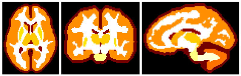
The topological atlas in axial, coronal and sagittal views.

Table 1.

Topological properties of the atlas

Structures	CSF	VEN	CBG	CRG	CAU	THA	PUT	BS	CBW	CRW
Components	1	1	1	1	2	1	2	1	2	1
Cavities	1	0	0	0	0	0	0	0	0	2
Handles	1	0	0	0	0	0	0	1	0	8

Even though most structures have spherical topology (no cavities or handles), there are a few exceptions. CSF entirely surrounds the brain, and shares a handle with the brainstem in the area of the fourth ventricle. Cerebral white matter is the most complicated, with two cavities holding the putamen, and a total of eight handles surrounding the ventricles and remaining sub-cortical structures. However, the group made of CRW and the sub-cortical structures (VEN, CAU, THA and PUT) has spherical topology as expected in the spherical brain hypothesis employed for cortical flattening (Thompson and Toga, 2002; Tosun et al., 2003). This model of topology effectively captures the relationships between structures as seen in structural MR images around 1mm resolution. Further analysis and testing of alternative models of brain topology may be needed as we incorporate additional structures or apply the method to different scales.

4. Algorithm

The complete algorithm is as follows:

1. Align atlases to image and set initial segmentation to the topological atlas.

2. Build the relationship sets R_j from the current segmentation.

3. Compute the memberships u_jk, centroids c_k and the inhomogeneity field g_j.

4. Thin structures using the fast marching algorithm with f⁻.

5. Grow back the structures using f⁺ and update the segmentation.

6. Refine the alignment of the atlases.

7. Loop to step 2 until convergence.

The convergence criterion is the relative amount of change in the energy E per iteration, which typically becomes lower than 10⁻³ in 10 to 20 iterations in the following experiments (approximatively 45 to 60 minutes). The overall complexity of the algorithm is O(N log N)+O(KN), with N the size of the image and K the number of structures.

4.1. Intensity and Tissue Initialization

The algorithm above is an iterative estimation technique, which requires an adequate initialization to converge. In particular, if the intensity centroids are poorly initialized, the method is likely to confuse neighboring structures. Approximate membership functions also need to be defined in order to register the atlases, depending on the image intensities alone.

To perform such initialization in a robust manner, we make use of predefined intensity profiles, which attribute a relative intensity value in [0, 1] for each structure in a given image MR contrast. Profiles have been empirically derived for T1-weighted, (SPGR and MPRAGE), T2-weighted and in PD, see Table 2. In these profiles, we also grouped structures of the same tissue type by giving them the same value (note that these groups can vary from image to image, with different contrasts).

Table 2.

MR contrast intensity profiles for tissue initialization

Structures	CSF	VEN	CBG	CRG	CAU	THA	PUT	BS	CBW	CRW
T1(SPGR)	0.2	0.2	0.5	0.5	0.5	0.7	0.7	0.9	0.9	0.9
T1(MPRAGE)	0.1	0.1	0.7	0.5	0.5	0.7	0.7	1.0	1.0	1.0
T2	0.9	0.9	0.6	0.6	0.6	0.6	0.6	0.5	0.5	0.5
PD	1.0	1.0	0.6	0.6	0.6	0.5	0.5	0.4	0.4	0.4

When segmenting an image of a given contrast, we first compute the robust minimum and maximum of the intensity (i.e. the intensity values at 1% and 99% of the histogram), normalize the image from these to [0, 1] and set the intensity clusters c_k to the prior profile values. We then perform a first estimation of the structures memberships, using only the intensity term in Eq.2 (β = γ= 0). When intensity clusters have the same value, the structures memberships are added, so that the memberships approximate a classification of the tissues rather than the structures.

4.2. Atlas Registration

During the segmentation, the statistical atlas must be registered to the image. We use a joint segmentation and registration technique (Pham and Bazin, 2006) that alternates between estimating the segmentation given the current atlas position, and then maximizes the following correlation energy with respect to T given the current segmentation:

$$E_R(T)=\sum _{jk}{p}_{T(j)k}^q{u}_{jk}^q.$$ (6)

where T is a rigid transformation.

The transformation is computed iteratively with a gradient ascent technique. The initial alignment is computed from the initial tissues memberships described above, and large pose variations are recovered with a Gaussian pyramid. After this initial alignment, a single scale is sufficient to refine the alignment during the segmentation.

Both the statistical and topological atlases are transformed into the image domain during the initial alignment, thus the possible transformations are restricted to preserve the topology on the digital grid. Note that continuous diffeomorphisms or general affine transforms do not preserve the digital topology (Bazin et al., 2007b). In practice, only rigid transformations can align the topological atlas correctly (given that the atlas has a minimum thickness of $\sqrt{3}$ voxels for all structures). After the initial alignment, one could increase the complexity of T, as it only affects the statistical atlas. However, our experiments using an affine transform for T did not yield any noticeable improvement in practice.

4.3. Multi-channel Images

In many studies, multiple image contrasts are acquired simultaneously, and may be combined to enhance the analysis. Although FANTASM is inherently multichannel, under the Euclidean norm each image channel is weighted equally, which may not be desirable. An improvement in multichannel performance can be obtained by a replacement of ||g_jI_j − c_k||² in Eq.2 with:

$$\sum _t\frac{{\sigma }_t^{-2}}{{\sum }_{\tau }{\sigma }_{\tau }^{-2}}\parallel g_{jt}{I}_{jt}-c_{tk}\mid {\mid }^2,$$ (7)

where ${\sigma }_t^2=\frac{{\sum }_{j,k}{u}_{jk}^2\parallel g_{jt}{I}_{jt}-c_{tk}\mid {\mid }^2}{{\sum }_{j,k}{u}_{jk}^2}$ is an estimate of the image variance for each contrast t.

4.4. Software

The algorithm described here has been integrated as a software plug-in in the Medical Image Processing, Analysis and Visualization (MIPAV) software package, a freely available and user-friendly image analysis program developed by the National Institutes of Health (McAuliffe et al., 2001) (http://mipav.cit.nih.gov/). The plug-in complements a set of neuroimage processing tools we recently released (Bazin et al., 2007a; Bazin and Pham, 2007b) and is freely available from: http://medic.rad.jhu.edu/download/public/. The software is a cross-platform Java application, and will be maintained and improved through regular releases and user feedback forums. Source code is not currently provided but may be released at a later time.

The software tool implements the entire segmentation pipeline, handles multiple channels and is distributed with the anatomical atlas described in Section 3. Default parameters were determined empirically, and can be easily tuned through a simple user interface (see Fig 5). The plug-in can be called from the graphical interface or from scripts for batch processing.

Fig. 5.

The segmentation software: original image, user interface (image and parameter panels) and result.

5. Experimental Validation

The experiments conducted in (Bazin and Pham, 2007a) mostly validated the algorithm accuracy on standard simulation phantoms and image databases. We present here, besides these results for the improved algorithm, additional experiments on multi-channel segmentation, and a more in-depth assessment of the impact of the statistical atlas on the segmentation. Unless otherwise stated, the default set of parameters was used for all experiments: spatial smoothing β = 0.1, atlas weight γ = 4.0, fuzziness coefficient q = 2, atlas-intensity scaling s_w = 0.1, thinning volume limit v_th = 0.5.

5.1. Simulated Images

A first set of experiments was conducted with the Brain-web phantom (Collins et al., 1998): several levels of noise and field inhomogeneity were simulated for T1 and T2-weighted modalities and the corresponding images segmented separately and using the multichannel option. The statistical atlas was derived from the 18 manually segmented images of the IBSR V2 data set. As the original Brainweb ground truth is only concerned with tissues (gray matter, white matter, cerebrospinal fluid), we performed a manual segmentation to separate cerebellum/brainstem, cerebrum and grouped sub-cortical structures. The results from the segmentation were grouped accordingly (CAU, PUT and THA as sub-cortical structures SUB, BS and CBW as CBS), and the difference measured with the Dice overlap measure ( $D(A,B)=\frac{2A\cap B}{A+B}$) and the average surface distance (in mm) between segmented structures, see Tables 3 and 4.

Table 3.

Dice overlap for the Brainweb dataset, for varying levels of noise and inhomogeneity.

Contrasts		Structures
		CSF	VEN	CBG	CRG	SUB	CBS	CRW
T1	Mean	0.916	0.895	0.879	0.916	0.812	0.721	0.940
	St. Dev.	0.009	0.003	0.007	0.015	0.018	0.008	0.013
T2+PD	Mean	0.909	0.856	0.856	0.818	0.691	0.676	0.781
	St. Dev.	0.016	0.019	0.010	0.065	0.014	0.018	0.101
T1+T2+PD	Mean	0.923	0.893	0.878	0.920	0.803	0.722	0.939
	St. Dev.	0.006	0.002	0.005	0.015	0.018	0.009	0.017

Table 4.

Average surface distance for the Brainweb dataset, for varying levels of noise and inhomogeneity (in mm).

Contrasts		Structures
		CSF	VEN	CBG	CRG	SUB	CBS	CRW
T1	Mean	0.353	0.623	1.933	0.389	1.267	1.514	0.377
	St. Dev.	0.030	0.006	0.031	0.042	0.053	0.048	0.053
T2+PD	Mean	0.319	0.984	2.272	0.757	2.116	2.533	2.111
	St. Dev.	0.055	0.163	0.099	0.234	0.049	0.049	1.298
T1+T2+PD	Mean	0.307	0.634	1.951	0.373	1.342	1.564	0.379
	St. Dev.	0.017	0.005	0.039	0.051	0.098	0.068	0.079

The Brainweb ’ground truth’ has arbitrary topology and our segmentation will always deviate from it because of the topological constraints it follows (the Euler characteristics for the Brainweb WM, GM and CSF tissue classes are 6, -1750 and -174 respectively). Despite this, the segmentation is very close to the Brainweb ground truth almost everywhere. The larger difference in CBS is due to the mean intensity of the brainstem, which is between the WM and GM intensities considered in Brainweb, and thus is not segmented as a homogeneous region in the ground truth. The topology enforces continuity for each structure, resulting in a segmentation very robust to high noise levels. The segmentation results for T2 and PD are less accurate, due to lower contrasts and PD and T2 images. Note however that the segmentation of CSF and CRG is enhanced by using the T2 and PD images with the T1, and the other structures remain very close to the results of T1 alone. The variation of accuracy with increasing levels of noise and inhomogeneity is small, due to the added robustness brought by the anatomical constraints.

5.2. Real Images

5.2.1. IBSR Evaluations

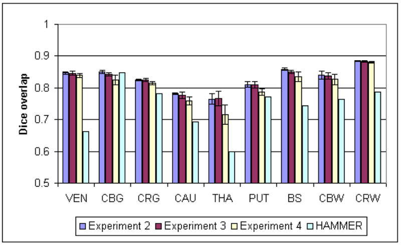
We tested the algorithm on the IBSR dataset, where we could compare each label individually (see Fig. 10). Because we used the same dataset to create the atlas, we designed four different experiments to measure the influence of a specific atlas on the method.

Fig. 10.

Example of segmentation from the IBSR dataset. From left to right, top to bottom: original image, computed segmentation, membership functions for CRW, CRG, CSF, VEN CAU, THA, PUT, BS, CBW, CBG, and 3D rendering.

In Experiment one, 8 images from the dataset were used to create the atlas, and the atlas parameter γ was varied from low to high while segmenting the remaining 10 images. In Experiment two, four atlases were generated with subsets of 18, 8, 3, and 1 images of the dataset, and used on the complete dataset. Note that in this experiment, the set of images used to build the atlas overlaps with the set of segmented images. In Experiment three, six separate subsets of 3 images were used to create atlases with no data in common, and run on the remaining images. Finally, Experiment four tested the potentially most biased option: a single image was used to generate the atlas, and the segmentation was run on all other images. As a comparison, we also performed a segmentation by non-rigid registration with HAMMER (Shen and Davatzikos, 2002), transferring the labels from the first IBSR image (note that the results of HAMMER should be compared to the case where a single image is used in building the atlas).

Dice overlap and average surface distance were measured for each segmented image and averaged over the segmented images. The results of Experiment one are displayed on Figs. 6 and 7. For Experiments two, three and four, we also compared the variation per subject (using the different atlases) and the variation per atlas (over the different atlases) in Tables 5 and 6).

Fig. 6.

Influence of the atlas coefficient over the overlap for the IBSR dataset.

Fig. 7.

Influence of the atlas coefficient over the average surface distance for the IBSR dataset.

Table 5.

Dice coefficients for the IBSR experiments

		Structures
		VEN	CBG	CRG	CAU	THA	PUT	BS	CBW	CRW
Atlas	Mean	0.850	0.852	0.824	0.781	0.773	0.817	0.862	0.849	0.887
01-18	St. dev	0.043	0.028	0.041	0.038	0.041	0.046	0.027	0.021	0.012
Atlas	Mean	0.846	0.843	0.827	0.786	0.750	0.814	0.854	0.823	0.884
01-03	St. dev	0.045	0.076	0.036	0.036	0.049	0.042	0.033	0.114	0.013
Atlas	Mean	0.842	0.853	0.829	0.782	0.783	0.797	0.859	0.840	0.882
01-01	St. dev	0.053	0.033	0.031	0.038	0.035	0.064	0.027	0.024	0.014
HAMMER	Mean	0.662	0.848	0.782	0.694	0.599	0.773	0.744	0.763	0.788
	St. dev	0.078	0.032	0.038	0.043	0.071	0.046	0.059	0.042	0.032
Exp.2	Mean	0.847	0.851	0.825	0.782	0.765	0.811	0.859	0.840	0.885
	St. dev Subject	0.047	0.041	0.037	0.037	0.042	0.050	0.027	0.045	0.013
	St. dev Atlas	0.005	0.015	0.006	0.007	0.019	0.016	0.014	0.020	0.004
Exp.3	Mean	0.845	0.842	0.824	0.778	0.767	0.809	0.850	0.838	0.884
	St. dev Subject	0.047	0.044	0.037	0.038	0.040	0.050	0.032	0.043	0.013
	St. dev Atlas	0.006	0.016	0.007	0.010	0.020	0.012	0.016	0.022	0.004
Exp.4	Mean	0.840	0.825	0.815	0.759	0.717	0.787	0.836	0.827	0.880
	St. dev Subject	0.049	0.039	0.037	0.049	0.046	0.056	0.034	0.048	0.014
	St. dev Atlas	0.011	0.027	0.009	0.023	0.034	0.024	0.025	0.031	0.005

Table 6.

Average surface distances in mm for the IBSR experiments

		Structures
		VEN	CBG	CRG	CAU	THA	PUT	BS	CBW	CRW
Atlas	Mean	0.778	1.222	0.900	0.939	1.486	0.968	1.102	0.895	0.682
01-18	St. dev	0.172	0.241	0.096	0.192	0.224	0.257	0.246	0.185	0.064
Atlas	Mean	0.821	1.298	0.909	0.901	1.619	0.979	1.155	1.068	0.703
01-03	St. dev	0.200	0.561	0.123	0.171	0.274	0.235	0.267	0.817	0.074
Atlas	Mean	0.838	1.248	0.905	0.956	1.423	1.049	1.135	0.930	0.715
01-01	St. dev	0.192	0.328	0.110	0.216	0.225	0.338	0.240	0.165	0.075
HAMMER	Mean	1.697	1.200	1.062	1.441	2.109	0.979	1.792	1.279	1.050
	St. dev	0.346	0.150	0.067	0.283	0.266	0.160	0.402	0.324	0.129
Exp.2	Mean	0.804	1.243	0.905	0.932	1.532	0.993	1.127	0.947	0.697
	St. dev Subject	0.187	0.336	0.107	0.188	0.245	0.272	0.238	0.336	0.069
	St. dev Atlas	0.050	0.110	0.018	0.043	0.119	0.074	0.109	0.130	0.025
Exp.3	Mean	0.810	1.300	0.909	0.951	1.530	1.005	1.197	0.967	0.702
	St. dev Subject	0.201	0.374	0.113	0.181	0.233	0.271	0.290	0.322	0.076
	St. dev Atlas	0.061	0.106	0.022	0.052	0.122	0.059	0.125	0.154	0.026
Exp.4	Mean	0.879	1.364	0.933	1.089	1.838	1.111	1.296	1.005	0.719
	St. dev Subject	0.229	0.302	0.109	0.300	0.260	0.295	0.302	0.318	0.085
	St. dev Atlas	0.112	0.161	0.026	0.139	0.207	0.127	0.196	0.210	0.033

The sulcal CSF is grouped with CRG and CBG in the IBSR segmentation, thus the overlap with the original ground truth are lowered for CRG and CBG and irrelevant for CSF. The algorithm recovers all structures with an accuracy significantly higher than the non-rigid registration approach and similar to the reported inter-rater scores of (Fischl et al., 2002). The overlap is somewhat lower for the sub-cortical structures (caudate, putamen and thalamus), due to their smaller size, variable intensities, and weak boundaries. Our segmentation results are also comparable and often superior to those reported by recent methods, see Akselrod-Ballin et al. (2007) for an extensive comparison.

Our experiments indicate that the choice of an atlas has a low impact on the segmentation. The atlas weight γ can vary over a large scale with little degradation of the results. For some structures (thalamus, brainstem, cerebral gray matter), the optimal weight seems to be even higher, but this is likely due to the fact that regions of varying intensities were combined when defining them in the atlas. In practice, we observed that a higher weight tends to increase the robustness on low resolution or noisy data, and that a lower weight tends to increase the adaptability on deformed or unusual anatomies. Using 18 rather than 3 or even 1 images to create the atlas did not yield a noticeable gain, and the fact that the images to segment were used in the atlas definition did not seem to influence the results. The results from the six different 3-images atlases appear equivalent for most structures, and even the atlases built from a single image had little effect on the segmentation (however, the results were slightly worse in that the variability was increased). These results demonstrate that the algorithm relies on the statistical atlas mostly to define the general regions where the structures should lie, and the actual boundaries are found based on the image intensities. The thalamus is the most sensitive structure to atlas variations, which can be explained by the fact that its boundary with surrounding white matter is very diffuse, and thus much more influenced by the atlas term than the image term. Using multiple delineations to build an atlas improves the segmentation, but not by a large amount. Only a few delineations are needed to capture most of the variability.

5.2.2. Comparisons and tests on other datasets

Finally, we tested the algorithm on various datasets from medical research studies, to demonstrate its robustness to different contrasts, resolutions, and anatomies (see Fig. 11). In a study on the effects of the drug methylenedioxymethamphetamine (MDMA), the Caudate and Putamen were independently delineated by experts on 9 images, and the algorithm achieved a Dice coefficient of 0.817 ± 0.024 for Caudate and 0.756±0.040 for Putamen. The average surface distances were 0.952 ± 0.209 for Caudate, 1.243 ± 0.219 for Putamen. The images were T1-weighted MPRAGE taken at 3T in which the Claustrum, a thin gray matter structure on the outer edge of the Putamen (see arrow in Fig. 11-a), was visible. For this reason, the Putamen was not as reliably extracted by the algorithm as in the validation experiments, as the atlas did not include the Claustrum in its model.

Fig. 11.

Examples of segmentation from research studies: a) subjects from a MDMA study, b) patients with Sturge-Weber Syndrome, c) subjects from the BLSA.

We also entered the algorithm in the caudate segmentation comparison (http://www.cause07.org/, van Ginneken et al. (2007)) consisting of several datasets to be segmented by different algorithms to be compared. The experiment was run with an increased smoothing β = 0.5 to compensate for the noise in some of the datasets. We appeared to get above average segmentation results on the pediatric dataset (average score of 84.98), and results very comparable to previously reported methods for the others. Interestingly, in one of the datasets (BWH-PNL), the caudate had been grouped with the nucleus accumbens in the delineations. Our usual atlas gave systematically worse results on the images of this set (average score of 46.75), but a modified atlas combining caudate and nucleus accumbens was successful in raising our score to the level of competing methods (average of 58.42). This outlines that even though the images used to create the atlas have a low impact on the segmentation, the delineation protocol will influence the results, so that similar but different protocols can be effectively encoded in the atlas.

To evaluate the performance of the algorithm on data with more extreme morphological abnormalities, the algorithm was visually evaluated on images of patients with Sturge-Weber Syndrome (SWS) and older subjects from Baltimore Longitudinal Study on Aging (BLSA). SWS is a neurological disorder that results in severe brain atrophy in children (Comi, 2003). Even for these dramatic cases clearly outside of a typical statistical atlas range, the algorithm provided a qualitatively adequate segmentation (Fig. 11-b). Subjects from the BLSA (Resnick et al., 2003) exhibited ventricle enlargement, cerebral atrophy, and loss of contrast between gray and white matter. As in the previous cases, the algorithm provided visually satisfying results (Fig. 11-c).

6. Discussion

In this paper, we introduced topological constraints as a robust and efficient prior for neuroimage segmentation. Topological properties of the tissues encode their continuity and relationships, independently of their shape. When combined with an efficient estimation scheme, they allow us to accurately segment cortical and sub-cortical structures of the brain without relying heavily on a statistical atlas. Our validation studies indicate that the choice of an atlas or the number of images involved in its creation have little influence on the segmentation. Thus, the influence of the atlas is minimized, and in our use, the method has not introduced any significant bias toward a specific subject or group of subjects, an essential requirement when considering the anatomical variability present in different neuroimaging studies. The method can be applied to various image contrasts, handles multi-modality segmentation, and is robust to large variations of the subject’s anatomy. Finally, the algorithm guarantees that the obtained segmentations are all homeomorphic to the topology atlas. This property is essential for further processing and analysis, for instance to produce conformal maps of the cortical surface or to analyze shape variations through diffeomorphisms.

The segmentation software is now in use in several research studies, and has been made freely available in the hope that other researchers will evaluate and adopt the tool. Recent brain segmentation methods have introduced many improvements in the definition of statistical atlases, and we are investigating the integration of the most promising approaches into our framework. We are also investigating the extension of the framework to handle pathologies that affect the topology of the brain such as tumors or lesions. Finally, we are studying the topological properties of more detailed parcellations of the brain to increase the number of structures we can automatically delineate.

Fig. 8.

Dice overlap coefficients for the IBSR experiments.

Fig. 9.

Average surface distances for the IBSR experiments.

References

- Akselrod-Ballin A, Galun M, Gomori J, Brandt A, Basri R. Prior knowledge driven multiscale segmentation of brain mri. Proceedings of the 9th International Conference on Medical Image Computing and Computer-Assisted Intervention (MICCAI’07); Brisbane. october, 2007. [DOI] [PubMed] [Google Scholar]
- Bazin PL, Cuzzocreo J, Yassa MA, Gandler W, McAuliffe M, Bassett S, Pham D. Volumetric neuroimage analysis extensions for the mipav software package. Journal of Neuroscience Methods. 2007a;165:111–121. doi: 10.1016/j.jneumeth.2007.05.024. [DOI] [PMC free article] [PubMed] [Google Scholar]
- Bazin P-L, Ellingsen L, Pham D. Digital homeomorphisms in deformable registration. Proceedings of the International Conference on Information Processing in Medical Imaging 2007 (IPMI’07); Kerkrade. july, 2007b. [DOI] [PubMed] [Google Scholar]
- Bazin P-L, Pham D. Statistical and topological atlas based brain image segmentation. Proceedings of the 9th International Conference on Medical Image Computing and Computer-Assisted Intervention (MICCAI’07); Brisbane. october, 2007a. [DOI] [PubMed] [Google Scholar]
- Bazin PL, Pham D. Topology correction of segmented medical images using a fast marching algorithm. Computer Methods and Programs in Biomedicine. 2007b;88(2):182–190. doi: 10.1016/j.cmpb.2007.08.006. [DOI] [PMC free article] [PubMed] [Google Scholar]
- Bazin P-L, Pham D. Topology-preserving tissue classification of magnetic resonance brain images. IEEE Transactions on Medical Imaging. 2007c;26(4) doi: 10.1109/TMI.2007.893283. special Issue on Computational Neuroanatomy. [DOI] [PubMed] [Google Scholar]
- Bertrand G. Simple points, topological numbers and geodesic neighborhood in cubic grids. Pattern Recognition Letters. 1994 october;15(10):1003–1011. [Google Scholar]
- Christensen GE, Joshi SC, Miller MI. Volumetric transformation of brain anatomy. IEEE Transactions on Medical Imaging. 1997 December;16(6):864–877. doi: 10.1109/42.650882. [DOI] [PubMed] [Google Scholar]
- Ciofolo C, Barillot C. Brain segmentation with competitive level sets and fuzzy control. Proceedings of the International Conference on Information Processing in Medical Imaging 2005 (IPMI’05); Glenwood Springs. july, 2005. [DOI] [PubMed] [Google Scholar]
- Collins DL, Zijdenbos AP, Kollokian V, Sled JG, Kabani N, Holmes C, Evans A. Design and construction of a realistic digital brain phantom. IEEE Transactions on Medical Imaging. 1998 june;17(3) doi: 10.1109/42.712135. [DOI] [PubMed] [Google Scholar]
- Comi A. Pathophysiology of sturge-weber syndrome. Journal of Child Neurology. 2003;18(8):509–516. doi: 10.1177/08830738030180080701. [DOI] [PubMed] [Google Scholar]
- Cootes TF, Edwards GJ, Taylor CJ. Active appearance models. Lecture Notes in Computer Science. 1998;1407:484–498. [Google Scholar]
- Corso JJ, Tu Z, Yuille A, Toga A. Segmentation of sub-cortical structures by the graph-shifts algorithm. Proceedings of the International Conference on Information Processing in Medical Imaging 2007 (IPMI’07); Kerkrade. july, 2007. [DOI] [PubMed] [Google Scholar]
- Davatzikos C, Tao X, Shen D. Hierarchical active shape models, using the wavelet transform. IEEE Trans Med Imaging. 2003;22(3):414–423. doi: 10.1109/TMI.2003.809688. [DOI] [PubMed] [Google Scholar]
- Fischl B, Salat DH, Busa E, Albert M, Dieterich M, Haselgrove C, van der Kouwe A, Killiany R, Kennedy D, Klaveness S, Montillo A, Makris N, Rosen B, Dale AM. Whole brain segmentation: Automated labeling of neuroanatomical structures in the human brain. Neuron. 2002;33:341–355. doi: 10.1016/s0896-6273(02)00569-x. [DOI] [PubMed] [Google Scholar]
- Han X, Xu C, Prince JL. A topology preserving level set method for geometric deformable models. IEEE Transactions on Pattern Analysis and Machine Intelligence. 2003 june;25(6):755–768. [Google Scholar]
- Heimann T, Munzing S, Meinzer H-P, Wolf I. A shape-guided deformable model with evolutionary algorithm initialization for 3d soft tissue segmentation. Proceedings of the International Conference on Information Processing in Medical Imaging 2007 (IPMI’07); Kerkrade. july, 2007. [DOI] [PubMed] [Google Scholar]
- Leemput KV, Maes F, Vandermeulen D, Suetens P. Automated model-based tissue classification of MR images of the brain. IEEE Transactions on Medical Imaging. 1999;18(10):897–908. doi: 10.1109/42.811270. [DOI] [PubMed] [Google Scholar]
- Leventon M, Faugeraus O, Grimson W. Proceedings of the Workshop on Mathematical Methods in Biomedical Image Analysis. 2000. Level set based segmentation with intensity and curvature priors; pp. 4–11. [Google Scholar]
- Li H, Yezzi A, Cohen L. 3D brain segmentation using dual-front active contours with optional user interaction. International Journal of Biomedical Imaging. 2006;2006:1–17. doi: 10.1155/IJBI/2006/53186. [DOI] [PMC free article] [PubMed] [Google Scholar]
- Lu C, Pizer S, Joshi S, Jeong J-Y. Statistical multi-object shape models. International Journal of Computer Vision 2007 [Google Scholar]
- Malandain G, Bertrand G, Ayache N. Topological segmentation of discrete surfaces. International Journal of Computer Vision. 1993;10(2):183–197. [Google Scholar]
- Mangin JF, Frouin V, Bloch I, Regis J, Lopez-Krahe J. From 3D magnetic resonance images to structural representations of the cortex topography using topology preserving deformations. Journal of Mathematical Imaging and Vision. 1995;5:297–318. [Google Scholar]
- McAuliffe M, Lalonde F, McGarry D, Gandler W, Csaky K, Trus B. Medical image processing, analysis and visualization in clinical research. Proceedings of the 14th IEEE Symposium on Computer-Based Medical Systems (CBMS 2001).2001. [Google Scholar]
- Nempont O, Atif J, Angelini E, Bloch I. Combining radiometric and spatial structural information in a new metric for minimal surface segmentation. Proceedings of the International Conference on Information Processing in Medical Imaging 2007 (IPMI’07); Kerkrade. july, 2007. [DOI] [PubMed] [Google Scholar]
- Pham D, Bazin P-L. Proceedings of the IEEE International Symposium on Biomedical Imaging. Arlington: april, 2006. Simultaneous registration and tissue classification using clustering algorithms. [Google Scholar]
- Pham DL. Spatial models for fuzzy clustering. Computer Vision and Image Understanding. 2001;84:285–297. [Google Scholar]
- Pohl KM, Fisher J, Bouix S, Shenton ME, McCarley RW, Grimson WEL, Kikins R, Wells WM. Using the logarithm of odds to define a vector space on probabilistic atlases. Medical Image Analysis. 2007;11:465–477. doi: 10.1016/j.media.2007.06.003. [DOI] [PMC free article] [PubMed] [Google Scholar]
- Pohl KM, Fisher J, Levitt JJ, Shenton ME, Kikins R, Grimson WEL, Wells WM. A unifying approach to registration, segmentation and intensity correction. Proceedings of the 8th International Conference on Medical Image Computing and Computer-Assisted Intervention (MICCAI’05); Palm Springs. october, 2005. [DOI] [PMC free article] [PubMed] [Google Scholar]
- Pohl KM, Fisher J, Shenton ME, McCarley RW, Grimson WEL, Kikins R, Wells WM. Logarithm odds maps for shape representation. Proceedings of the 9th International Conference on Medical Image Computing and Computer-Assisted Intervention (MICCAI’06); Copenhagen. october, 2006. [DOI] [PMC free article] [PubMed] [Google Scholar]
- Resnick SM, Pham DL, Kraut MA, Zonderman AB, Davatzikos C. Longitudinal MRI studies of older adults: A shrinking brain. Journal of Neuroscience. 2003;23(8):3295–3301. doi: 10.1523/JNEUROSCI.23-08-03295.2003. [DOI] [PMC free article] [PubMed] [Google Scholar]
- Rohde GK, Aldroubi A, Dawant BM. The adaptive bases algorithm for intensity-based nonrigid image registration. IEEE Transactions on Medical Imaging. 2003;22(11):1470–1479. doi: 10.1109/TMI.2003.819299. [DOI] [PubMed] [Google Scholar]
- Rousson M, Paragios N. Proceedings of the European Conference on Computer Vision, ECCV. 2002. Shape priors for level set representations; pp. 78–92. [Google Scholar]
- Rousson M, Xu C. A general framework for image segmentation using ordered spatial dependency. Proceedings of the 9th International Conference on Medical Image Computing and Computer-Assisted Intervention (MICCAI’06); Copenhagen. october, 2006. [DOI] [PubMed] [Google Scholar]
- Shen D, Davatzikos C. HAMMER: Hierarchical attribute matching mechanism for elastic registration. IEEE Transactions on Medical Imaging. 2002 november;21(11) doi: 10.1109/TMI.2002.803111. [DOI] [PubMed] [Google Scholar]
- Thompson P, Toga A. A framework for computational anatomy. Computing and Visualization in Science. 2002;5:1–12. [Google Scholar]
- Tosun D, Rettmann ME, Prince JL. Mapping techniques for aligning sulci across multiple brains. Proceedings of The Sixth Annual International Conference on Medical Image Computing and Computer-Assisted Interventions(MICCAI); Montral. Nov, 2003. [DOI] [PMC free article] [PubMed] [Google Scholar]
- Tsai A, III, WMW, Tempany C, Grimson WEL, Willsky AS. Mutual information in coupled multi-shape model for medical image segmentation. Medical Image Analysis. 2004;8:429–445. doi: 10.1016/j.media.2004.01.003. [DOI] [PubMed] [Google Scholar]
- van Ginneken B, Heimann T, Styner M. 3d segmentation in the clinic: A grand challenge. Proceedings of the 3D Segmentation in the Clinic: A Grand Challenge Workshop of the 9th International Conference on Medical Image Computing and Computer-Assisted Intervention (MICCAI’07); Brisbane. october, 2007. [Google Scholar]
- Worth A. Internet brain segmentation repository. 1996 http://www.cma.mgh.harvard.edu/ibsr/
- Yeo BT, Sabuncu MR, Desikan R, Fischl B, Golland P. Effects of registration regularization and atlas sharpness on segmentation accuracy. Proceedings of the 9th International Conference on Medical Image Computing and Computer-Assisted Intervention (MICCAI’07); Brisbane. october, 2007. [DOI] [PMC free article] [PubMed] [Google Scholar]