Covariate adjustment for two-sample treatment comparisons in randomized clinical trials: A principled yet flexible approach

SUMMARY

There is considerable debate regarding whether and how covariate adjusted analyses should be used in the comparison of treatments in randomized clinical trials. Substantial baseline covariate information is routinely collected in such trials, and one goal of adjustment is to exploit covariates associated with outcome to increase precision of estimation of the treatment effect. However, concerns are routinely raised over the potential for bias when the covariates used are selected post hoc; and the potential for adjustment based on a model of the relationship between outcome, covariates, and treatment to invite a “fishing expedition” for that leading to the most dramatic effect estimate. By appealing to the theory of semiparametrics, we are led naturally to a characterization of all treatment effect estimators and to principled, practically-feasible methods for covariate adjustment that yield the desired gains in efficiency and that allow covariate relationships to be identified and exploited while circumventing the usual concerns. The methods and strategies for their implementation in practice are presented. Simulation studies and an application to data from an HIV clinical trial demonstrate the performance of the techniques relative to existing methods.

1. INTRODUCTION

The primary objective of many randomized clinical trials is to evaluate the difference in mean outcome between two treatments. In typical moderate-to-large-scale trials, the setting addressed herein, in addition to the primary outcome, extensive baseline data are collected on each participant prior to treatment administration, such as baseline observations on the outcome and qualitative and quantitative variables reflecting demographics, prior medical and treatment history, and physiological status. Some of these baseline covariates may be related to the primary outcome and may exhibit chance imbalances between the two treatment groups.

A vast literature exists on whether or not and how to “adjust” the analysis of treatment difference for the effects of covariates in order to increase the precision of the estimator for this treatment effect, thereby increasing statistical power, and to take imbalances into account [1, 2, 3, 4, 5, 6]. Indeed, that many studies fail to meet their accrual goals and the desire to use the data from patient volunteers most efficiently are strong rationales for this practice. However, covariate adjustment has inspired considerable controversy among numerous authors [1, 7, 8, 9] and regulatory authorities [10, 11] because of the potential for biased estimation due to post hoc selection of covariates and, more ominously, the temptation for analysts to engage in a “fishing expedition” to find “the covariate model that best accentuates the estimate and/or statistical significance of the treatment difference” [1]. Thus, trialists and regulatory agencies have been reluctant to endorse adjusted analyses, and current guidelines assert strongly that, if adjustment is undertaken, only a few such covariates should be used, chosen based on prior knowledge of their prognostic value; and these should be prespecified in the protocol or analysis plan, as should be the form of the model relating covariates to outcome to be used for adjustment (e.g., [11, 12]). However, associations between covariates and outcome may not be appreciated at the design stage [1], particularly if such information was not collected systematically in previous studies, but may be evident only at the analysis stage, subsequent to unblinding. An unfortunate consequence of these recommendations may be that a critical opportunity to enhance efficiency and reveal important, real effects may be lost.

Clearly, approaches that seek to resolve the tension between the need to make the best use of the data and concerns over the properties of adjusted estimators and possible lack of objectivity are needed. Pocock et al. [1] strongly encourage research along these lines, arguing that covariate adjustment should be carried out whenever appropriate while simultaneously making “one’s statistical policy for covariate adjustment completely objective.” Some approaches in this spirit, such as that of Koch et al. [2], which does not require regression modeling of covariate effects, have been proposed. Nonetheless, to our knowledge, a general, practically-feasible strategy that achieves this goal has not been elucidated.

In this article, we consider covariate adjustment in estimation of treatment differences in randomized clinical trials from the formal point of view of semiparametric theory (e.g., [13]). This leads to characterization of all treatment effect estimators, facilitating comparisons among competing methods. Moreover, emerging elegantly from this perspective is principled adjustment methodology that supports objective incorporation of covariate effects while simultaneously exploiting covariate-outcome relationships to increase precision. Because the approach automatically separates modeling of these relationships from evaluation of the treatment effect, it obviates concerns over suspicious “data dredging” exercises.

In Section 2, we introduce a formal model framework and identify the parameter representing the treatment effect of interest. We present the semiparametric theory results in Section 3. In Section 4, based on the theory, we propose a practical strategy for adjusted analysis. The methods are applied to data from an HIV clinical trial in Section 5, and simulation studies demonstrating performance are summarized in Section 6.

2. FRAMEWORK AND SCOPE OF INFERENCE

Consider a clinical trial with n subjects sampled from a population of interest. Let Y denote the outcome on which the primary analysis will be based (continuous or discrete), and let Z = 1 or 0 with probabilities δ or 1 − δ indicating randomization to, e.g., experimental treatment or control. Let X (p×1) be a vector of baseline covariates; X may include a baseline measurement on Y and additional quantitative and qualitative characteristics recorded prior to treatment initiation. Randomization guarantees statistical independence of Z and X, written as Z ⫫ X, which is critical to our further developments. The observed data from the trial are (Y_i, Z_i, X_i), i = 1, …, n, independent and identically distributed (iid) across i.

Within this framework, we may identify unambiguously the “treatment effect” that is ordinarily targeted by the primary analysis, given by

$$\beta =E(Y|Z=1)-E(Y|Z=0),$$ (1)

i.e., the difference in mean outcome between the two treatments. This may be representedequivalently by E(Y|Z) = μ₀ + βZ, where μ₀ = E(Y | Z = 0); note that this is a model only for the mean outcome for each treatment, with no additional assumptions, such as normality or equal variances in the two groups, implied.

The usual treatment effect β in (1) is defined unconditionally; i.e., as the effect of treatment relative to control averaged across the population. An alternative measure of treatment effect is defined conditional on a subset of the population having the particular covariate values X,

$${\beta }_x=E(Y|Z=1,X=x)-E(Y|Z=0,X=x).$$ (2)

For continuous Y, a standard approach to estimate β_x is to postulate a linear regression model

$$E(Y|Z,X)={\gamma }_0+{\gamma }_X^{T}X+{\beta }_{Z}Z,$$ (3)

often referred to as the “analysis of covariance” (ANCOVA) model. Model (3) is a popular basisfor “covariate-adjustment,” where β_Z is interpreted as the “treatment effect after adjusting for the covariates X.” In (3), no interactions(s) are specified between elements of X and Z, so that (3) assumes that this “adjusted” treatment effect is constant across values of X. Models may also include such interactions; see Section 3. For other outcomes, alternative models and effect measures may be specified; for example, for binary Y, one may consider the logistic regression model

$$E(Y|Z,X)=\frac{exp({\gamma }_0+{\gamma }_X^{T}X+{\gamma }_{Z}Z)}{1+exp({\gamma }_0+{\gamma }_X^{T}X+{\gamma }_{Z}Z)},$$ (4)

where γ_Z denotes the log-odds ratio conditional on X, assuming that this conditional log-odds ratio is constant for all values x.

The unconditional treatment effect (1) is overwhelmingly the focus of the primary analysis in most randomized trials, with inference on conditional treatment effects as in (2) often specified as secondary analyses. However, this is a matter of some debate; some researchers advocate that the conditional treatment effect (2) is a more appropriate basis for primary inferences; e.g., Hauck et al. [12] “recommend that the primary analysis adjust for important prognostic covariates in order to come as close as possible to the clinically most relevant subject-specific measure of treatment effect.” Clearly, both unconditional and conditional treatment effects are of considerable and complementary importance in developing a comprehensive understanding of how treatments compare. The former provides a measure of overall effect useful for broad policy recommendations, which explains its role as the primary focus of regulatory authorities. Inference on the latter can reveal interactions between treatment and patient characteristics; qualitative such interactions (i.e, the direction of the effect changes depending on x) may have critical implications for use of the treatment in certain subpopulations.

With continuous outcome, this debate rarely receives explicit mention because, if (3) is an exactly correct representation of the relationship E(Y |Z, X), then β and β_x coincide. In fact, it is well-appreciated that, with Z ⫫ X, the least squares estimator for β_Z in (3) is consistent for β in (1) regardless of whether or not (3) is the correct representation and is generally more precise than competing estimators, e.g., the difference in sample means, which do not take covariates into account. In Section 3, we show that these results follow immediately from semiparametric theory. For binary and other outcomes where nonlinear regression models are natural, the distinction between the unconditional and conditional perspectives is pronounced [12]. E.g., γ_Z in (4) is generally different from the unconditional log-odds ratio in a logistic regression model not including X. Accordingly, in general, it is critical to state unambiguously the inference (unconditional or conditional) desired.

In this article, we do not enter into this debate. Rather, given the long-standing status of the unconditional treatment effect as the primary parameter of interest in most clinical trials, we focus henceforth on covariate adjustment in the context of inference on β in (1), with the goal of making this inference as precise as possible under very general conditions.

3. SEMIPARAMETRIC INFERENCE

We consider estimation of β based on the iid data (Y_i, Z_i, X_i), i = 1, …, n, under as unrestrictive conditions as possible. We make no assumptions on aspects of the joint distribution of (Y, Z, X), such as parametric assumptions on the distributions of Y given Z or Y given (Z, X) (e.g., normality and/or common variance) except that Z ⫫ X by randomization. We now show that semiparametric theory leads under these conditions to the class of all consistent and asymptotically normal estimators (“large n”) for β, including the “most precise.” As noted at the outset, we focus on moderate-to-large-sized trials, and we demonstrate in Section 6 that the implications of the asymptotic theory are relevant in this setting.

Under these conditions, when one of the elements of X is a baseline observation on Y, Leon et al. [14] and Davidian et al. [15] derive the class of all consistent estimators for β by appealing directly to semiparametric theory [13] or by making an analogy to missing data problems and using the semiparametric missing-data theory of Robins et al. [16]. We comment on this “missing data” analogy below. Because a baseline outcome is just another baseline covariate, these results are immediately applicable here and lead to the following.

Let the numbers of subjects randomized to experimental treatment and control be $n_1={\sum }_{i=1}^n{Z}_i$ and $n_0={\sum }_{i=1}^n(1-Z_i)$, n = n₀ + n₁. Write the sample means of outcome in each group as ${\overline{Y}}^{(1)}=n_1^{-1}{\sum }_{i=1}^n{Z}_i{Y}_i$ and ${\overline{Y}}^{(0)}=n_0^{-1}{\sum }_{i=1}^n(1-Z_i)Y_i$, with $\overline{Z}=n^{-1}{\sum }_{i=1}^n{Z}_i=n_1/n$ the sample proportion randomized to treatment. Then it follows from References [14, 15] that all reasonable consistent and asymptotically normal estimators for β either can be written exactly as or are asymptotically equivalent to an expression of the form

$${\overline{Y}}^{(1)}-{\overline{Y}}^{(0)}-\sum _{i=1}^n(Z_i-\overline{Z})\left\{n_0^{-1}{h}^{(0)}(X_i)+n_1^{-1}{h}^{(1)}(X_i)\right\},$$ (5)

where h^(k)(X), k = 0, 1, are arbitrary scalar functions of X.

When h⁽⁰⁾(X_i) = h⁽¹⁾(X_i) ≡ 0, (5) reduces to the sample mean difference Ȳ⁽¹⁾ −Ȳ⁽⁰⁾, the standard “unadjusted” estimator, which is unbiased and trivially consistent for β and asymptotically normal under our general conditions. From (5), all consistent and asymptotically normal estimators for β may be viewed as “augmenting” [17] this estimator by the second term, which incorporates covariates and thereby implements the “adjustment,” in a spirit similar to estimators proposed in the survey sampling literature [18, 19, 20]. Because Z ⫫ X by randomization, the “augmentation” term converges in probability to zero, so that (5) is consistent for β for any h^(k), k = 0, 1 (see the Appendix). The h^(k) thus reflect the nature of the adjustment, and distinctions among estimators and insight into their relative precision may be deduced from these functions, as we now describe.

As noted above, a popular adjusted estimator for β is the least squares estimator for β_Z in the ANCOVA model (3), which we denote as β̂_{ANCOV A1}, and it is widely accepted that β̂_{ANCOV A1} is consistent for β. It is straightforward to demonstrate (see the Appendix) that this estimator is asymptotically equivalent to an expression of the form (5) with

$$h^{(0)}(X_i)=h^{(1)}(X_i)={\mathrm{\sum }}_{XY}^T{\mathrm{\sum }}_{XX}^{-1}{X}_i,$$ (6)

$${\mathrm{\sum }}_{XY}=E[\{X-E(X)\}\{Y-E(Y)\}],{\mathrm{\sum }}_{XX}=E[\{X-E(X)\}{\{X-E(X)\}}^T],$$ (7)

the covariance between X and Y and the covariance matrix of X in the overall population, respectively. Because β̂_{ANCOV A1} is asymptotically equivalent to an estimator of form (5), we may conclude immediately that it is consistent for β and asymptotically normal under entirely unrestrictive conditions; normality of the outcome conditional on (Z, X), continuous outcome, or constancy of var(Y |Z, X) are not required. Indeed, the model (3) from which it is derived need not even be a correct representation of E(Y |Z, X) for these results to hold.

One could in fact use formulation (5) to estimate β directly by replacing Σ_XY and Σ_XX in (7) by estimators in (6); e.g., by the corresponding sample covariance matrices. Semiparametric theory [13, 14, 15] ensures that the asymptotic normal distribution of the resulting estimator will have variance identical to that achieved if Σ_XX and Σ_XY were known, reflecting a general result for estimators of form (5): substitution of consistent estimators for quantities appearing in the functions h^(k) does not alter the large sample properties, a feature we discuss further below. Thus, this strategy would yield an estimator asymptotically equivalent to β̂_{ANCOV A1}.

From (6), the h^(k)(X_i), k = 0, 1, associated with β̂_{ANCOV A1} are the same for each treatment and are linear functions of X_i, which, defining

$${\mathrm{\sum }}_{XY}^{(k)}=E[\{X-E(X)\}\{Y-E(Y)\}|Z=k],k=0,1,$$ (8)

and noting that ${\mathrm{\sum }}_{XY}=(1-\delta ){\mathrm{\sum }}_{XY}^{(0)}+\delta {\mathrm{\sum }}_{XY}^{(1)}$, may be written equivalently as

$$h^{(0)}(X_i)=h^{(1)}(X_i)={\{(1-\delta ){\mathrm{\sum }}_{XY}^{(0)}+\delta {\mathrm{\sum }}_{XY}^{(1)}\}}^T{\mathrm{\sum }}_{XY}^{-1}{X}_i.$$ (9)

Other familiar estimators may be shown to be asymptotically equivalent to estimators of form (5), with corresponding h⁽⁰⁾ = h⁽¹⁾ that, while still linear in X_i, is possibly different from (6) and (9). Consider an ANCOVA model like (3) but also including an interaction term between Z and X, which may be written in terms of centered versions of Y, Z, and X as

$$E\{Y-E(Y)|Z,X\}={\gamma }_X^T\{X-E(X)\}+{\gamma }_{XZ}^T\{X-E(X)\}\{Z-E(Z)\}+{\beta }_Z\{Z-E(Z)\},$$ (10)

and fitted by least squares regression of Y_i − Ȳ on X_i − X̄, Z_i − Z̄, and (X_i − X̄)(Z_i − Z̄), where $\overline{Y}=n^{-1}{\sum }_{i=1}^n{Y}_i$ and $\overline{X}=n^{-1}{\sum }_{i=1}^n{X}_i$ [21]. Model (10) may seem an inappropriate framework for estimating the unconditional treatment effect β, as the interaction term implies that the conditional treatment effect depends on the covariate and hence cannot equal the unconditional effect. However, Yang and Tsiatis [21] show for scalar X that the least squaresestimator for β_Z under (10) is a consistent and asymptotically normal estimator for β in (1); see also Reference [22]. This generalizes to vector X; we show in the Appendix that this estimator, denoted β̂_{ANCOV A2}, is asymptotically equivalent to an expression of the form (5) with

$$h^{(0)}(X_i)=h^{(1)}(X_i)={\{\delta {\mathrm{\sum }}_{XY}^{(0)}+(1-\delta ){\mathrm{\sum }}_{XY}^{(1)}\}}^T{\mathrm{\sum }}_{XY}^{-1}{X}_i.$$ (11)

Thus, that β̂_{ANCOV A2} is consistent for β and asymptotically normal under very general conditions is immediate and holds even if (10) is an incorrect representation of E(Y |Z, X).

Expressions (9) and (11) are identical if either δ = 0.5 or ${\mathrm{\sum }}_{XY}^{(0)}={\mathrm{\sum }}_{XY}^{(1)}$. Accordingly, under these conditions, β̂_{ANCOV A1} and β̂_{ANCOV A2} are asymptotically equivalent and hence equally precise (asymptotically). Otherwise, β̂_{ANCOV A2} has smaller asymptotic variance than β̂_{ANCOV A1}; in fact, this variance is the smallest among all estimators for which h(k)(X_i), k = 0, 1, are linear in X_i [14, 21, 22] (see the Appendix). Thus, any other linear h(k), k = 0, 1, including those where h⁽⁰⁾ ≠ h⁽¹⁾, correspond to estimators that can be no more precise than those involving the common h^(k) given in (11).

Koch et al. [2] propose an estimator for β given by

$${\widehat{\beta }}_{\mathit{KOCH}}={\overline{Y}}^{(1)}-{\overline{Y}}^{(0)}-V_{XY}^T{V}_{XX}^{-1}({\overline{X}}^{(1)}-{\overline{X}}^{(0)}),$$ (12)

where ${\overline{X}}^{(0)}=n_0^{-1}{\sum }_{i=1}^n(1-Z_i)X_i;{\overline{X}}^{(1)}=n_1^{-1}{\sum }_{i=1}^n{Z}_i{X}_i,$

$$V_{XY}=n_0^{-1}{\widehat{\mathrm{\sum }}}_{XY}^{(0)}+n_1^{-1}{\widehat{\mathrm{\sum }}}_{XY}^{(1)},V_{XX}=n_0^{-1}{\widehat{\mathrm{\sum }}}_{XX}^{(0)}+n_1^{-1}{\widehat{\mathrm{\sum }}}_{XX}^{(1)},$$ (13)

$$\begin{array}{c}{\widehat{\mathrm{\sum }}}_{XY}^{(k)}={(n_k-1)}^{-1}\sum _{i=1}^{n}I(Z_i=k)(Y_i-{\overline{Y}}^{(k)})(X_i-{\overline{X}}^{(k)}),\\ {\widehat{\mathrm{\sum }}}_{XX}^{(k)}={(n_k-1)}^{-1}\sum _{i=1}^{n}I(Z_i=k)(X_i-{\overline{X}}^{(k)}){(X_i-{\overline{X}}^{(k)})}^T,k=0,1,\end{array}$$ (14)

and I(·) is the indicator function. Noting that

$${\overline{X}}^{(1)}-{\overline{X}}^{(0)}=\frac{n}{n_0{n}_1}\sum _{i=1}^n(Z_i-\overline{Z})X_i,\frac{n}{n_0{n}_1}=n_0^{-1}+n_1^{-1},$$ (15)

it is easy to appreciate that β̂_KOCH is asymptotically equivalent to an expression of form (5), where $V_{XY}^T{V}_{XX}^{-1}$ is replaced by its limit in probability, so that β̂_KOCH is immediately seen to be consistent and asymptotically normal under our unrestrictive conditions. It is shown in the Appendix that this in fact leads to the h^(k), k = 0, 1, in (11). Thus, via semiparametric theory, we are led directly to the result that β̂_KOCH and β̂_{ANCOV A2} are asymptotically equivalent; moreover, as observed by Lesaffre and Senn [4], when n₀ = n₁ (approximately δ = 0.5), β̂_KOCH is approximately equivalent to the usual ANCOVA estimator β̂_{ANCOV A1}. Otherwise, in a large sample sense, Koch’s estimator is more precise.

Yang and Tsiatis [21] discuss an estimator that involves considering “response” vectors ${\mathcal{Y}}_i={(Y_i,X_i^T)}^T$, i = 1, . . . , n, and fitting the model $E(\mathcal{Y}|Z)={({\mu }_0+\beta Z,{\mu }_X^T)}^T$ via solution of corresponding generalized estimating equations (GEEs), with separate unstructured working covariance matrices for each treatment group. Generalizing their results, it is possible to show that the resulting estimator for β is also asymptotically equivalent to β̂_{ANCOV A2}.

We have verified that several common estimators are members of the class of all consistent estimators for β and correspond to h^(k) in (5) that are linear in X_i. It is natural to wonder whether there are estimators with different h^(k), k = 0, 1, that outperform the linear candidates. Semiparametric theory provides guidance: as shown in Section 3.3 of Reference [14] and Section A.2 of Reference [15], among all estimators exactly equal to or asymptotically equivalent to an expression of form (5), that with the smallest variance asymptotically has

$$h^{(k)}(X_i)=E(Y_i|Z_i=k,X_i),k=0,1;$$ (16)

an alternative, direct argument is given in the Appendix. That is, the “optimal” h^(k), k = 0, 1, are the true regression relationships of Y on X for each treatment separately, which may neither be linear in X nor the same function of X for each treatment. Given (16), then, one way to view the estimators discussed above is that they are equivalent to postulating for these true regressions the same linear function for each k and will achieve the smallest possible variance in the event that the true regressions are both exactly equal to this linear function.

Result (16) suggests that better estimators for β may be constructed by positing separate models for the E(Y |Z = k, X), k = 0, 1, that come as close as possible to the true relationships and substituting resulting treatment-specific predicted values for each i into (5). Here, any parametric functional forms may be considered. As noted above, substitution of estimators for parameters in these models will lead to an estimator for β having the same asymptotic variance as if the functions of X represented by them were fully specified; see the Appendix. Thus, if the models do correspond to the true mean relationships for each treatment, then the resulting estimator for β will achieve the smallest asymptotic variance, and, as shown explicitly in the Appendix, improve over that of the unadjusted estimator Ȳ ⁽¹⁾−Ȳ ⁽⁰⁾. However, failure to specify these models correctly will not affect consistency; the estimator will have larger variance than the “optimal,” but will still be consistent and asymptotically normal by virtue of being in class (5). Indeed, estimators in class (5) are “semiparametric” because they are consistent and asymptotically normal under no assumptions about any aspect of the distribution of Y given (Z, X), including the form of E(Y |Z = k, X), k = 0, 1. Elegantly, if h^(k), k = 0, 1, in (5) coincide with the true treatment-specific relationships, then the estimator will be “optimal.” In fact, if one restricts the h^(k), k = 0, 1, to be linear models in X with an intercept, even if the true E(Y |Z = k, X) are not linear, it may be shown (see the Appendix) that the asymptotic variance of the resulting estimator for β will improve over that of the unadjusted.

There is a further, key feature of this approach that makes it especially compelling in light of the concerns reviewed in Section 1. Covariate adjustment in practice is typically based on a model for the regression of Y on both Z and X, e.g., (3), where the effect of treatment is inextricably linked to that of the covariates, fueling suspicions regarding subjectivity due to ability to inspect the effect estimator during the modeling exercise. In contrast, the proposed estimator decouples evaluation of the treatment effect from regression modeling, as E(Y |Z = k, X), k = 0, 1, are postulated and fitted separately by treatment. This suggests an objective approach to covariate adjustment, as modeling may be carried out independently of reference to treatment effect, circumventing such bias. Simultaneously, the flexibility afforded by the opportunity to exploit freely modeling methods and expertise allows the covariate information to be best used to obtain as efficient an estimator for β as possible. On these grounds, we propose this approach for routine use in trial analysis, and in Section 4, we suggest a practical strategy for implementation.

An approximate sampling variance for the proposed semiparametric estimator β̂ obtained via separate model-building exercises as above may be specified by noting that β̂ may be re-cast as an M-estimator [13, Section 3.2], [23], from whence the standard “sandwich” technique may be used to derive a variance estimator. We present a practical expression for an approximate sampling variance in Section 4, and in Section 6 we show that, for sample sizes under which we envision use of the proposed approach, it leads to reliable assessments of precision.

Like the method of Koch et al. [2], the proposed estimators provide a straightforward basis for covariate adjustment when the outcome is binary and interest focuses on the unconditional difference in proportions experiencing the event (e.g., [3]) rather than the log-odds ratio.

We close this section by touching on the “missing data” analogy. As we have indicated, one way to motivate the class of estimators (5) is to conceptualize inference on β as a “missing data problem;” see Reference [14] for fuller discussion. Ideally, if we could observe Y on each subject under both treatments, we would have complete sample information on treatment effect. Of course, this is usually impossible, but randomization still facilitates a valid treatment comparison, albeit using less information than the “ideal:” for subjects randomized to experimental treatment, we observe only their outcome under that treatment; the outcome they would have experienced under control is hence “missing,” and vice versa. Covariate adjustment may be viewed as an attempt to use covariates that are correlated with outcome to recover some of the “lost” information (relative to the “ideal”) due to this “missingness.” Notably, the form of estimators in the class (5) is exactly that encountered when semiparametric theory is used in “actual” missing data problems [13, 16].

4. PRACTICAL IMPLEMENTATION

We now outline a practical strategy for exploiting the foregoing developments in the analysis of randomized clinical trials. We envision the following series of steps:

1. Partition the data into the two sets determined by the randomized treatment groups; denote the data for treatment k by ${\mathcal{D}}^{(k)}=\{(Y_i,X_i)$, i such that Z_i = k}, k = 0, 1.

2. Based on each of ${\mathcal{D}}^{(k)}$ separately, develop parametric models for E(Y |Z = k, X), k = 0, 1. Because for each k this only uses ${\mathcal{D}}^{(k)}$, advantage may be taken of available any techniques to achieve a model as close to the true E(Y |Z = k, X) as possible yielding as good predictions as possible without concerns over bias. One may inspect graphical evidence and entertain different functional forms and covariate transformations; in general, any sensible modeling strategies [27] may be used. One may also consider “automated” methods. E.g., for continuous outcome, one may focus on linear models involving an intercept; all elements X_ℓ, ℓ = 1, …, p, of X; all squared terms $X_{\ell }^2$, ℓ = 1, …, p, and all two-way interactions X_ℓX_m, ℓ ≠ m. Model selection procedures may also be used. Forward, backward, or stepwise selection methods are a natural choice owing to their availability in standard software. Penalized methods, such as LASSO [24] or SCAD [25], which seek to minimize prediction error through selection of the penalty via some form of cross-validation, are also possibilities, as are other techniques [26].

   The separate model development may be implemented several ways in a cooperative group or pharmaceutical company setting. Modeling for each k may be carried out sequentially by the same analysts, who may or may not be members of the study team. Alternatively, two teams of analysts may be designated, with each provided only the data for its assigned treatment. For total transparency, the two analysis teams may be completely independent of the analysts who will prepare the final analysis; e.g., contracted from outside the group or sponsor solely for this purpose. The teams may be given flexibility to exploit resident expertise in their model development efforts. A more conservative approach would dictate the specific modeling techniques to be employed and guidelines on their use in the trial protocol.

3. Denote the models so developed by f_k(X, α_k), k = 0, 1, and let α̂_k, k = 0, 1, be the estimators for the parameters α_k (p_k × 1) in these models, obtained, for example, by least squares for linear models (including an intercept to ensure efficiency gain over Ȳ ⁽¹⁾ − Ȳ ⁽⁰⁾) or by logistic regression. For each i = 1, …, n, form predicted values f̂_0,i = f₀(X_i, α̂₀) and f̂_1,i = f₁(X_i, α̂₁) for i under each treatment. The analysis team(s) responsible for developing each model may provide the form of the fitted model to the analysts responsible for inference on the treatment effect, who may then calculate the predicted values directly.

4. The estimator may then be calculated by the analysts responsible for the final analysis as

   $$\widehat{\beta }={\overline{Y}}^{(1)}-{\overline{Y}}^{(0)}-\sum _{i=1}^n(Z_i-\overline{Z})\left(n_0^{-1}{\widehat{f}}_{0,i}+n_1^{-1}{\widehat{f}}_{1,i}\right).$$ (17)
   Using the “sandwich” technique, an estimator for the sampling variance of (17) may be obtained. Although semiparametric theory dictates that, asymptotically, there should be no effect of estimating the parameters in the postulated models f_k, k = 0, 1, the sandwich estimator can understate the true sampling variation for small n, likely due in part to second-order effects of this estimation. This phenomenon was noted for the variance estimator for given by Koch et al. [2] by Lesaffre and Senn [4], who proposed a small-sample β̂_KOCH correction when n₀ = n₁. Accordingly, we propose the variance estimator

   $$\widehat{var}(\widehat{\beta })=C\sum _{i=1}^n[\{n_1^{-1}{Z}_i-n_0^{-1}(1-Z_i)\}{Y}_i-n^{-1}\widehat{\beta }-(Z_i-\overline{Z})\left(n_0^{-1}{\widehat{f}}_{0,i}+n_1^{-1}{\widehat{f}}_{1,i}\right)$$ (18)

   $${-(Z_i-\overline{Z})\left\{n_0^{-1}\left({\overline{Y}}^{(0)}-{\overline{f}}_0\right)+n_1^{-1}\left({\overline{Y}}^{(1)}-{\overline{f}}_1\right)\right\}]}^2$$ (19)

   where ${\overline{f}}_k=n_k^{-1}{\sum }_{i=1}^{n}I(Z_i=k){\widehat{f}}_{k,i}$, k = 0, 1, and C is a small-sample “correction factor” (see the Appendix). When the models f_k are linear with intercept and fitted by treatment-specific least squares, the final term in braces in (19) is equal to zero.

Appealing to the asymptotic normality of β̂, one may construct Wald 100(1−α)% confidence intervals for the true treatment effect in the usual way as $\widehat{\beta }\pm z_{\alpha /2}{\{\widehat{var}(\widehat{\beta })\}}^{1/2}$, where z_α/2 is the obvious normal critical value. Tests of the null hypothesis H₀: β = 0 versus one- or two-sided alternatives may likewise be based on the Wald test statistic $\widehat{\beta }/{\{\widehat{var}(\widehat{\beta })\}}^{1/2}$.

5. APPLICATION TO AIDS CLINICAL TRIALS GROUP 175

We demonstrate the proposed methods and contrast them to competing techniques by application to data from 2139 HIV-infected subjects enrolled in AIDS Clinical Trials Group Protocol 175 (ACTG 175), which randomized subjects to four different antiretroviral regimens in equal proportions: zidovudine (ZDV) monotherapy, ZDV+didanosine (ddI), ZDV+zalcitabine, and ddI monotherapy [28]. We follow References [14, 15] and consider two groups: ZDV monotherapy, with n₀ = 532 subjects, and the other three groups combined, with n₁ = 1607 subjects, so that δ = 0.75. We focus on analysis of the differences in mean CD4 count (cells/mm³, Y) at 20 ± 5 weeks post-baseline between these two treatment groups. For potential use in covariate adjustment, we consider the following baseline variables: CD4 count (cells/mm³), CD8 count (cells/mm³), age (years), weight (kg), Karnofsky score (scale of 0-100), all of which are continuous measures; and indicator variables for hemophilia, homosexual activity, history of intravenous drug use, race (0=white, 1=non-white), gender (0=female), antiretroviral history (0=naive, 1=experienced), and symptomatic status (0=asymptomatic).

Because they often exhibit skewed distributions, CD4 count outcomes are routinely analyzed on a transformed scale (e.g., cube-root, fourth-root, or logarithmic). However, as long as the skewness is not severe, comparison of mean responses on their original scale is reasonable, more readily interpretable, and consistent with the way in which clinicians think about these measures in practice. Figure 1 shows histograms of CD4 at 20 ± 5 weeks for each treatment and suggests that this view is appropriate. Of course, because all of the usual estimators are semiparametric as members of class (5), they are consistent and asymptotically normal regardless of the true distributions of the data. We thus consider inference on β in (1).

Figure 1.

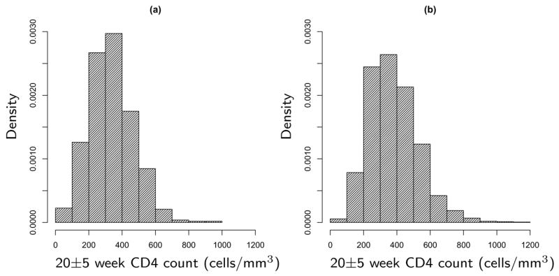
Histograms of CD4 counts at 20 ± 5 weeks: (a) ZDV monotherapy group. (b) Combined treatment group.

Table I shows results for estimation of β using several methods, including the unadjusted estimator Ȳ⁽¹⁾ − Ȳ⁽⁰⁾ and; because one of the baseline covariates is CD4 count, the usual estimator based on “change scores,” ${\overline{Y}}^{(1)}-{\overline{Y}}^{(0)}-({\overline{X}}_{CD4}^{(1)}-{\overline{X}}_{CD4}^{(0)})$, where ${\overline{X}}_{CD4}^{(k)}$ is mean baseline CD4 count in group k = 0, 1, which, using (15), may be written in the form (5). Also presented are β̂_{ANCOV A}, β̂_KOCH, and two versions of the proposed estimator β̂. For the latter, to develop the models for E(Y |Z = k, X), k = 0, 1, we used forward selection as a representative model selection approach available in standard software. For “Forward-1,” the models were developed separately by forward selection with entry criterion 0.05 allowing linear additive terms in elements of X. For “Forward-2”, the models were developed separately by forward selection allowing linear, quadratic, and two-way interaction terms in elements of X. We also used backward selection or different selection methods for each group, with similar results (not reported). Standard errors for the unadjusted and change score estimators were calculated via the usual formulæ; for β̂_{ANCOV A1} using both (18) and the least squares formula based on the fit of (3), as would ordinarily be the case in practice (indicated by *); and for β̂_KOCH and Forward-1 and -2 using (18).

Table I.

Estimates of β for the ACTG 175 data. Unadjusted is Ȳ⁽¹⁾−Ȳ⁽⁰⁾; Change scores is Ȳ⁽¹⁾−Ȳ⁽⁰⁾ − the difference in sample mean baseline CD4; Forward-1 is β̂ in (17) with treatment-specific regression models developed using forward selection allowing linear terms only in elements of X; Forward-2 is the same but allowing linear, quadratic, and two-way interaction terms; ANCOVA is β̂_{ANCOV A1} using all elements of X; and Koch is β̂_KOCH using all elements of X. SE is estimated standard error calculated as described in the text. Test Stat. is the Wald test statistic; and Rel. Eff. is (SE for the Unadjusted estimator)² divided by (SE for the indicated estimator)².

Estimator	Estimate	SE	Test Stat.	Rel. Eff.
Unadjusted	46.811	6.760	6.924	1.00
Change scores	50.409	5.509	9.150	1.51
Forward-1	49.896	5.135	9.716	1.73
Forward-2	51.139	5.103	10.021	1.75
ANCOVA	49.694	5.154	9.643	1.72
	–	5.647	8.799	1.43*
Koch	49.758	5.139	9.682	1.73

^*Row calculated using usual least squares SE

All methods indicate strong evidence of a treatment difference. All estimates are very similar with the exception of the unadjusted estimate, which is slightly lower due to a mild imbalance for baseline CD4 between groups. Baseline CD4 exhibits moderate association with CD4 at 20 ± 5 weeks, with correlation coefficients of roughly 0.6 in each treatment and a hint of curvature in the relationships; see Figure 1 of Reference [14]. Failure of the unadjusted estimator to take this relationship into account results in a much larger standard error than those of the other estimators; moreover, although the change score estimator offers substantial improvement, inclusion of additional covariate information yields further gains in precision. The proposed estimator with forward selection on linear terms and β̂_KOCH are virtually identical; allowing second-order effects to enter in the forward selection for the treatment-specific regression models for β̂ leads to very little additional reduction in estimated sampling variation; the resulting models include the square of baseline CD4, but because this effect is so mild, little gain is realized. Interestingly, the usual least squares standard error for β̂_{ANCOV A1} is noticeably larger than that based on (18); we discuss this in the next section.

The fitted treatment-specific models selected by “Forward-2” are, in obvious notation,

$$\begin{array}{l}E(Y|Z=0,X)\approx -79.705+1.599(\text{CD}4)-0.0007{(\text{CD}4)}^2-0.107(\text{CD}4\times \text{HEMO})\\ -0.005(\text{CD}4\times \text{WT})+0.013(\text{WT}\times \text{KARN})-0.040(\text{CD}8\times \text{HIST})-23.199(\text{HOMO}\times \text{RACE})\end{array}$$ (20)

$$\begin{array}{l}E(Y|Z=1,X)\approx 95.445+1.100(\text{CD}4)-0.0005{(\text{CD}4)}^2-142.288(\text{HOMO})\\ -0.178(\text{CD}4\times \text{DRUG})-0.087(\text{CD}4\times \text{RACE})+0.033(\text{CD}8\times \text{HEMO})-0.014(\text{CD}8\times \text{HOMO})\\ -0.021(\text{CD}8\times \text{HIST})-0.720(\text{AGE}\times \text{HIST})-0.554(\text{AGE}\times \text{SYMP})-0.706(\text{WT}\times \text{HEMO})\\ +1.282(\text{WT}\times \text{DRUG})+1.688(\text{KARN}\times \text{HOMO})-28.321(\text{DRUG}\times \text{RACE})\\ -45.337(\text{DRUG}\times \text{SEX})+35.981(\text{DRUG}\times \text{HIST})+24.032(\text{RACE}\times \text{HIST})-3.602(\text{SEX}\times \text{HIST}),\end{array}$$ (21)

with treatment-specific variance estimates var(Y |Z = 0, X) ≈ (95.82)² and var(Y |Z = 1, X) ≈ (115.63)², and coefficients of determination R² = 0.50 and 0.38.

It is important to recognize that we are uninterested in the interpretation of models (20) and (21). What is important is that they represent functions of X yielding predictions that come as close as possible to the values of the true treatment-specific regressions at the X_i. Thus, that these models do not, for example, include all main effect terms involving variables in the interaction terms is of no consequence for the purpose of estimating β.

6. SIMULATION STUDIES

We report on several simulation studies to demonstrate the performance of the proposed methods, each involving 5000 Monte Carlo data sets.

We consider first estimation of β under two scenarios. The initial scenario is based on the fit of the ACTG 175 data in Section 5. For each simulated data set, we generated for each of n subjects the continuous baseline covariates CD4 count, CD8 count, age, weight, and Karnofsky score from a multivariate normal distribution with the empirical mean and covariance matrix of these variables in the data. Independently, baseline binary indicators for hemophilia, homosexual activity, history of drug use, race, gender, antiretroviral history, and symptomatic status were generated for each subject from independent Bernoulli distributions using the observed data proportions for each. Treatment indicator Z was generated from Bernoulli(δ) for each subject, independently of all other variables. Finally, CD4 count at 20±5 weeks for each subject was generated from a normal distribution with conditional mean (20) or (21) and conditional variance given after (21) depending on his/her treatment assignment and covariates. The true value of β = 54.203, with R² = 0.50 and 0.39 for the treatment-specific regressions for k = 0, 1, consistent with the data. For each data set, β and standard errors were estimated using all methods in Table I. We also estimated β using (17), but with f̂_k,i for each i equal to the predicted values obtained from fitting the true forms of E(Y |Z = k, X), k = 0, 1, to the data, with standard errors obtained from (18). This serves as a “benchmark” achieving the smallest possible asymptotic variance in class (5).

Table II shows results for two instances of this scenario: n = 2139 and δ = 0.75, as in ACTG 175; and n = 400 and δ = 0.5, representing a moderate-sized trial with the 1:1 randomization common in practice. As all estimators showed negligible bias, bias is not reported. For both cases, any form of adjustment yields considerable efficiency gain over the unadjusted estimator. Improvement over simple adjustment based on change scores is achieved by incorporating additional covariates. The proposed method, β̂_{ANCOV A1}, and β̂_KOCH show similar precision, likely because baseline CD4 has a strong linear but only mild quadratic relationship with outcome, and other, weaker covariate relationships are captured adequately by main effect terms in all estimators, a view supported by the results for the “Benchmark” estimator, which shows little additional gain in efficiency. All methods except ANCOVA using least squares standard errors, shown for n = 2139, δ = 0.75, yield confidence intervals attaining the nominal coverage; see below. A key message is that the proposed method, represented here by “Forward-1” and “Forward-2,” allows analysts latitude to explore and exploit relationships in the data to come as close as possible to the “benchmark” gain in efficiency independently of reference to the treatment effect while attaining nominal operating characteristics.

Table II.

Results for the simulation scenario based on the ACTG 175 data using 5000 Monte Carlo data sets. Estimators are as in Table I; Benchmark is the proposed estimator found by fitting the true treatment-specific regressions to obtain predicted values. MC SD is Monte Carlo standard deviation, Ave SE is the average of standard error estimates, Cov. Prob. is coverage probability of a 95% Wald confidence interval, and Rel. Eff. is the Monte Carlo mean square error for the Unadjusted estimator divided by that for the indicated estimator.

Estimator	MC SE	Ave SE	Cov. Prob.	Rel. Eff.
n = 2139, δ = 0.75
Unadjusted	6.949	6.905	0.950	1.00
Change scores	5.570	5.529	0.947	1.55
Forward-1	5.229	5.156	0.943	1.77
Forward-2	5.177	5.075	0.943	1.80
ANCOVA	5.227	5.183	0.946	1.77
	–	5.657	0.965*	–
Koch	5.220	5.154	0.946	1.77
Benchmark	5.122	5.089	0.949	1.84
n = 400, δ = 0.5
Unadjusted	14.027	14.138	0.952	1.00
Change scores	11.485	11.560	0.952	1.49
Forward-1	10.927	10.850	0.951	1.65
Forward-2	10.975	10.680	0.945	1.64
ANCOVA	10.942	10.984	0.954	1.64
Koch	10.948	10.818	0.950	1.64
Benchmark	10.886	10.855	0.951	1.66

^*Row calculated using usual least squares SE

To emphasize this, we considered a second scenario identical to the first except that a stronger quadratic effect in baseline CD4 was introduced in the true E(Y |Z = k, X), k = 0, 1, while maintaining R² for these relationships at 0.50 and 0.39, and β = 54.203. This was accomplished by replacing the first three terms in (20) by −247.074+2.850(CD4)−0.0026(CD4)² and those in (21) by −82.931+2.400(CD4)−0.0025(CD4)². Table III shows results for n = 400, δ = 0.5. “Forward-1,” which considers only linear terms in elements of X; β̂_{ANCOV A1}; and β̂_KOCH all lead to similar gains over the unadjusted and change score estimators and, except for ANCOVA, admit confidence intervals achieving nominal coverage. “Forward-2,” which can incorporate the quadratic effect of baseline CD4, yields a noteworthy efficiency further gain.

Table III.

Results for the second simulation scenario data using 5000 Monte Carlo data sets. All entries are as in Table II.

Estimator	MC SE	Ave SE	Cov. Prob.	Rel. Eff.
n = 400, δ = 0.5
Unadjusted	14.084	14.148	0.951	1.00
Change scores	12.993	13.043	0.952	1.17
Forward-1	12.064	11.921	0.950	1.36
Forward-2	11.005	10.685	0.943	1.64
ANCOVA	12.076	12.068	0.952	1.36
Koch	12.081	11.892	0.949	1.36
Benchmark	10.885	10.853	0.951	1.67

As noted above, confidence intervals based on β̂_{ANCOV A1} and the usual standard errors obtained from the output of the least squares fit of (3) achieve Monte Carlo coverage exceeding the nominal level in Table II. Comparison of the average of these estimated least squares standard errors to the Monte Carlo standard deviation shows that this is because the former tends to overstate the true sampling variation. If the ANCOVA model (3) is a correct representation of E(Y |Z, X), and if in truth var(Y |Z, X) is constant, then the least squares standard errors will be consistent for the true sampling standard deviation of β̂_{ANCOV A1}. However, if these assumptions are violated, then this need not be the case; indeed, these assumptions do not hold in our simulation scenarios. Valid standard errors and nominal coverage may be obtained using the “sandwich” formula (18), as shown in Tables II and III, because (18) is not predicated on these assumptions. Thus, if ANCOVA is the basis for adjustment, as is widely proposed, least squares standard errors should not be used in general.

For each of the two scenarios with n = 400, δ = 0.5, we modified the intercept term in the true relationships E(Y |Z = k, X), k = 0, 1, so that the true value of β = 0, 15, and 30, and for each value of β we report in Table IV the proportion of 5000 Monte Carlo data sets for which a Wald test based on each estimator in Tables II and III rejected the null hypothesis β = 0 in favor of the one-sided alternative β > 0, where all tests were carried out at significance level 0.025. All tests exhibit the nominal level under the null hypothesis; under alternatives, the proposed methods achieve the highest power in both scenarios, notably in scenario 2.

Table IV.

Proportion of 5000 Monte Carlo data sets for which the null hypothesis β = 0 is rejected in favor of the alternative β > 0 using the test statistic based on each estimator and level of significance 0.025. Each of the two simulation scenarios in the text is considered with n = 400, δ = 0.50, and the intercept of the true E(Ȳ |Z = k, X), k = 0, 1, adjusted so that the true value of β is that indicated.

	Scenario 1			Scenario 2
Estimator	β = 0	β = 15	β = 30	β = 0	β = 15	β = 30
Unadjusted	0.027	0.183	0.567	0.027	0.183	0.569
Change scores	0.024	0.261	0.741	0.022	0.216	0.637
Forward-1	0.024	0.287	0.788	0.026	0.253	0.710
Forward-2	0.027	0.302	0.796	0.027	0.305	0.794
ANCOVA	0.023	0.281	0.782	0.024	0.240	0.699
Koch	0.025	0.293	0.791	0.026	0.249	0.707
Benchmark	0.025	0.290	0.790	0.025	0.290	0.790

As in any regression modeling context, there may be uncertainty associated with model development tasks for the f_k, including use of variable selection techniques such as forward selection, that is not taken into account by usual standard error formulæ [29]. We advocate the proposed methods when n is moderate-to-large, where our simulations, including those here, show that, for inference on β̂, these effects are negligible. For smaller n, a “correction” to (18) for model selection may be warranted [29]. It is natural to consider a nonparametric bootstrap [30] to obtain standard errors; however, whether this is theoretically justified is not established to our knowledge. With this caveat, we describe in the Appendix how use of the bootstrap would be possible in the principled framework in Section 4. We are studying methods for “correcting” standard errors for model selection and will report on this elsewhere.

7. DISCUSSION

We have demonstrated that systematic consideration of the covariate adjustment problem from the perspective of semiparametric theory leads to characterization of all consistent and asymptotically normal estimators for the treatment mean difference. Properties of familiar estimators and correspondences among them may be established and the most precise estimator identified. The results suggest methods for principled analysis, where adjustment for covariate effects is carried out separately from estimation of the treatment effect.

The decision on whether to propose a covariate-adjusted analysis during trial planning must weigh possible benefits relative to the increased effort involved [3]. Our proposed strategy involves logistical and cost considerations, and whether these are worthwhile must be determined in the particular context. Associations among covariates must be sufficiently strong for adjustment to pay off, and such covariates may not always be available. When adjustment is deemed potentially fruitful, our proposed approach may offer practical resolution to the conflict over whether and how to exploit covariate information to enhance efficiency.

We have focused on parametric modeling of the treatment-specific regressions. One may wonder if it is possible to use nonparametric approaches such as generalized additive models [31] or other multivariate smoothing methods to estimate these regressions; these may be prohibitive with more than a few covariates. As discussed by Leon et al. [14, sec. 4], because nonparametric estimators typically have large sample properties different from those of parametric estimators, such smoothing methods may be viable only in very large studies.

The methods presented in this article may be modified to accommodate outcome missing at random as shown in Davidian et al. [15]. As in the full data case considered here, models associated with both covariate adjustment and accounting for missing outcomes may be postulated and fitted independently of reference to the treatment effect, again supporting a principled analysis. Via application of semiparametric theory, the techniques for comparing two treatment means presented in this article may be extended to general measures of treatment effect, such as an odds ratio associated with a binary outcome, a hazards ratio associated with a censored time-to-event outcome, and so on, including accommodation of missing outcome and covariate information. We report on these developments elsewhere.

APPENDIX

In this appendix, we sketch arguments supporting assertions made in the main text. Consistency of estimators in (5). Ȳ⁽¹⁾−Ȳ⁽⁰⁾ is consistent for β; by Slutsky’s theorem, (5) itself is consistent for β if its second term $\stackrel{p}{\to }$ 0. Because $n_1/n\stackrel{p}{\to }\delta$, the second term is approximately equal to $n^{-1}{\sum }_{i=1}^n(Z_i-\delta )\{{(1-\delta )}^{-1}{h}^{(0)}(X_i)+{\delta }^{-1}{h}^{(1)}(X_i)\}\stackrel{p}{\to }E[(Z-\delta )\{{(1-\delta )}^{-1}{h}^{(0)}(X)+{\delta }^{-1}{h}^{(1)}(X)\}]=0$ because Z ⫫ X.

Asymptotic equivalence of β̂_{ANCOV A1} to (5) with h(k), k = 0, 1, as in (6). Straightforward algebra shows that the least squares estimator for β_Z in (3) is

$${\left\{1-\frac{n^2}{n_0{n}_1}{(n^{-1}{d}_1)}^T{\widehat{\mathrm{\sum }}}_{XX}^{-1}(n^{-1}{d}_1)\right\}}^{-1}\{{\overline{Y}}^{(1)}-{\overline{Y}}^{(0)}-\frac{n}{n_0{n}_1}\sum _{i=1}^n(Z_i-\overline{Z}){\widehat{\mathrm{\sum }}}_{XY}^T{\widehat{\mathrm{\sum }}}_{XX}^{-1}{X}_i\},$$ (A.1)

where $d_1={\sum }_{i=1}^n(Z_i-\overline{Z})X_i,{\widehat{\mathrm{\sum }}}_{XY}=n^{-1}{\sum }_{i=1}^n(X_i-\overline{X})(Y_i-\overline{Y})$, and ${\widehat{\mathrm{\sum }}}_{XX}=n^{-1}{\sum }_{i=1}^n(X_i-\overline{X}){(X_i-\overline{X})}^T$. Because Σ̂_XY and Σ̂_{XX $\stackrel{p}{\to }$} to their counterparts in (7), $n^2/(n_0{n}_1)\stackrel{p}{\to }{\{\delta (1-\delta )\}}^{-1}$, and $n^{-1}{d}_1\stackrel{p}{\to }0$, the first term in (A.1) is asymptotically equivalent to 1, while the second term is equivalent to (5) with h^(k), k = 0, 1 as in (6), yielding the result.

Asymptotic equivalence of β̂_{ANCOV A2} to (5) with h(k), k = 0, 1, as in (11), and to β̂_KOCH. The least squares estimator for β_Z in (10), obtained as described after (10), is

$${\left\{1-\frac{n^2}{n_0{n}_1}{(n^{-1}{d}_2)}^T{D}^{-1}(n^{-1}{d}_2)\right\}}^{-1}\left\{{\overline{Y}}^{(1)}-{\overline{Y}}^{(0)}-\frac{n}{n_0{n}_1}{d}_2^T{D}^{-1}\left(\begin{array}{c}{\widehat{\mathrm{\sum }}}_{XY}\\ {\widehat{\mathrm{\sum }}}_{\mathit{XYZ}}\end{array}\right)\right\},$$ (A.2)

where $d_2={\{d_1^T,{\sum }_{i=1}^n{(Z_i-\overline{Z})}^2{(X_i-\overline{X})}^T\}}^T,{\widehat{\mathrm{\sum }}}_{\mathit{XYZ}}=n^{-1}{\sum }_{i=1}^n(X_i-\overline{X})(Y_i-\overline{Y})(Z_i-\overline{Z})$, and

$$D=\left(\begin{array}{cc}{\widehat{\mathrm{\sum }}}_{XX}^{(0)}& {\widehat{\mathrm{\sum }}}_{XX}^{(1)}\\ {\widehat{\mathrm{\sum }}}_{XX}^{(1)}& {\widehat{\mathrm{\sum }}}_{XX}^{(2)}\end{array}\right),{\widehat{\mathrm{\sum }}}_{XX}^{(\ell )}=n^{-1}\sum _{i=1}^n{(Z_i-\overline{Z})}^{\ell }(X_i-\overline{X}){(X_i-\overline{X})}^T,$$

so ${\widehat{\mathrm{\sum }}}_{XX}^{(0)}={\widehat{\mathrm{\sum }}}_{XX}$. Clearly, D $\stackrel{p}{\to }$ block diag{Σ_XX, δ(1 − δ) Σ_XX}, and $n^{-1}{d}_2\stackrel{p}{\to }0$ (using randomization), so that, with $n^2/(n_0{n}_1)\stackrel{p}{\to }{\{\delta (1-\delta )\}}^{-1}$, the first term in (A.2) is asymptotically equivalent to 1. Because ${\sum }_{i=1}^n{(Z_i-\overline{Z})}^2(X_i-\overline{X})={\sum }_{i=1}^n(Z_i-\overline{Z})X_i(1-2\overline{Z}),\overline{Z}\stackrel{p}{\to }\delta ,{\widehat{\mathrm{\sum }}}_{XY}\stackrel{p}{\to }{\mathrm{\sum }}_{XY}=(1-\delta ){\mathrm{\sum }}_{XY}^{(0)}+\delta {\mathrm{\sum }}_{XY}^{(1)}$, and ${\widehat{\mathrm{\sum }}}_{\mathit{XYZ}}\stackrel{p}{\to }\delta (1-\delta )({\mathrm{\sum }}_{XY}^{(1)}-{\mathrm{\sum }}_{XY}^{(0)})$, we have after algebra for large n that

$$\begin{array}{l}{d}_2^T{D}^{-1}\left(\begin{array}{c}{\widehat{\mathrm{\sum }}}_{XY}\\ {\widehat{\mathrm{\sum }}}_{\mathit{XYZ}}\end{array}\right)\approx \sum _{i=1}^n(Z_i-\overline{Z}){[{\widehat{\mathrm{\sum }}}_{XY}+(1-2\delta ){\widehat{\mathrm{\sum }}}_{\mathit{XYZ}}/\{\delta (1-\delta )\}]}^T{\mathrm{\sum }}_{XX}^{-1}{X}_i\\ \approx \sum _{i=1}^n(Z_i-\overline{Z}){\{\delta {\mathrm{\sum }}_{XY}^{(0)}+(1-\delta ){\mathrm{\sum }}_{XY}^{(1)}\}}^T{\mathrm{\sum }}_{XX}^{-1}{X}_i,\end{array}$$ (A.3)

as required. To show the equivalence of β̂_KOCH to β̂_{ANCOV A2}, we show that the second term in (12), $V_{XY}^T{V}_{XX}^{-1}({\overline{X}}^{(1)}-{\overline{X}}^{(0)})$, can be written as n/(n₀n₁)×(A.3), where V_XY and V_XX are defined in (13). Because of (15), it suffices to find the limit in probability of $n{V}_{XY}^T{(n{V}_{XX})}^{-1}$. It is straightforward to show that, for large n, $n{V}_{XX}\approx {\delta }^{-2}{n}^{-1}{\sum }_{i=1}^n{Z}_i(X_i-{\overline{X}}^{(1)}){(X_i-{\overline{X}}^{(1)})}^T+{(1-\delta )}^{-2}{n}^{-1}{\sum }_{i=1}^n(1-Z_i)(X_i-{\overline{X}}^{(0)}){(X_i-{\overline{X}}^{(0)})}^T$, and $n{V}_{XY}\approx {\delta }^{-2}{n}^{-1}{\sum }_{i=1}^n{Z}_i(X_i-{\overline{X}}^{(1)})Y_i+{(1-\delta )}^{-2}{n}^{-1}{\sum }_{i=1}^n(1-Z_i)(X_i-{\overline{X}}^{(0)})Y_i$. Because by randomization $\overline{X}-{\overline{X}}^{(k)}\stackrel{p}{\to }0$, k = 0, 1, we may replace X̄^(k), k = 0, 1, by X̄ in these expressions, from whence $n{V}_{XX}\stackrel{p}{\to }{\{\delta (1-\delta )\}}^{-1}{\mathrm{\sum }}_{XX}$ and $n{V}_{XY}\stackrel{p}{\to }{\{\delta (1-\delta )\}}^{-1}\{(1-\delta ){\mathrm{\sum }}_{XY}^{(1)}+\delta {\mathrm{\sum }}_{XY}^{(0)}\}$, and the result follows.

Variance of β̂_{ANCOV A2}

We show that β̂_{ANCOV A2} has smallest asymptotic variance among all estimators of form (5) with h^(k), k = 0, 1, linear in X_i; i.e., $h^{(k)}(X_i)={\alpha }_{0k}+{\alpha }_k^T{X}_i$, say. It is straightforward to show that all such estimators satisfy

$$\begin{array}{l}{n}^{1/2}(\widehat{\beta }-\beta )=n^{1/2}({\overline{Y}}^{(1)}-{\overline{Y}}^{(0)}-\beta )-n^{-1/2}\sum _{i=1}^n(Z_i-\overline{Z})\left(\frac{n{\alpha }_0^T}{n_0}+\frac{n{\alpha }_1^T}{n_1}\right)X_i\\ \approx n^{-1/2}\sum _{i=1}^n\left(\left\{\frac{Z_i}{\delta }-\frac{1-Z_i}{1-\delta }\right\}{Y}_i-\beta -\frac{(Z_i-\delta )}{\delta (1-\delta )}[{\eta }_0+{\eta }^T\{X_i-E(X)\}]\right),\end{array}$$ (A.4)

where η₀ = δE(Y |Z = 0) + (1 − δ)E(Y |Z = 1), and η = δα₀ + (1 − δ)α₁. That with smallest variance takes η to minimize the variance of the summand in (A.4). The summand is A − η^T B, say. This is least squares problem [14, p. 1050], which yields ${\eta }^T=cov(A,B){\{var{(B)}^T\}}^{-1}={\{\delta {\mathrm{\sum }}_{XY}^{(0)}+(1-\delta ){\mathrm{\sum }}_{XY}^{(1)}\}}^T{\mathrm{\sum }}_{XX}^{-1}$. Comparing to (11), the result follows.

Demonstration of (16)

Similar to (A.4), for arbitrary h^(k), k = 0, 1, it is straightforward to show that $n^{1/2}(\widehat{\beta }-\beta )\approx n^{-1/2}{\sum }_{i=1}^n\phi (Y_i,Z_i,X_i;h^0,h^{(1)})$, where

$$\phi (Y,Z,X;h^0,h^{(1)})=\left(\frac{Z}{\delta }-\frac{1-Z}{1-\delta }\right)Y-\beta -\frac{(Z-\delta )}{\delta (1-\delta )}\{{\eta }_0+\delta h_c^{(0)}(X)+(1-\delta )h_c^{(1)}(X)\},$$

where $h_c^{(k)}(X)=h^{(k)}(X)-E\{h^{(k)}(X)|Z=k\}$, k = 0, 1. As f(Y, Z, X; h⁰, h⁽¹⁾) has mean zero because Z ⫫ X, the choices of h^(k), k = 0, 1, leading to the smallest variance asymptotically are those minimizing E{f²(Y, Z, X; h⁽⁰⁾, h⁽¹⁾)}. Letting $h_{\mathit{opt}}^{(k)}(X)=E(Y|Z=k,X)$, k = 0, 1, for brevity and writing $g_{\mathit{opt}}(X;h^{(0)},h^{(1)})=[{\eta }_0+\delta \{h_c^{(0)}(X)-h_{\mathit{opt}}^{(0)}(x)\}+(1-\delta )\{h_c^{(1)}(X)-h_{\mathit{opt}}^{(1)}(X)\}]/\{\delta (1-\delta )\}$, for any h^(k), k = 0, 1, we have

$$\begin{array}{l}E\{{\phi }^2(Y,Z,X;h^{(0)},h^{(1)})\}=E{[\{\phi (Y,Z,X;h_{\mathit{opt}}^{(0)},h_{\mathit{opt}}^{(1)})\}-(Z-\delta )g_{\mathit{opt}}(X;h^{(0)},h^{(1)})\}}^2]\\ =E\{{\phi }^2(Y,Z,X;h_{\mathit{opt}}^{(0)},h_{\mathit{opt}}^{(1)})\}+\delta (1-\delta )E\{g_{\mathit{opt}}^2(X;h^{(0)},h^{(1)})\}\\ \ge E\{{\phi }^2(Y,Z,X;h_{\mathit{opt}}^{(0)},h_{\mathit{opt}}^{(1)})\}\end{array}$$ (A.5)

where (A.5) follows because Z ⫫ X implies that the crossproduct $E\{{\phi }^2(Y,Z,X;h_{\mathit{opt}}^0,h_{\mathit{opt}}^{(1)})(Z-\delta )g_{\mathit{opt}}(X;h^{(0)},h^{(1)})\}=0$, demonstrating (16). In fact, it is immediate from (A.5) that, by taking h^(k) = 0, k = 0, 1, $\text{Avar}(\widehat{\beta })=\text{Avar}({\overline{Y}}^{(1)}-{\overline{Y}}^{(0)})-\delta (1-\delta )E\{g_{\mathit{opt}}^2(X;0,0)\}$, where “Avar” denotes “asymptotic variance,” showing that using the optimal choices in (16) is guaranteed to lead to a reduction in variance over the unadjusted estimator.

By a similar argument, one may in fact show that, if one restricts attention to representations for h^(k)(X) that are linear in X; i.e., $h^{(k)}(X)={\alpha }_{0k}+{\alpha }_k^{T}X$, k = 0, 1, and fits this model by treatment-specific least squares, then the resulting estimator for β has asymptotic variance $\text{Avar}({\overline{Y}}^{(1)}-{\overline{Y}}^{(0)})-{\{\delta (1-\delta )\}}^{-1}{\{\delta {\mathrm{\sum }}_{XY}^{(0)}+(1-\delta ){\mathrm{\sum }}_{XY}^{(1)}\}}^T{\mathrm{\sum }}_{XX}^{-1}\{\delta {\mathrm{\sum }}_{XY}^{(0)}+(1-\delta ){\mathrm{\sum }}_{XY}^{(1)}\}$. This holds regardless of whether the true E(Y |Z = k, X) are linear. Thus, representing h^(k), k = 0, 1 by linear functions leads to a reduction in variance over Ȳ⁽¹⁾ − Ȳ⁽⁰⁾.

Effect of parameter estimation in postulated models for E(Y |Z = k, X), k = 0, 1. As in Section 4, suppose we specify regression models f_k(X_i, α_k) for E(Y | Z = k, X), k = 0, 1, and we fit the models by solving appropriate regression estimating equations to obtain estimators α̂_k. As an example, for continuous Y we may solve the least squares equations ${\sum }_{i=1}^n\{Y_i-f_k(X_i,{\alpha }_k)\}{f}_{k,\alpha }(X_i,{\alpha }_k)=0$, f_k,α(Xi, αk) = ∂/∂α_kf_k(X_i, α_k). Under regularity conditions, ${\widehat{\alpha }}_k-{\alpha }_k^{\ast }=O_p(n^{-1/2})$, where ${\alpha }_k^{\ast }$ satisfies ${\sum }_{i=1}^{n}E\{Y_i-f_k(X_i,{\alpha }_k^{\ast })\}{f}_{k,\alpha }(X_i,{\alpha }_k^{\ast })=0$ [32, sec. A.6.5], and similarly for other estimating equations. If f_k(X_i, α_k) is a correct model for E(Y |Z = k, X), then ${\alpha }_k^{\ast }$ is the value satisfying $E(Y|Z=k,X)=f_k(X,{\alpha }_k^{\ast })$; if not, ${\alpha }_k^{\ast }$ is still some constant value. Either way, β̂ satisfies

$$\begin{array}{l}{n}^{1/2}(\widehat{\beta }-\beta )=n^{1/2}({\overline{Y}}^{(1)}-{\overline{Y}}^{(0)}-\beta )-n^{-1/2}\sum _{i=1}^n(Z_i-\overline{Z})\left\{\frac{n}{n_0}{f}_0(X_i,{\widehat{\alpha }}_0)+\frac{n}{n_1}{f}_1(X_i,{\widehat{\alpha }}_1)\right\}\\ \approx n^{-1/2}\sum _{i=1}^n\left[\left\{\frac{Z_i}{\delta }-\frac{1-Z_i}{1-\delta }\right\}{Y}_i-\beta -\frac{(Z_i-\delta )}{\delta (1-\delta )}\{{\eta }_0+\delta f_0^c(X_i,{\alpha }_0^{\ast })+(1-\delta )f_1^c(X_i,{\alpha }_1^{\ast })\}\right]\end{array}$$ (A.6)

$$+\sum _{k=0}^1{\delta }^{-k}{(1-\delta )}^{k-1}\left\{n^{-1}\sum _{i=1}^n(Z_i-\delta )f_{k,\alpha }(X_i,{\alpha }_k^{\ast })\right\}{n}^{1/2}({\widehat{\alpha }}_k-{\alpha }_k^{\ast }),$$ (A.7)

where $f_k^c(X_i,{\alpha }_k^{\ast })=f_k(X_i,{\alpha }_k^{\ast })-E\{f_k(X_i,{\alpha }_k^{\ast })\}$, k = 0, 1. The term in (A.7) converges in probability to zero because Z ⫫ X. Thus, n^1/2(β̂ − β) has the same limit in distribution as (A.6), which depends on the $f_k(X,{\alpha }_k^{\ast })$, which are fully specified as functions of X given ${\alpha }_k^{\ast }$. The smallest achievable large sample variance is that of the limit in distribution of (A.6) when $f_k(X,{\alpha }_k^{\ast })=E(Y|Z=k,X)$, k = 0, 1; i.e., f_k coincide with the true regression relationships. Estimator for sampling variance of β̂. The summand in (A.6) is the form of the influence function [13] for the proposed estimator β̂. Applying the sandwich technique and replacing this summand by an empirical version yields the sum in (18). We take C = (n −1)/(n −p −1) for β̂_{ANCOV A1}; C = {(n₀ − pn₁/n − 1) − 1 + (n₁ − pn₀/n − 1) − 1}/{(n₀ − 1) − 1 + (n₁ − 1) − 1} for β̂_KOCH, which generalizes the correction proposed by Lesaffre and Koch when n₀ = n₁ [3]; and C = {(n₀ −p₀ −1) − 1 +(n₁ −p₁ −1) − 1}/{(n₀ −1) − 1 +(n₁ −1) − 1} for β̂, where p_k, k = 0, 1, are the number of parameters fitted in each model f_k, k = 0, 1, exclusive of intercepts.

To obtain an alternative estimator for the sampling variance using the bootstrap, at step (i) of Section 4, B bootstrap data sets could be obtained, each by resampling n subjects with replacement from the original data. Each could be partitioned into two sets, i.e., ${\mathcal{D}}_b^{(k)\ast }$, k = 0, 1 for b = 1, …, B. In step (ii) of Section 4, the modeling strategy used on the actual data ${\mathcal{D}}^{(k)}$ for each k would also be replicated by the analysts responsible for each ${\mathcal{D}}_b^{(k)\ast }$, b = 1, …, B. The fitted model so obtained for each B = 1, …, B, f_k,b(X, α̂_k,b), say, could be reported along with the model developed for the actual data. In step (iii), predicted values for each k and bootstrap data set could then be constructed and used with ${\mathcal{D}}_b^{(k)\ast }$, k = 0, 1, B = 1, …, B, to construct B bootstrap estimates β̂_b, B = 1, …, B, using (17). The estimated standard error for β̂ would then be obtained as the square root of the sample variance of the β̂_b, B = 1, …, B.

References

- 1.Pocock SJ, Assmann SE, Enos LE, Kasten LE. Subgroup analysis, covariate adjustment and baseline comparisons in clinical trial reporting: current practice and problems. Statistics in Medicine. 2002;21:2917–2930. doi: 10.1002/sim.1296. [DOI] [PubMed] [Google Scholar]
- 2.Koch GG, Tangen CM, Jung JW, Amara IA. Issues for covariance analysis of dichotomous and ordered categorical data from randomized clinical trials and non-parametric strategies for addressing them. Statistics in Medicine. 1998;17:1863–1892. doi: 10.1002/(sici)1097-0258(19980815/30)17:15/16<1863::aid-sim989>3.0.co;2-m. [DOI] [PubMed] [Google Scholar]
- 3.Lesaffre E, Bogaerts K, Li X, Bluhmki E. On the variability of covariance adjustment: experience with Koch’s method for evaluating the absolute difference in proportions in randomized clinical trials. Controlled Clinical Trials. 2002;23:127–142. doi: 10.1016/s0197-2456(01)00201-x. [DOI] [PubMed] [Google Scholar]
- 4.Lesaffre E, Senn S. A note on non-parametric ANCOVA for covariate adjustment in randomized clinical trials. Statistics in Medicine. 2003;22:3586–3596. doi: 10.1002/sim.1583. [DOI] [PubMed] [Google Scholar]
- 5.Senn S. Covariate imbalance and random allocation in clinical trials. Statistics in Medicine. 1989;8:467–475. doi: 10.1002/sim.4780080410. [DOI] [PubMed] [Google Scholar]
- 6.Altman DG. Adjustment for covariate imbalance. In: Armitage P, Colton T, editors. Encyclopedia of Biostatistics. 2. Wiley: Chichester; 2005. pp. 1273–1278. [Google Scholar]
- 7.Assmann SF, Pocock SJ, Enos LE, Kasten LE. Subgroup analysis and other (mis)uses of baseline data in clinical trials. The Lancet. 2000;355:1064–1069. doi: 10.1016/S0140-6736(00)02039-0. [DOI] [PubMed] [Google Scholar]
- 8.Raab GM, Day S, Sales J. How to select covariates to include in the analysis of a clinical trial. Controlled Clinical Trials. 2000;21:330–342. doi: 10.1016/s0197-2456(00)00061-1. [DOI] [PubMed] [Google Scholar]
- 9.Senn S. Consensus and controversy in pharmaceutical statistics. The Statistician. 2000;49:135–176. [Google Scholar]
- 10.Lewis JA. Statistical principles for clinical trials (ICH E9): an introductory note on an international guideline. Statistics in Medicine. 1999;18:1903–1904. doi: 10.1002/(sici)1097-0258(19990815)18:15<1903::aid-sim188>3.0.co;2-f. [DOI] [PubMed] [Google Scholar]
- 11.Grouin JM, Day S, Lewis J. Adjustment for baseline covariates: an introductory note. Statistics in Medicine. 2004;23:697–699. doi: 10.1002/sim.1646. [DOI] [PubMed] [Google Scholar]
- 12.Hauck WW, Anderson S, Marcus SM. Should we adjust for covariates in nonlinear regression analyses of randomized trials? Controlled Clinical Trials. 1998;19:249–256. doi: 10.1016/s0197-2456(97)00147-5. [DOI] [PubMed] [Google Scholar]
- 13.Tsiatis AA. Semiparametric Theory and Missing Data. Springer; New York: 2006. [Google Scholar]
- 14.Leon S, Tsiatis AA, Davidian M. Semiparametric estimation of treatment effect in a pretest-posttest study. Biometrics. 2003;59:1048–1057. doi: 10.1111/j.0006-341x.2003.00120.x. [DOI] [PubMed] [Google Scholar]
- 15.Davidian M, Tsiatis AA, Leon S. Semiparametric estimation of treatment effect in a pretest-posttest study with missing data (with Discussion) Statistical Science. 2005;20:261–301. doi: 10.1214/088342305000000151. [DOI] [PMC free article] [PubMed] [Google Scholar]
- 16.Robins JM, Rotnitzky A, Zhao LP. Estimation of regression coefficients when some regressors are not always observed. Journal of the American Statistical Association. 1994;89:846–866. [Google Scholar]
- 17.Robins JM. ASA Proceedings of the Bayesian Statistical Science Section. American Statistical Association; Alexandria, Virginia: 2000. Robust estimation in sequentially ignorable missing data and causal inference models; pp. 6–10. [Google Scholar]
- 18.Cassel CM, Sarndal CE, Wretman JH. Some results on generalized difference estimation and generalized regression estimation for finite populations. Biometrika. 1976;63:615–620. [Google Scholar]
- 19.Cochran WG. Sampling Techniques. 3. Wiley; New York: 1977. [Google Scholar]
- 20.Sarndal CE, Swensson B, Wretman J. Model Assisted Survey Sampling. Springer; New York: 1992. [Google Scholar]
- 21.Yang L, Tsiatis AA. Efficiency study for a treatment effect in a pretest-posttest trial. The American Statistician. 2001;55:314–321. [Google Scholar]
- 22.Korsholm L, Vach W. Covariate adjustment in clinical trials - A semiparametric view (meeting abstract 41) Controlled Clinical Trials. 2003;24:62S–63S. [Google Scholar]
- 23.Stefanski LA, Boos DD. The calculus of M-estimation. The American Statistician. 2002;56:29–38. [Google Scholar]
- 24.Tibshirani R. Regression shrinkage and selection via the Lasso. Journal of the Royal Statistical Society, Series B. 1996;58:267–288. [Google Scholar]
- 25.Fan J, Li R. Variable selection via nonconcave penalized likelihood and its oracle property. Journal of the American Statistical Association. 2001;96:1348–1360. [Google Scholar]
- 26.Wu T, Boos DD, Stefanski LA. Controlling variable selection by the addition of pseudo variables. Journal of the American Statistical Association. 2007;102:235–243. [Google Scholar]
- 27.Harrell FE. Regression Modeling Strategies, With Applications to Linear Models, Logistic Regression, and Survival Analysis. Springer; New York: 2001. [Google Scholar]
- 28.Hammer SM, Katzenstein DA, Hughes MD, Gundaker H, Schooley RT, Haubrich RH, Henry WK, Lederman MM, Phair JP, Niu M, Hirsch MS, Merigan TC for the AIDS Clinical Trials Group Study 175 Study Team. A trial comparing nucleoside monotherapy with combination therapy in HIV-infected adults with CD4 cell counts from 200 to 500 per cubic millimeter. New England Journal of Medicine. 1996;335:1081–1089. doi: 10.1056/NEJM199610103351501. [DOI] [PubMed] [Google Scholar]
- 29.Shen X, Huang HC, Ye J. Inference after model selection. Journal of the American Statistical Association. 2004;99:751–762. [Google Scholar]
- 30.Brookhart MA, van der Laan MJ. A semiparametric model selection criterion with applications to the marginal structural model. Computational Statistics and Data Analysis. 2006;50:475–498. [Google Scholar]
- 31.Hastie TJ, Tibshirani RJ. Generalized Additive Models. Chapman and Hall; London: 1990. [Google Scholar]
- 32.Carroll RJ, Ruppert D, Stefanski LA, Crainiceanu CM. Measurement Error in Nonlinear Models: A Modern Perspective. 2. Chapman and Hall/CRC; New York: 2006. [Google Scholar]