A tree-based method for modeling a multivariate ordinal response

Abstract

Motivated by a real example of understanding the so-called “building related occupant complaint syndromes” (BROCS), we propose a tree-based method for analyzing a multivariate ordinal response. Our method is semiparametric by assuming a within-node parametric distribution on the adaptive nonparametric tree framework. We use simulation experiments to demonstrate the ability of our method to identify underlying structures in the data and the fact that analyzing ordinal response data with proper methods that take ordinality into account is considerably more powerful than dichotomization. The reanalysis of the BROCS data also suggests new insights that go beyond a previous analysis based on the dichotomization.

1. INTRODUCTION

In many studies such as health surveys, researchers collect information from multiple items or sources to determine the condition or disease status of a subject. For example, in a study of the so-called “building related occupant sick syndromes” (BROCS), responses on six clusters of complaints were collected from each of the 6,800 respondents. It is noteworthy that the choices for many items in the BROCS study are “never”, “rarely”, “sometimes”, “often”, and “always”, or a subset of these choices. To analyze such data, a common practice is to dichotomize the ordinal scaled responses by collapsing them into “yes” or “no” and then model the derived multivariate binary response as in Zhang (1998). While convenient, such a dichotomization is not ideal because it leads to loss of information and the decision of collapsing which levels into the same group is often subjective. We will demonstrate later that analyzing ordinal response data with proper methods that take ordinality into account is considerably more powerful than dichotomization.

In the past decade, it has become a very active research area to directly analyze ordinal responses instead of dichotomizing them first. Agresti (1999) provides a thorough review and extensive literature on some of the advances in this area. For example, Hedeker and Gibbons (1994) proposed a random-effect regression model for the analysis of multiple correlated ordinal responses. They assumed a linear regression model for latent unobserved continuous responses that underlie the observed ordinal responses. Then, either a cumulative probit or cumulative logit link function was used to model the response functions. Ten Have (1996) proposed a mixed effects model to analyze ordinal responses and derived a closed form for the marginal log-likelihood when the distribution of the random effects is log-gamma with the cumulative complementary log-log link function.

It is evident from Agresti (1999) and other work that random or mixed effects models are the basis of the parametric models for analyzing ordinal responses and that many useful models and approaches have been established. However, little progress has been made in using nonparametric techniques to deal with correlated ordinal responses, which can be particularly useful when the underlying structure in the data is not apparent and an exploratory step is desirable. In one exception, Kauermann (2000) introduced local smoothing in a regression model for clustered or longitudinal data with ordinal responses. In essence, the nonparametric technique is used to estimate the marginal parameters such as fixed effects and within-subject correlations. The main motivation for this work is to fill in this methodological gap.

Analyzing ordinal response data with proper methods that take ordinality into account is considerably more powerful than dichotomization (e.g., Zhang et al. 2003, Zhang et al. 2006). We mentioned a few different ways to analyze a multivariate ordinal response. In this paper, we develop a tree-based approach to the analysis of multivariate ordinal data, because it is an undeveloped area, and in many studies we have little information as to which and how predictors are related to the responses.

Like Zhang (1998) and Kauermann (2000), our approach is a hybrid of nonparametric and parametric methods, and is best termed as a semiparametric one. The idea is that the specific tree structure is not known and will be determined from the data – this is the nonparametric aspect of the method – and that whenever we have a tree, even temporarily, we assume a particular form of within-node distribution – this is the parametric aspect of the method. This idea has been frequently used in the development of tree-based methods (Zhang, 1998; Zhang and Singer 1999). Later, we will describe in detail what we mean by a node as well as other terminologies.

2. METHOD

2.1 The model

Assume that there are N units of observations in the data. Within unit i, we observe n ordinal responses denoted by z_i and p covariates denoted by x_i. In longitudinal studies, the set of responses within a unit results from repeated measures from the same subject, and the covariates may be constant in the unit or depend on the component of the unit, i.e., time varying. In other studies such as in Zhang (1998), the set of responses within a unit is comprised of different sites or symptoms of a disease, e.g., different sites of cancer, different respiratory symptoms, comorbid psychiatric diseases, and different substance abuses. Again, the covariates can be constant within the unit, or vary by the individual component of the unit. In this work, we only consider covariates that are common within the observation unit.

Let z_ij denote the jth ordinal response in the ith unit, and suppose that it takes a value from 1,…, K. For clarity and without loss of generality, the number of categories K is assumed to be the same for all response variables, because we can create extra levels with zero frequency when different responses have different numbers of categories. Let us define K − 1 indicator variables y_ijk = I (z_ij > k), for k = 1,…, K − 1. Here I(·) is the indicator function. Let

$$\begin{array}{rl}{y}_{ij}=& {(y_{ij,1},\dots ,y_{ij,K-1})}^{\text{T}},\\ y_i=& {(y_{i1}^{\text{T}},\dots ,y_{in}^{\text{T}})}^{\text{T}},\end{array}$$ (1)

Then, the observed responses from the ith unit can be rewritten as

$$y_i={(y_{i1,1},\dots ,y_{i1,K-1},\dots ,y_{in,1},\dots ,y_{in,K-1})}^{\text{T}},$$

and the covariates are

$$x_i={(x_{i1},\dots ,x_{ip})}^{\text{T}},$$

i = 1,…, N. Our objective is to characterize the distribution of y_i based on x_i.

2.2 Node-split criterion

As in the general tree methodology (Breiman et al. 1984 and Zhang and Singer 1999), the construction of a tree begins with splitting the root node that consists of all data in a learning sample. Once the root node is divided into two daughter nodes, we apply the same procedure to partition the daughter nodes. This process is referred to as the recursive partitioning procedure, and it is the thrust of the tree formation. Thus, in this section, we concentrate on splitting the root node into the left daughter(t_L) and right daughter(t_R).

For an ordered covariate (on an ordinal or continuous scale), say x_j, and a threshold value c, whether unit i is assigned to the left or right daughter node is based on the question whether or not x_ij > c. If x_j is a categorical covariate, the assignment is made according to a particular set of some levels that this covariate can take. All covariates and their splitting values together usually yield many ways of splitting the root node. Hence, a splitting criterion to select the best split is needed.

Following the approach of Zhang (1998) for handling multiple binary responses, we assume an intermediate within-node joint distribution of the responses within a unit. Precisely, for the ith unit, we consider a within-node joint distribution for z_i as follows

$$f_i(z_i;\psi ,\omega )=exp\{{\psi }^{\text{T}}{y}_i+{\omega }^{\text{T}}{w}_i-A_i(\psi ,\theta )\},$$ (2)

where ψ and ω are vectors of parameters, A_i(ψ, ω) is the normalization constant which is the summation over Kⁿ possible assignments for the value of z_i. Moreover, y_i is defined in (1) and

$$\begin{array}{ll}{w}_i=& (y_{i1,1}{y}_{i2,1},\dots ,y_{i1,1}{y}_{i2,(K-1)},\dots ,\\ & y_{i(n-1),(K-1)}{y}_{in,(K-1)}{)}^{\text{T}}.\end{array}$$ (3)

Because w_i consists of pairwise interactions between all indicators of two responses, its coefficient vector ω contains the information on the “correlation” of the two responses. In fact, in simple cases, these coefficients are odds ratios, which are commonly used to describe the association between two binary variables.

Without restrictions, ψ and ω have (K − 1)n and (K − 1)²n(n − 1)/2 elements, respectively. To reduce the number of the free parameters and retain the ordinality property of the responses, we introduce a link matrix C and let ω = Cθ, where

$$C={\mathbf{1}}_n\otimes I_{{(K-1)}^2}.$$ (4)

Here I_m denotes an m × m identity matrix for an integer m, 1_n is an n-vector of ones, and ⊗ refers to the operator for the Kronecker product. Then, the joint probability distribution of z_i becomes

$$f_i(z_i;\psi ,\theta )=exp\{{\psi }^{\prime }{y}_i+(C\theta {)}^{\prime }{w}_i-A_i(\psi ,\theta )\}.$$ (5)

Remark

The implication of this parameter reduction is to assume that the correlation structure among any two pair of responses is the same, but varies for different ordinal levels to retain the ordinality of the responses. We should note that the heterogeneity in different responses is reflected through the “prevalence” parameter ψ. In other words, the “prevalence” parameters depend on a specific response and its ordinal level while the “correlation” parameters are only functions of the ordinal level. Such assumptions may not be ideal, but are quite common in analysis of correlated data.

Once the within-node distribution is defined, the maximum log-likelihood can serve as a splitting criterion. That is, for any node t, we obtain

$$h(t)=\sum _{\{\text{unit }i\in t\}}\{{\widehat{\psi }}^{\prime }{y}_i+(C\widehat{\theta }{)}^{\prime }{w}_i-A_i(\widehat{\psi },\widehat{\theta })\},$$ (6)

where ψ̂ and θ̂ are the maximum likelihood estimators of ψ and θ based on samples in node t. Thus, we select a split from all allowable ones to maximize the sum of the generalized entropies, h(t_L)+h(t_R), from the resulting two daughter nodes. Because the pool of allowable splits is usually large and the assessment of each allowable split entails a maximization, we want to reduce the computational burden to its minimal level. In the appendix, we discuss in detail the computation issues.

In addition to the distribution assumed in (2), there are other alternative distributions that are commonly used in analysis of multivariate ordinal variables. For example, we considered a simple approach by treating the ordinal responses as numerical responses, and we will present simulation results from this approach below. In addition, we evaluated another approach based on the multivariate distribution of Hedeker and Gibbons (1994). This approach is computationally complicated and the resulting trees were not preferable according to our simulation (data are not presented here). On the basis of this empirical evidence, we adopted the exponential distribution in (2).

2.3 Tree pruning

So far, we have explained the recursive partitioning procedure for growing a tree. Because we do not employ any stopping procedure, the resulting tree is generally large and over grown. Thus, it is important to determine an appropriate size of the final tree for interpretation. This step is usually referred to as pruning. The commonly used procedures include error based pruning (Quinlan 1987, 1993), minimum error pruning (Niblett and Bratko 1986), critical value pruning (Mingers 1987), and cost-complexity pruning (Breiman 1984). Esposito et al. (1997) compared these pruning methods and found no clear winner. Later, Li et al. (2001) proposed a pruning method that combines dynamic programming and classical optimization technique. Here, we use the cost-complexity concept, because it can be easily generalized from a single response to multiple responses.

Briefly, we divide the entire sample into a number of groups (e.g., 2, 5 or 10) of approximately equal sizes. If we use a υ-fold cross validation, the original sample is randomly divided into υ groups. We repeat the tree growing procedure υ times, and each time we use υ −1 of the υ subgroups of the sample as the learning sample alternatively for tree growing and the left-over subgroup as the test sample to evaluate the predictive quality of the tree. The final tree is determined to optimize the predictive quality based on the cross-validation.

To determine the final tree, we follow the steps of Breiman et al. (1984). There are four preparation steps before cross validation is applied. First, we introduce a complexity parameter, α that is used to penalize a large tree. Secondly, let T̃ denote the set of all terminal nodes of a tree T. We define the cost for tree T, denoted by R(T), as

$$R(T)=-\sum _{t\in \stackrel{\sim }{T}}\sum _{\text{unit }i\in t}logf(y_i;\widehat{\mathrm{\Psi }},\widehat{\theta }),$$ (7)

where f is defined as in (5). Thirdly, we introduce a cost-complexity for a tree T as

$$R_{\alpha }(T)=R(T)+\alpha \mid \stackrel{\sim }{T}\mid ,$$ (8)

where |T̃| is the number of terminal nodes. Lastly, we can find an increasing sequence of complexity parameters,

$${\alpha }_0<{\alpha }_1<\cdots <{\alpha }_m,$$ (9)

each of which leads to a smallest subtree of T with the lowest cost. Here, α₀ = 0. It is important to note that the resulting sequence of subtrees is nested. That is, we have a sequence of nested optimal subtrees as follows:

$$T_0\supset T_1\supset \cdots \supset T_m,$$

where T₀ is the initial tree and corresponds to α₀ and T_n is the smallest tree containing the root node only.

Now, we are ready to select the final tree from the above sequence of optimal subtrees through cross validation. During the kth fold of the cross validation, we regrow a large tree, denoted by $T_0^{(k)}$ using the learning sample. Then, we apply the sequence of the complexity-parameters in (9) to produce a nested sequence of subtrees of $T_0^{(k)}$. We denote this sequence by

$$T_0^{(k)}\supseteq T_1^{(k)}\supseteq \cdots \supseteq T_m^{(k)}.$$

For each subtree $T_l^{(k)}$, we compute its cost, $R^{cv}(T_l^{(k)})$, as in (7) using the test sample, whereas Ψ̂ and θ̂ are fixed from the learning sample. The cross validation cost, R^cυ(T_l), of subtree T_l is the average of $R^{cv}(T_l^{(k)})$ over the υ folds. We can select the subtree with the smallest cross validation cost. However, as discussed in Breiman et al. (1984), it is sometimes helpful to consider the so-called one-standard error rule to overcome the instability of the subtree with the minimal cross validation cost. Instead of choosing the subtree T_s with the minimal cross validation cost, we choose the smallest subtree T_s1 such that

$$R^{cv}(T_{s_1})\le R^{cv}(T_s)+SE(R^{cv}(T_s)),$$ (10)

where SE(R^cυ (T_s)) is the standard error of R^cυ (T_s).

Theoretical estimation of SE(R^cυ (T_s)) is complex even in the simplest tree framework. Thus, we repeat the five-fold cross-validation process a number of times (e.g., 10) and obtain an estimate of SE(R^cυ (T_l)) for l = 0,…, m.

3. SIMULATION

In this section, we present simulation studies to evaluate the node-splitting measure, h(t), in (6). The data are simulated as follows. We included the same 22 covariates as in the real data set to be presented in Section 4. A latent continuous variable U underlying the observed ordinal variable Z was generated from the following model:

$$u_{ik}=b_i+0.5I(x_{15}>1)+1.0I(x_{13}>3)+0.5I(x_7>1)+{\epsilon }_{ik},$$ (11)

where b_i ~ N (0, 1) is the random intercept, ε_ik ~ N (0, 2) is the residual term, and they are all independent for k = 1,…, 6, i = 1,…, 6800. A 3-level ordinal response is determined by

$$z_{ik}=\{\begin{array}{ll}0\hfill & \text{if }{u}_{ik}\le 1,\hfill \\ 1\hfill & \text{if }{u}_{ik}\in (1,3],\hfill \\ 2\hfill & \text{if }{u}_{ik}>3.\hfill \end{array}$$

Thus, 19 of the 22 covariates were included in the dataset as noise variables. We should note that the data generating model is not in a tree structure.

To speed up the computation, we used a 2-fold cross-validation during the tree pruning, and replicated the cross-validation 10 times to obtain the standard error of the cross validation estimate of the tree cost. The simulation experiment was replicated 100 times.

The resulting trees correctly selected X₇ > 1, X₁₃ > 3, and X₁₅ > 1 as the splits in 96 of the 100 runs. X₁₃ > 3 is always the one to split the root node. In only 1 of the 100 runs, the tree included an additional split based on X₁₀ > 1. In only 3 of the 100 runs, the trees did not select X₁₅ > 1. Thus, the trees based on h(t) are highly sensitive and specific in revealing the true splits.

As mentioned earlier, we also evaluated alternative splitting criteria. For example, the simplest way is to treat the ordinal responses as numerical values and use the correlation matrix with each node as the basis for splitting. This criterion was studied by Segal (1992) and Zhang (1998). In 21 of the 100 runs, the final trees selected a noise variable. In six runs out of 100, the final trees had only one split, which was X₁₃ > 3. The other two variables were not used. Hence, treating the ordinal responses as if they were numerical is not a satisfactory approach.

To further evaluate the validity of our method, we performed additional simulations to investigate the ability of our proposed method in identifying the relevant splits when the data are generated from tree-based models. Although the real data are not likely to conform the exact tree structures, it is still useful to understand the performance of the trees under the hypothetical situations.

Our simulation data were generated from a tree with 3 layers and 4 terminal nodes as displayed in Figure 1. The units in the four terminal nodes had different joint probability distributions determined by the parameters (ψ₁₁, ψ₁₂, ψ₂₁,…, ψ₆₂, θ₁₁, θ₁₂, θ₂₁, θ₂₂). These parameters were set to (−1., −3., −1.4, −3., −1., −3.2, −1.2, −3., −1.4, −3.6, −1.4, −3.2, 0.5, 0.0, 0.4, 0.5); (−1., −3., −1.5, −3., −1., −3.2, −1.2, −3., −1.2, −3.2, −1.3, −3.1, 0.5, 0.4, 0.4, 0.5); (−1., −3.1, −0.9, −3., −1.1, −3.1, −1.0, −3.2, −1.0, −3.2, −1.0, −3.4, 0.5, 0.2, 0.4, 0.5); and (−1., −3.1, −1.0, −3., −1.4, −3.1, −1.0, −3., −1.1, −3.2, −1.0, −3.4, 0.5, 0., 0., 0.5) for nodes 4, 5, 6 and 7, respectively. Again, we used the same covariates as the real data set to be analyzed below, and 19 of the 22 covariates were included in the data sets as noise variables. Furthermore, we generated six 3-level ordinal responses.

Figure 1.

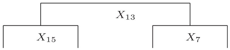
Predefined Tree Used in the Simulation.

We replicated our simulation 50 times. After pruning, 49 of the 50 final trees were exactly the same as in Figure 1. The lone missed one contained the three underlying splits, however. Thus, this simulation experiment validates our method.

If the goal is to identify relevant splits that are predictive of the responses, it is useful to know whether we can also achieve this goal by collapsing the three-level ordinal responses to two-level binary responses and applying the existing tree based method. For example, let us collapse the first two levels into the same one. Using the same 50 replications as described above, we constructed 50 trees using the multiple binary outcomes. Thirteen out of the 50 trees are the same as the underlying tree in Figure 1. Thirty trees out of 50 are of the same form as depicted in Figure 2. The remaining 7 trees are extensions of the tree shown in Figures 1 and 2. Therefore, certain information is lost as a result of the dichotomization while some essential information is also kept.

Figure 2.

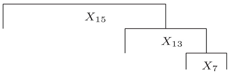
Final Tree Identified by Most Simulation Runs Using Collapsed Binary Responses.

Using this experiment, we re-evaluated the idea of treating the ordinal responses as continuous ones. Table 3 summarizes all of the final tree structures. Like the dichotomization approach, this approach does not perform as well as the use of h(t) in (6).

Table 3.

Distinct Final Trees and Their Frequencies In 50 Simulation Runs by Treating Ordinal Responses as Continuous Measures

Frequency	Tree Structure
27
12
10
1

4. APPLICATION

We now apply our method to the BROCS data set analyzed by Zhang (1998). BROCS contains a set of highly correlated symptoms of discomfort reported by occupants of buildings. It is a common occurrence in office buildings, hospitals, etc. all over the world. There are several common symptoms of BROCS such as irritation of the eyes, nose, and throat, headache, and nausea. Continuing efforts have been dedicated to understand the nature and find the cause of BROCS. See Zhang (1998) for the related references. Our data set is a subset of the data from a 1989 survey of 6,800 employees of the Library of Congress (LOC) and the headquarters of the Environmental Protection Agency (EPA) in the United States. In Zhang (1998), BROCS is represented by six binary outcome variables in Table 1, and 22 predictors described in Table 2 are considered as risk factors of BROCS. While we use the same covariates, because the six outcome variables were originally defined in ordinal scales, we reanalyze the data set using the six three-level ordinal responses (0: rarely; 1: sometimes; 2: often).

Table 1.

Ordinal Response Variables

Response	Cluster	Symptoms
y1	CNS	Difficulty remembering/concentrating, dizziness, lightheadedness
y2	Upper airway	Runny/stuffy nose, sneezing, cough, sore throat
y3	Pain	Aching muscles/joints, pain in back/shoulders/neck, pain in hands/wrists
y4	Flu-like	Nausea, chills, fever
y5	Eyes	Dry, itching, or tearing eyes; sore/strained eyes; blurry vision
y6	Lower airway	Wheezing in chest, shortness of breath, chest tightness

Table 2.

Description of Explanatory Variables

Name	Questions	Answer
x1	What is the type of your working space?	enclosed office with door, cubicle without door, stacks, etc.
x2	How is your working space shared	single, occupant, shared, etc.
x3	Do you have a metal desk?	yes or no
x4	Do you have new equipment at your work area?	yes or no
x5	Are you allergic to pollen?	yes or no
x6	Are you allergic to dust?	yes or no
x7	Are you allergic to mold?	yes or no
x8	How old are you?	16–79 years old
x9	Gender	male or female
x10	Is there too much air movement at your work area?	never, rarely, sometimes, often, always
x11	Is there too little air movement at your work area?	same as x10
x12	Is your work area too dry?	same as x10
x13	Is the air too stuffy at your work area?	same as x10
x14	Is your work area too noisy?	same as x10
x15	Is your work area too dusty?	same as x10
x16	Do you experience glare at your workstation?	no, sometimes, often, always
x17	How comfortable is your chair?	reasonably, somewhat, very uncomfortable, no one specific chair
x18	Is your chair easily adjustable?	yes, no, not adjustable
x19	Do you have influence over arranging the furniture?	very little, little, moderate, much, very much
x20	Do you have children at home?	yes or no
x21	Do you have major childcare duties?	yes or no
x22	what type of job do you have?	managerial, professional, technical, etc.

Based on (5), an initial tree T₀ of 103 nodes was grown. The pruning step produced a sequence of 52 nested optimal subtrees. The cost-complexity plot for these nested subtrees is displayed in Figure 3. Ten replications of 5-fold cross-validation were used to obtain the estimates of the subtree costs and their standard errors. As can be seen in Figure 3, the 1-standard error rule leads to the final subtree with 15 terminal nodes, which is displayed in Figure 4. This figure also summarizes the information for the 15 terminal nodes.

Figure 3.

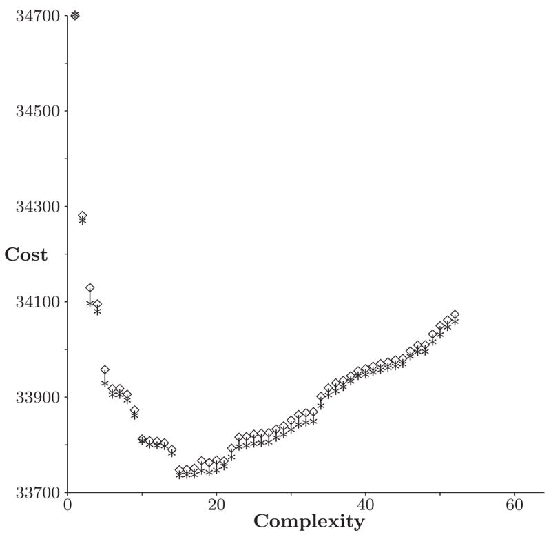
Cost-Complexity for Sequence of Nested Subtrees. ***, Cross-Validation Estimates of Cost; ⋄ ⋄ ⋄, One Standard Error Above the Cross-Validation Estimated Cost.

Figure 4.

Tree Structure for the Risk Factors of BROCS. Each Terminal Node is Represented by a 3 × 6 Table in which Rows Correspond to Levels of Response 0, 1, 2 from Bottom Up and Columns to the 6 Multivariate Responses. From Left to Right, They Are CNS, UA, Pain, Flu-like, Eyes, and LA. Each Cell Is Colored by Its Corresponding Frequency with the Color Scale Displayed on Top of Node 27.

Figure 4 reveals more information than that presented by Zhang (1998). First, it includes all risk factors related to air quality measures that were identified by Zhang (1998). Furthermore, it suggests that subjects in terminal nodes 16 and 17 reported the fewest numbers of complaints for all six types of symptoms. People in those groups experienced better air quality in their working environment. For example, the air was never too dusty, rarely too dry, and might be occasionally too stuffy. Comparison of nodes 16 to 17, and 22 to 23 reveals the gender difference in that females complained more frequently of discomfort than males, especially for pain.

Even though subjects in terminal nodes 24 and 25 were allergic to mold, comparison of these nodes suggests that a too dusty air quality in the work space resulted in more frequent discomfort in the upper airway and pain.

It is interesting to note that Zhang (1998) did not note a clear increase of discomfort of eye symptoms as a result of experiencing a glare. Examining terminal nodes 26 and 27 suggests a notable increase of eye symptoms at level 2, although this is less notable at level 1. An increase of comfort in some of the other symptoms is more apparent.

Figure 4 reveals that the variation in the level 1 responses among all terminal nodes is relatively modest for every symptom. In other words, the 22 covariates are not so predictive at this discomfort level. The variation in the level 2 responses is evident, although as noted by Zhang (1998) the eyes-related complaints are quite rare in general. In contrast to Zhang (1998) in which levels 1 and 2 were merged, our analysis suggests that it would have been more reasonable to merge levels 0 and 1. In other words, if collapsing some levels are desirable, our proposed method can provide useful information as to how the collapsing should be executed.

5. DISCUSSION

We proposed a tree-based method to analyze multivariate ordinal responses. Our method is semiparametric and takes advantage of the adaptive and intuitive tree structures as well as the simplicity of parametric assumptions. While this general idea appears straightforward, developing a computationally feasible and practically interpretable approach remains a challenge.

It is very common for multivariate ordinal responses to have missing data. For example, in longitudinal analysis, missing values occur when the subject of interest is unavailable for the measurements. In our analysis, we assumed that the number of observations are equal for each subject. Since missing data in the response variables result in a varying number of observations for each subject, it remains important to investigate multiple imputation schemes in the context of tree based modeling.

While we have examined multivariate responses with the same number of ordinal scales, our model and method are readily applicable to a mix of ordinal and nominal responses, including the binary case. The challenge is to define a tractable and justifiable joint distribution.

Unlike parametric methods that are best suited for data with simple relations in the data, tree-based approach is more advantageous for data that include a large number of covariates and response variables, such as the BROCS data set. We have demonstrated through simulation studies that our method can perform exploratory data analysis, choose the important covariates from a long list of potentially influential covariates, and unravel the appropriate data structures. Applying our method to the BROCS data set led to useful insights into the understanding of the BROCS.

Dealing with multivariate responses, binary or ordinal, is a challenging and complicated task. Compared to the modeling of multiple binary responses, the task is even more complex for multiple ordinal responses. In an effort to reduce the computational burden, we proposed and evaluated a time-saving algorithm for optimization. A continuing effort to improve the computational efficiency remains worthwhile.

Through the analysis of a specific data set, we see that there are some clear advantages of analyzing ordinal responses. By beginning with the ordinal responses, we may also find helpful information to collapse the responses if we want to simplify the data and analysis.

Many other topics are worthwhile for future investigations. In this work, we focused on establishing an adaptive framework. In addition to the important issues mentioned above, with a large number of predictors, there may be alternative and competitive tree structures. To learn and utilize as much information as possible from such a data set, it is useful to consider forests such as bagging (Breiman 1996) and deterministic procedures (Zhang et al. 2003). Finally, Bayesian approach is also worth pursuing.

APPENDIX: COMPUTATIONAL ISSUES

It follows from the node specific likelihood function (2) that

$$\left(\begin{array}{l}\frac{\partial }{\partial {\psi }_i}\hfill \\ \frac{\partial }{\partial {\theta }_i}\hfill \end{array}\right)log{f}_i=\left(\begin{array}{l}{y}_i-E(Y_i)\hfill \\ w_i-E(W_i)\hfill \end{array}\right).$$

Using the link matrices defined in (4) and based on model (5), we have

$$\begin{array}{ll}\left(\begin{array}{l}\frac{\partial }{\partial \psi }\hfill \\ \frac{\partial }{\partial \theta }\hfill \end{array}\right)log{f}_i& =\left(\begin{array}{ll}\frac{\partial {\psi }_i}{\partial \psi }\hfill & 0\hfill \\ 0\hfill & \frac{\partial {\theta }_i}{\partial \theta }\hfill \end{array}\right)\left(\begin{array}{l}\frac{\partial }{\partial {\psi }_i}\hfill \\ \frac{\partial }{\partial {\theta }_i}\hfill \end{array}\right)log{f}_i\\ & =\left(\begin{array}{ll}B\hfill & 0\hfill \\ 0\hfill & C^T\hfill \end{array}\right)\left(\begin{array}{l}{y}_i-E(Y_i)\hfill \\ w_i-E(W_i)\hfill \end{array}\right),\end{array}$$

where B = I_n×(K−1) and C is defined in (4).

The likelihood function from the N units of observations is

$$f(z,\psi ,\theta )=\prod _{i=1}^N{f}_i(z_i,\psi ,\theta ),$$

and the log-likelihood is

$$l(z,\psi ,\theta )=\sum _{i=1}^N{l}_i(z_i,\psi ,\theta )=\sum _{i=1}^{N}log{f}_i(z_i,\psi ,\theta ).$$

Thus, the score equations are

$$\left(\begin{array}{l}\frac{\partial }{\partial \psi }\hfill \\ \frac{\partial }{\partial \theta }\hfill \end{array}\right)logf=\sum _{i=1}^N\left(\begin{array}{ll}B\hfill & 0\hfill \\ 0\hfill & C^T\hfill \end{array}\right)\left(\begin{array}{l}{y}_i-E(Y_i)\hfill \\ w_i-E(W_i)\hfill \end{array}\right).$$

To find ψ̂ and θ̂ that maximize the log-likelihood l(z, ψ, θ), we tested Newton’s method, Quasi-Newton method and our simplified iteration procedure. The updating formula for Newton’s method is listed below

$$\begin{array}{ll}{\left(\begin{array}{l}\psi \hfill \\ \theta \hfill \end{array}\right)}^{(J+1)}=& {\left(\begin{array}{l}\psi \hfill \\ \theta \hfill \end{array}\right)}^{(J)}\\ & +{(V^{(J)})}^{-1}\sum _{i=1}^N\left(\begin{array}{ll}B\hfill & 0\hfill \\ 0\hfill & C^T\hfill \end{array}\right)\left(\begin{array}{l}{y}_i-E(Y_i)\hfill \\ w_i-E(W_i)\hfill \end{array}\right),\end{array}$$ (12)

where V^(J) is the covariance matrix of (Y, W) at the J-th step. As noted in Zhang (1998), however, the computation for updating the estimators, especially the computation of (V^(J))⁻¹ can be very time consuming. Also as the number of repeated response n increases, the method rarely converges. For example, when n = 6, the Newton’s method rarely converged.

The BFGS method is one of the Quasi-Newton methods that avoids computing the inverse Hessian matrix. It calculates the score function and approximates the inverse Hessian matrix at step k. Let ν = {ψ, θ}. We first choose a initial guess ν₀ and set B₀ = I, the identity matrix. At the k + 1-th step of BFGS method, we proceed as follows:

1. Compute the score function s_k+1. If s_k+1=0, stop. Otherwise, let d_k+1 = B_ks_k+1 (B_k is the approximation of the inverse Hessian matrix).

2. Perform a linear search to find the optimal step length α_k+1 and set ν_k+1 = ν_k + α_k+1s_k+1.

3. Update B_k+1, the approximation of inverse Hessian matrix. Let ν_k = s_k+1 − s_k and w_k = ν_k+1 − ν_k, then

$$B_{k+1}=B_k+\left(1+\frac{v_k^{\prime }{B}_k{v}_k}{v_k^{\prime }{w}_k}\right)\frac{w_k{w}_k^{\prime }}{v_k^{\prime }{w}_k}-\frac{B_k{v}_k{w}_k^{\prime }+w_k{v}_k^{\prime }{B}_k}{v_k^{\prime }{w}_k}.$$

The computation for BFGS method is also very extensive. It includes several vector and matrix operations during each updating step.

We adopt and verify a simplified iteration procedure to reduce the computational burden. Specifically, we use the sample variance-covariance matrix V₀ of

$$\left(\begin{array}{ll}B\hfill & 0\hfill \\ 0\hfill & C^T\hfill \end{array}\right)\left(\begin{array}{l}{y}_i\hfill \\ w_i\hfill \end{array}\right)$$

and update the estimators of the parameters ψ and θ as follows:

$$\begin{array}{ll}{\left(\begin{array}{l}\psi \hfill \\ \theta \hfill \end{array}\right)}^{(J+1)}=& {\left(\begin{array}{l}\psi \hfill \\ \theta \hfill \end{array}\right)}^{(J)}\\ & +V_0^{-1}\sum _{i=1}^N\left(\begin{array}{ll}B\hfill & 0\hfill \\ 0\hfill & C^T\hfill \end{array}\right)\left(\begin{array}{l}{y}_i-E(Y_i)\hfill \\ w_i-E(W_i)\hfill \end{array}\right).\end{array}$$ (13)

We report our simulation study to validate our simplified maximization procedure. Using model (5), we generate N units of observations, ${\{Y_i={(Y_{i1},\dots ,Y_{in})}^T\}}_{i=1}^N$, where N is chosen from 100 and 200. We consider the following four settings for n: (a) n=3; (b) n=4; (c) n=5; and (d) n=6. The level K for the ordinal response is set to 3. The parameters to be estimated are ψ₁₁, ψ₁₂,…, ψ _(n−1),1, ψ _(n−1),2, θ₁₁, θ₁₂, θ₂₁, θ₂₂.

Tables 4, 5, 6, and 7 report parameter estimates and their standard errors for the four settings of n, using our simplified method and the Quasi-Newton method. The results show that the simplified estimation procedure performs nearly identically to the Quasi-Newton method in all settings. It is also interesting to note that when n = 6, the Quasi-Newton method significantly underestimates the ψ while our proposed simplified procedure has sufficient accuracy. As expected, an increased sample size improves the accuracy of the parameter estimates. Table 8 displays the dramatic savings in terms of computational time. In summary, Tables 4, 5, 6, 7, and 8 demonstrate that the simplified algorithm reduces computation time by 20 to 160 folds while maintaining the same or better level of accuracy as the Quasi-Newton method. This saving of computational time is significant in the present context because the selection of splits and the determination of the tree require numerous rounds of maximizing the likelihoods.

Table 4.

Comparison of Parameter Estimates Between the Simplied Method and the Quasi-Newton Algorithm when the Response is 3-Dimensional (1000 Replications)

	True Value	N=300				N=400
		Simplified Method		Quasi-Newton		Simplified Method		Quasi-Newton
		Estimate	S.E.	Estimate	S.E.	Estimate	S.E.	Estimate	S.E.
ψ11	−.75	−0.75	0.20	−0.75	0.20	−0.75	0.17	−0.75	0.17
ψ12	−1.	−1.02	0.29	−1.02	0.29	−1.02	0.25	−1.02	0.25
ψ21	−.75	−0.75	0.19	−0.75	0.19	−0.75	0.17	−0.75	0.17
ψ22	−1.	−1.00	0.24	−1.00	0.24	−1.01	0.20	−1.01	0.20
ψ31	−.75	−0.75	0.19	−0.75	0.19	−0.74	0.16	−0.74	0.17
ψ32	−1.	−1.00	0.29	−1.00	0.29	−1.01	0.25	−1.00	0.25
θ11	0.25	0.24	0.16	0.24	0.16	0.24	0.16	0.24	0.15
θ12	0.25	0.25	0.22	0.25	0.22	0.25	0.20	0.25	0.20
θ21	0.25	0.26	0.23	0.26	0.23	0.26	0.20	0.26	0.20
θ22	0.25	0.24	0.25	0.24	0.25	0.24	0.22	0.24	0.22

Table 5.

Comparison of Parameter Estimates Between the Simplied Method and the Quasi-Newton Algorithm when the Response is 4-Dimensional (1000 Replications)

	True Value	N=300				N=400
		Simplified Method		Quasi-Newton		Simplified Method		Quasi-Newton
		Estimate	S.E.	Estimate	S.E.	Estimate	S.E.	Estimate	S.E.
ψ11	−.75	−0.74	0.22	−0.74	0.22	−0.75	0.20	−0.75	0.20
ψ12	−1.	−1.01	0.30	−1.01	0.30	−1.00	0.27	−1.00	0.26
ψ21	−.75	−0.75	0.21	−0.75	0.21	−0.75	0.18	−0.75	0.18
ψ22	−1.	−1.01	0.24	−1.01	0.24	−1.01	0.21	−1.00	0.21
ψ31	−.75	−0.74	0.20	−0.74	0.20	−0.74	0.18	−0.74	0.18
ψ32	−1.	−1.03	0.25	−1.03	0.25	−1.02	0.22	−1.01	0.22
ψ41	−.75	−0.74	0.21	−0.74	0.21	−0.74	0.19	−0.74	0.19
ψ42	−1.	−1.01	0.29	−1.01	0.29	−1.00	0.25	−1.00	0.25
θ11	0.25	0.24	0.12	0.24	0.12	0.24	0.10	0.24	0.10
θ12	0.25	0.26	0.14	0.26	0.14	0.25	0.12	0.25	0.12
θ21	0.25	0.25	0.15	0.25	0.14	0.25	0.13	0.25	0.13
θ22	0.25	0.25	0.14	0.25	0.14	0.25	0.12	0.25	0.12

Table 6.

Comparison of Parameter Estimates Between the Simplied Method and the Quasi-Newton Algorithm when the Response is 5-Dimensional (1000 Replications)

	True Value	N=300				N=400
		Simplified Method		Quasi-Newton		Simplified Method		Quasi-Newton
		Estimate	S.E.	Estimate	S.E.	Estimate	S.E.	Estimate	S.E.
ψ11	−.75	−0.75	0.28	−0.75	0.25	−0.75	0.25	−0.75	0.22
ψ12	−1.	−1.00	0.33	−0.99	0.30	−1.01	0.28	−1.00	0.25
ψ21	−.75	−0.74	0.27	−0.75	0.25	−0.74	0.24	−0.74	0.21
ψ22	−1.	−1.01	0.26	−1.00	0.23	−1.01	0.21	−1.00	0.20
ψ31	−.75	−0.74	0.27	−0.74	0.25	−0.74	0.23	−0.74	0.21
ψ32	−1.	−1.02	0.25	−1.00	0.23	−1.02	0.21	−1.00	0.19
ψ41	−.75	−0.75	0.26	−0.75	0.24	−0.75	0.23	−0.75	0.20
ψ42	−1.	−1.01	0.27	−0.99	0.24	−1.01	0.24	−0.99	0.21
ψ51	−.75	−0.74	0.27	−0.74	0.25	−0.74	0.24	−0.74	0.22
ψ52	−1.	−1.02	0.34	−1.00	0.31	−1.01	0.29	−1.00	0.26
θ11	0.25	0.24	0.11	0.25	0.09	0.24	0.10	0.25	0.08
θ12	0.25	0.26	0.11	0.25	0.10	0.26	0.10	0.25	0.09
θ21	0.25	0.26	0.12	0.25	0.10	0.26	0.10	0.25	0.09
θ22	0.25	0.24	0.09	0.25	0.09	0.24	0.08	0.25	0.07

Table 7.

Comparison of Parameter Estimates Between the Simplied Method and the Quasi-Newton Algorithm when the Response is 6-Dimensional (1000 Replications)

	True Value	N=300				N=400
		Simplified Method		Quasi-Newton		Simplified Method		Quasi-Newton
		Estimate	S.E.	Estimate	S.E.	Estimate	S.E.	Estimate	S.E.
ψ11	−.75	−0.72	0.50	−0.62	0.34	−0.72	0.43	−0.60	0.30
ψ12	−1.	−0.99	0.47	−0.99	0.35	−1.00	0.40	0.98	0.30
ψ21	−.75	−0.70	0.47	−0.60	0.31	−0.70	0.41	−0.59	0.27
ψ22	−1.	−1.00	0.38	−0.99	0.28	−1.00	0.33	0.99	0.24
ψ31	−.75	−0.71	0.47	−0.61	0.31	−0.71	0.40	−0.60	0.26
ψ32	−1.	−1.00	0.33	−0.98	0.24	−1.00	0.28	−0.98	0.21
ψ41	−.75	−0.71	0.46	−0.61	0.30	−0.71	0.39	−0.60	0.26
ψ42	−1.	−1.01	0.33	−0.99	0.24	−1.01	0.28	−0.99	0.21
ψ51	−.75	−0.69	0.47	−0.59	0.32	−0.70	0.41	−0.60	0.27
ψ52	−1.	−1.01	0.38	−0.99	0.28	−1.00	0.32	−0.98	0.24
ψ61	−.75	−0.70	0.49	−0.60	0.33	−0.70	0.42	−0.59	0.29
ψ62	−1.	−1.02	0.46	−1.01	0.36	−1.02	0.39	−1.00	0.30
θ11	0.25	0.24	0.14	0.22	0.07	0.24	0.12	0.21	0.06
θ12	0.25	0.26	0.12	0.26	0.09	0.26	0.10	0.25	0.08
θ21	0.25	0.25	0.12	0.25	0.09	0.25	0.10	0.25	0.08
θ22	0.25	0.25	0.07	0.25	0.07	0.25	0.06	0.25	0.06

Table 8.

Comparison of Running Time Between the Simplified Method and the Quasi-Newton Method (in Seconds)

	N=300				N=400
ni	3	4	5	6	3	4	5	6
Simplified Method	6	13	30	759	7	14	29	293
Quasi-Newton	387	1368	4100	16680	480	1699	4705	17978

References

- Agresti A. Modelling ordered categorical data: recent advances and future challenges. Statistics in Medicine. 1999;18:2191–2207. doi: 10.1002/(sici)1097-0258(19990915/30)18:17/18<2191::aid-sim249>3.0.co;2-m. [DOI] [PubMed] [Google Scholar]
- Breiman L. Bagging predictors. Machine Learning. 1996;24:123–140. [Google Scholar]
- Breiman L, Friedman JH, Olshen RA, Stone CJ. Classification and Regression Tress. Pacific Grove, CA: Wadsworth; 1984. [Google Scholar]
- Esposito F, Malerba D, Semeraro G. A comparative analysis of methods for pruning decision trees. IEEE Transactions on Pattern Analysis and Machine Intelligence. 1997;19(5):476–491. [Google Scholar]
- Hedeker D, Gibbons RD. A random-effects ordinal regression model for multilevel analysis. Biometrics. 1994;50:933–944. [PubMed] [Google Scholar]
- Kauermann G. Modeling longitudinal data with ordinal response by varying coefficients. Biometrics. 2000;56:692–698. doi: 10.1111/j.0006-341x.2000.00692.x. [DOI] [PubMed] [Google Scholar]
- Li X, Sweigart J, Teng J, Donohue J, Thombs L. A dynamic programming based pruning method for decision trees. Journal on Computing. 2001;13:332–345. [Google Scholar]
- Mingers J. Expert systems – rule induction with statistical data. J Operational Research Society. 1987;28:39–47. [Google Scholar]
- Niblett T, Bratko I. Proc Expert Systems. Vol. 86. Cambridge: Cambridge University Press; 1986. Learning Decision Rules in Noisy Domains. [Google Scholar]
- Quinlan JR. Simplifying decision tree. Machine Learning. 1987;1:221–234. [Google Scholar]
- Quinlan JR. C4.5: Programs for Machine Learning. Morgan Kaufmann; San Mateo, CA: 1993. [Google Scholar]
- Segal MR. Tree-structured methods for longitudinal data. Journal of the American Statistical Association. 1992;87:407–418. [Google Scholar]
- Ten Have TR. A mixed effects model for multivariate ordinal response data including correlated discrete failure times with ordinal responses. Biometrics. 1996;52:473–491. MR139500. [PubMed] [Google Scholar]
- Zhang HP. Multivariate adaptive splines for analysis of longitudinal data. Journal of Computational and Graphical Statistics. 1997;6:74–91. MR145199. [Google Scholar]
- Zhang HP. Classification trees for multiple binary responses. Journal of the American Statistical Association. 1998;93(441):180–193. [Google Scholar]
- Zhang HP, Feng R, Zhu HT. A latent variable model of segregation analysis for ordinal traits. Journal of the American Statistical Association. 2003;98(464):1023–1034. MR2041490. [Google Scholar]
- Zhang HP, Singer B. Recursive Partitioning in the Health Science. New York: Springer; 1999. MR1683316. [Google Scholar]
- Zhang HP, Wang X, Ye Y. Detection of genes for ordinal traits in nuclear families and a unified approach for association studies. Genetics. 2006;172:693–699. doi: 10.1534/genetics.105.049122. [DOI] [PMC free article] [PubMed] [Google Scholar]