

Abstract
The LASSO-Patternsearch algorithm is proposed to efficiently identify patterns of multiple dichotomous risk factors for outcomes of interest in demographic and genomic studies. The patterns considered are those that arise naturally from the log linear expansion of the multivariate Bernoulli density. The method is designed for the case where there is a possibly very large number of candidate patterns but it is believed that only a relatively small number are important. A LASSO is used to greatly reduce the number of candidate patterns, using a novel computational algorithm that can handle an extremely large number of unknowns simultaneously. The patterns surviving the LASSO are further pruned in the framework of (parametric) generalized linear models. A novel tuning procedure based on the GACV for Bernoulli outcomes, modified to act as a model selector, is used at both steps. We applied the method to myopia data from the population-based Beaver Dam Eye Study, exposing physiologically interesting interacting risk factors. We then applied the the method to data from a generative model of Rheumatoid Arthritis based on Problem 3 from the Genetic Analysis Workshop 15, successfully demonstrating its potential to efficiently recover higher order patterns from attribute vectors of length typical of genomic studies.
1. INTRODUCTION
We consider the problem which occurs in demographic and genomic studies when there are a large number of risk factors that potentially interact in complicated ways to induce elevated risk. The goal is to search for important patterns of multiple risk factors among a very large number of candidate patterns, with results that are easily interpretable. In this work the LASSO-Patternsearch algorithm (LPS) is proposed for this task. All variables are binary, or have been dichotomized before the analysis, at the risk of some loss of information; this allows the study of much higher order interactions than would be possible with risk factors with more than several possible values, or with continuous risk factors. Thus LPS may, if desired, be used as a preprocessor to select clusters of variables that are later analyzed in their pre-dichotomized form, see [39]. Along with demographic studies, a particularly promising application of LPS is to the analysis of patterns or clusters of SNPs (Single Nucleotide Polymorphisms) or other genetic variables that are associated with a particular phenotype, when the attribute vectors are very large and there exists a very large number of candidate patterns. LPS is designed specifically for the situation where the number of candidate patterns may be very large, but the solution, which may contain high order patterns, is believed to be sparse. LPS is based on the log linear parametrization of the multivariate Bernoulli distribution [35] to generate all possible patterns, if feasible, or at least a large subset of all possible patterns up to some maximum order. LPS begins with a LASSO algorithm (penalized Bernoulli likelihood with an l1 penalty), used with a new tuning score, BGACV. BGACV is a modified version of the GACV score [37] to target variable selection, as opposed to Kullback-Liebler distance, which is the GACV target. A novel numerical algorithm is developed specifically for this step, which can handle an extremely large number of basis functions (patterns) simultaneously. This is in particular contrast to most of the literature in the area, which uses greedy or sequential algorithms. The patterns surviving this process are then entered into a parametric linear logistic regression to obtain the final model, where further sparsity may be enforced via a backward elimination process using the BGACV score as a stopping criterion. Properties of LPS will be examined via simulation, and in demographic data by scrambling responses to establish false pattern generation rates.
There are many approaches that can model data with binary covariates and binary responses, see, for example CART [1], LOTUS [2], Logic regression [27] and Stepwise Penalized Logistic Regression (SPLR) [26]. Logic regression is an adaptive regression methodology that constructs predictors as Boolean combinations of binary covariates. It uses simulated annealing to search through the high dimensional covariate space and uses five-fold cross validation and randomization based hypothesis testing to choose the best model size. SPLR is a variant of logistic regression with l2 penalty to fit interaction models. It uses a forward stepwise procedure to search through the high dimensional covariate space. The model size is chosen by an AIC- or BIC-like score and the smoothing parameter is chosen by 5-fold cross validation. For Gaussian data the LASSO was proposed in [32] as a variant of linear least squares ridge regression with many predictor variables. As proposed there, the LASSO minimized the residual sum of squares subject to a constraint that the sum of absolute values of the coefficients of the basis functions be less than some constant, say t. This is equivalent to minimizing the residual sum of squares plus a penalty which is some multiple λ (depending on t) of the sum of absolute values (l1 penalty). It was demonstrated there that this approach tended to set many of the coefficients to zero, resulting in a sparse model, a property not generally obtaining with quadratic penalties. A similar idea was exploited in [3] to select a good subset of an over-complete set of nonorthogonal wavelet basis functions. The asymptotic behavior of LASSO type estimators was studied in [16], and [25] discussed computational procedures in the Gaussian context. More recently [5] discussed variants of the LASSO and methods for computing the LASSO for a continuous range of values of λ in the Gaussian case. Variable selection properties of the LASSO were examined in [20] in some special cases, and many applications can be found on the web. In the context of nonparametric ANOVA decompositions [39] used an overcomplete set of basis functions obtained from a Smoothing Spline ANOVA model, and used ℓ1 penalties on the coefficients of main effects and low order interaction terms, in the spirit of [3]. The present paper uses some ideas from [39], although the basis function set here is quite different. Other work has implemented ℓ1 penalties along with quadratic (reproducing kernel square norm) penalties to take advantage of the properties of both kinds of penalties, see for example [12, 19, 38, 40].
The rest of the article is organized as follows. In Section 2 we describe the first (LASSO) step of the LPS including choosing the smoothing parameter by the B-type Generalized Approximate Cross Validation (BGACV), “B” standing for the prior belief that the solution is sparse, analogous to BIC. An efficient algorithm for the LASSO step is presented here. Section 3 describes the second step of the LASSO-Patternsearch algorithm, utilizing a parametric logistic regression, again tuned by BGACV. Section 4 presents three simulation examples, designed to demonstrate the properties of LPS as well as comparing LPS to Logic regression and SPLR. Favorable properties of LPS are exhibited in models with high order patterns and correlated attributes. Section 5 applies the method to myopic changes in refraction in an older cohort from the Beaver Dam Eye Study [15], where some interesting risk patterns including one involving smoking and vitamins are found. Section 6 applies the method to data from a generative model of Rheumatoid Arthritis Single Nucleotide Polymorphisms adapted from the Genetics Analysis Workshop 15 [6], which examines the ability of the algorithm to recover third order patterns from extremely large attribute vectors. Section 7 notes some generalizations, and, finally, Section 8 gives a summary and conclusions. Appendix A derives the BGACV score; Appendix B gives details of the specially designed code for the LASSO which is capable of handling a very large number of patterns simultaneously; Appendix C shows the detailed results of Simulation Example 3. When all of the variables are coded as 1 in the risky direction, the model will be sparsest among equivalent models. Appendix D gives a lemma describing what happens when some of the variables are coded with the opposite direction as 1.
2. THE LASSO-PATTERNSEARCH ALGORITHM
2.1 The LASSO-Patternsearch algorithm –Step 1
Considering n subjects, for which p variables are observed, we first reduce continuous variables to “high” or “low” in order to be able to examine very many variables and their interactions simultaneously. We will assume that for all or most of the the p variables, we know in which direction they are likely to affect the outcome or outcomes of interest, if at all. For some variables, for example smoking, it is clear for most endpoints in which direction the smoking variable is likely to be “bad” if it has any effect, and this is true of many but not all variables. For some continuous variables, for example systolic blood pressure, higher is generally “worse”, but extremely low can also be “bad”. For continuous variables, we need to initially assume the location of a cut point on one side of which the variable is believed to be “risky” (“high”) and the other side “not risky” (“low”). For systolic blood pressure that might, for example, be 140 mmHg. For an economic variable, that might be something related to the current standard for poverty level. If the “risky” direction is known for most variables the results will be readily interpretable. Each subject thus has an attribute vector of p zeroes and ones, describing whether each of their p attributes is on one side or the other of the cutoff point. The LASSO-Patternsearch approach described below is able to deal with high order interactions and very large p. The data is {yi, x(i), i = 1, …, n}, where yi ∈ {0, 1} codes the response, x(i) = (x1(i), x2(i), …, xp(i)) is the attribute vector for the ith subject, xj (i) ∈{0, 1}. Define the basis functions , that is, Bj1j2..jr (x) = 1 if xj1, …, xjr are all 1’s and 0 otherwise. We will call Bj1j2.. jr (x) an rth order pattern. Let q be the highest order we consider. Then there will be patterns. If q = p, we have a complete set of NB = 2p such patterns (including the constant function μ), spanning all possible patterns. If q = 1 only first order patterns (henceforth called “main effects”) are considered, if q = 2 main effects and second order patterns are considered, and so forth. Letting p(x) = Prob[y = 1|x] and the logit (log odds ratio) be f (x) = log[p(x)/(1 − p(x))], we estimate f by minimizing
| (1) |
where is times the negative log likelihood:
| (2) |
with
| (3) |
where we are relabeling the NB −1 (non-constant) patterns from 1 to NB −1, and
| (4) |
If all possible patterns are included in (3) then f there is the most general form of the log odds ratio for y given x obtainable from the log linear parametrization of the multivariate Bernoulli distribution given in [35]. In Step 1 of the LASSO-Patternsearch we minimize (1) using the BGACV score to choose λ. The next section describes the BGACV score and the kinds of results it can be expected to produce.
2.2 B-type Generalized Approximate Cross Validation (BGACV)
The tuning parameter λ in (1) balances the trade-off between data fitting and the sparsity of the model. The bigger λ is, the sparser the model. The choice of λ is generally a crucial part of penalized likelihood methods and machine learning techniques like the Support Vector Machine. For smoothing spline models with Gaussian data, [34] proposed ordinary leave-out-one cross validation (OCV). Generalized Cross Validation (GCV), derived from OCV, was proposed in [4, 11], and theoretical properties were obtained in [21] and elsewhere. For smoothing spline models with Bernoulli data and quadratic penalty functionals, [37] derived the Generalized Approximate Cross Validation (GACV) from an OCV estimate following the method used to obtain GCV. In [39] GACV was extended to the case of Bernoulli data with continuous covariates and l1 penalties.
The derivation of the GACV begins with a leaving-out-one likelihood to minimize an estimate of the comparative Kullback-Leibler distance (CKL) between the true and estimated model distributions. The ordinary leave-out-one cross validation score for CKL is
| (5) |
where fλ is the minimizer of the objective function (1), and is the minimizer of (1) with the ith data point left out. Through a series of approximations and an averaging step as described in Appendix A, we obtain the GACV score appropriate to the present context. It is a simple to compute special case of the GACV score in [39]:
| (6) |
here H = B*(B*′W B*)−1B*′, where W is the n × n diagonal matrix with iith element the estimated variance at x(i) (piλ(1 −piλ)) and B* is the n × NB0 design matrix for the NB0 non-zero cℓ in the model. The quantity plays the role of degrees of freedom here. As is clear from the preceding discussion, the GACV is a criterion whose target is the minimization of the (comparative) Kullback-Liebler distance from the estimate to the unknown “true” model. By analogy with the Gaussian case (where the predictive mean squared error and comparative Kullback-Liebler distance coincide), it is known that optimizing for predictive mean square error and optimizing for model selection when the true model is sparse are not in general the same thing. This is discussed in various places, for example, see [10] which discusses the relation between AIC and BIC, AIC being a predictive criterion and BIC, which generally results in a sparser model, being a model selection criterion, with desirable properties when the “true” model is of fixed (low) dimension as the sample size gets large. See also [13, 20] and particularly our remarks at the end of Appendix A. In the AIC to BIC transformation, if γ is the degrees of freedom for the model, then BIC replaces γ with . By analogy we obtain a model selection criterion, BGACV, from GACV as follows. Letting γ be the quantity playing the role of degrees of freedom for signal in the Bernoulli-l1 penalty case,
| (7) |
γ is replaced by to obtain
| (8) |
We illustrate the difference of empirical performances between GACV and BGACV on a “true” model with a small number of strong patterns. Let , and be independently distributed from a bivariate normal distribution with mean 0, variance 1 and covariance 0.7. Xi = 1 if and 0 otherwise, i = 1, 2, …, 6. X7 is independent of the others and takes two values {1, 0}, each with a probability of 0.5. X = (X1, …, X7). The sample size n = 800. Three patterns that consist of six variables are important, and X7 is noise. The true logit is
| (9) |
This problem is very small so we chose the maximum order q = p = 7, so 127 patterns plus a constant term are entered in the trial model. We ran the simulation 100 times and the result is shown in Table 1. Both GACV and BGACV select the three important patterns perfectly, but GACV selects more noise patterns than BGACV. Note that a total of 27−4 noise patterns have been considered in each run. The maximum possible number in the last column is 100 ×(27 −4) = 12, 400. Neither GACV or BGACV is doing a bad job but we will discuss a method to further reduce the number of noise patterns in Section 3. Figure 1 shows the scores of these two criteria in the first data set. BGACV selects a bigger smoothing parameter than GACV does. These scores are not continuous at the the point where a parameter becomes zero so we see jumps in the plots.
Table 1.
The Results of Simulation Example 1. The Second Through Fourth Columns Are the Appearance Frequencies of the Three Important Patterns in the 100 Runs. The Last Column Is the Total Appearance Frequency of All Other Patterns. The Second and Third Row Compare GACV and BGACV Within the First Step of LPS. The Fourth Through Sixth Rows, which Compare the Full LPS with Logic Regression and SPLR Will Be Discussed in Section 4.1
| Method | B1 | B23 | B456 | other |
|---|---|---|---|---|
| GACV | 100 | 100 | 100 | 749 |
| BGACV | 100 | 100 | 100 | 568 |
|
| ||||
| LPS | 97 | 96 | 98 | 34 |
| Logic | 100 | 94 | 94 | 64 |
| SPLR | 100 | 90 | 55 | 426 |
Figure 1.
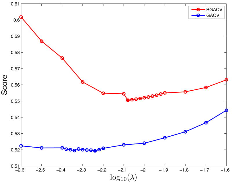
Comparison of BGACV and GACV in the First Data Set of Simulation Example 1. The Solid Dots Are The Minima. BGACV Selects a Bigger λ than GACV Does.
2.3 Computation
From a mathematical point of view, this optimization problem (1) is the same as the likelihood basis pursuit (LBP) algorithm in [39], but with different basis functions. The solution can easily be computed via a general constrained nonlinear minimization code such as MATLAB’s fmincon on a desktop, for a range of values of λ, provided n and NB are not too large. However, for extremely large data sets with more than a few attributes p (and therefore a large number NB of possible basis functions), the problem becomes much more difficult to solve computationally with general optimization software, and algorithms that exploit the structure of the problem are needed. We design an algorithm that uses gradient information for the likelihood term in (1) to find an estimate of the correct active set (that is, the set of components cℓ that are zero at the minimizer). When there are not too many nonzero parameters, the algorithm also attempts a Newton-like enhancement to the search direction, making use of the fact that first and second partial derivatives of the function in (1) with respect to the coefficients cℓ are easy to compute analytically once the function has been evaluated at these values of cℓ. It is not economical to compute the full Hessian (the matrix of second partial derivatives), so the algorithm computes only the second derivatives of the log likelihood function with respect to those coefficients cℓ that appear to be nonzero at the solution. For the problems that the LASSO-Patternsearch is designed to solve, just a small fraction of these NB coefficients are nonzero at the solution. This approach is similar to the two-metric gradient projection approach for bound-constrained minimization, but avoids duplication of variables and allows certain other economies in the implementation.
The algorithm is particularly well suited to solving the problem (1) for a number of different values of λ in succession; the solution for one value of λ provides an excellent starting point for the minimization with a nearby value of λ. Further details of this approach can be found in Appendix B.
3. THE LASSO-PATTERNSEARCH ALGORITHM – STEP 2
In Step 2 of LASSO-Patternsearch algorithm, the NB0 patterns surviving Step 1 are entered into a linear logistic regression model using glmfit in MATLAB and pattern selection is then carried out by the backward elimination method. We take out one of the NB0 patterns at a time, fit the model with the remaining patterns and compute the tuning score. The pattern that gives the best tuning score to the model after being taken out is removed from the model. This process continues until there are no patterns in the model. A final model is chosen from the pattern set with the best tuning score. Note that all-subset selection is not being done, since this will introduce an overly large number of degrees of freedom into the process.
If copious data is available, then a tuning set can be used to create the tuning score, but this is frequently not the case. Inspired by the tuning method in the LASSO step, we propose the BGACV score for the parametric logistic regression. The likelihood function is smooth with respect to the parameters so the robust assumption that appears in Appendix A is not needed. Other than that, the derivation of the BGACV score for parametric logistic regression follows that in Appendix A. Let s be the current subset of patterns under consideration and Bs be the design matrix. The BGACV score for logistic regression is the same as (8) with .
| (10) |
where fsi is the estimated log odds ratio for observation i and psi is the corresponding probability. The BGACV scores are computed for each model that is considered in the backward elimination procedure, and the model with the smallest BGACV score is taken as the final model.
The following is a summary of the LASSO-Patternsearch algorithm:
Solve (1) and choose λ by BGACV. Keep the patterns with nonzero coefficients.
Put the patterns with nonzero coefficients from Step 1 into a logistic regression model and select models by the backward elimination method with the selection criterion being BGACV.
For simulated data, the results can be compared with the simulated model. For observational data, a selective examination of the data will be used to validate the results. Other logistic regression codes, e.g. from R or SAS can be used instead of glmfit here.
4. SIMULATION STUDIES
In this section we study the empirical performance of the LPS through three simulated examples. The first example continues with simulated data in Section 2.2. There are three pairs of correlated variables and one independent variable. Three patterns are related to the response. The second example has only one high order pattern. The correlation within variables in the pattern is high and the correlation between variables in the pattern and other variables varies. The last example studies the performance of our method under various correlation settings. We compare LPS with two other methods, Logic regression [27] and Stepwise Penalized Logistic Regression (SPLR) [26]. We use the R package LogicReg to run Logic regression and the R package stepPlr to run SPLR. The number of trees and number of leaves in Logic regression are selected by 5-fold cross validation. The smoothing parameter in SPLR is also selected by 5-fold cross validation, and then the model size is selected by a BIC-like score based on an approximation to a degrees of freedom reproduced in the Comments section of Appendix A.
4.1 Simulation Example 1
In this example we have 7 variables and the sample size is 800. The true logit is f (x) = −2 + 1.5B1(x) + 1.5B23(x) + 2B456(x). The distribution of the covariates was described in Section 2.2. We simulated 100 data sets according to this model and ran all three methods on these data sets. The results are shown in the last three rows of Table 1.
Let’s compare LPS with the LASSO step (third row in Table 1) first. LPS misses all three patterns a few times. However, these numbers are still very close to 100 and more importantly, LPS significantly reduced the number of noise patterns, from over 500 to 34. Here we see why a second step is needed after the LASSO step. Now let’s look at LPS compared with the other two methods. Logic regression picks the first term perfectly but it doesn’t do as well as LPS on the remaining two patterns. It also selects more noise patterns than LPS. SPLR does worse, especially on the last pattern. It is not surprising because this example is designed to be difficult for SPLR, which is a sequential method. In order for B456 to be in the model, at least one main effect of X4, X5 and X6 should enter the model first, say X4. And then a second order pattern should also enter before B456. It could be B45 or B46. However, none of these lower order patterns are in the true model. This makes it very hard for SPLR to consider B456, and the fact that variables in the higher order pattern are correlated with variables in the lower order patterns makes it even harder. We also notice that SPLR selects many more noise patterns than LPS and Logic regression. Because of the way it allows high order patterns to enter the model, the smallest SPLR model has 6 terms, B1, one of B2 and B3, B23, one main effect and one second order pattern in B456, and B456. Conditioning on the appearance frequencies of the important patterns, SPLR has to select at least 90 + 2 × 55 = 200 noise patterns. The difference, 426 −200 = 226 is still much bigger than 34 selected by LPS.
4.2 Simulation Example 2
We focus our attention on a high order pattern in this example. Let through be generated from a normal distribution with mean 1 and variance 1. The correlation between any of these two is 0.7. Xi = 1 if and 0 otherwise for i = 1, …, 4. Xi+4 = Xi with probability ρ and Xi+4 will be generated from Bernoulli(0.84) otherwise for i = 1, …, 4. ρ takes values 0, 0.2, 0.5 and 0.7. X = (X1, …, X8). Note that P (X1 = 1) = 0.84 in our simulation. The sample size is 2000 and the true logit is f (x) = −2 + 2B1234(x). We consider all possible patterns, so q = p = 8. We also ran this example 100 times and the results are shown in Table 2.
Table 2.
The Results of Simulation Example 2. The Numerators Are the Appearance Frequencies of B1234 and the Denominators Are the Appearance Frequencies of All Noise Patterns
| ρ | 0 | 0.2 | 0.5 | 0.7 |
|---|---|---|---|---|
| LPS | 98/10 | 100/9 | 97/8 | 98/5 |
| Logic | 82/132 | 73/162 | 72/237 | 74/157 |
| SPLR | 53/602 | 60/576 | 57/581 | 58/552 |
LPS does a very good job and it is very robust against increasing ρ, which governs the correlation between variables in the model and other variables. We selected the high order pattern almost perfectly and kept the noise patterns below 10 in all four settings. Logic regression selects the important pattern from 70 to 80 times and noise patterns over 130 times. There is a mild trend that it does worse as the correlation goes up, but the last one is an exception. SPLR is robust against the correlation but it doesn’t do very well. It selects the important pattern from 50 to 60 times and noise patterns over 500 times. From this example we can see that LPS is extremely powerful in selecting high order patterns.
4.3 Simulation Example 3
The previous two examples have a small number of variables so we considered patterns of all orders. To demonstrate the power of our algorithm, we add in more noise variables in this example. The setting is similar to Example 2. Let through be generated from a normal distribution with mean 1 and variance 1. The correlation between any of these two is ρ1 and ρ1 takes values in 0, 0.2, 0.5 and 0.7. Xi = 1 if and 0 otherwise, i = 1, 2, 3, 4. Xi+4 = Xi with probability ρ2 and Xi+4 will be generated from Bernoulli(0.84) otherwise for i = 1, 2, 3, 4. ρ2 takes values 0, 0.2, 0.5 and 0.7 also. X9 through X20 are generated from Bernoulli(0.5) independently. X = (X1, …, X20). The sample size n = 2000 and the true logit is
Unlike the previous two examples, we consider patterns only up to the order of 4 because of the large number of variables. That gives us a total of basis functions.
Figure 2 shows the appearance frequencies of the high order pattern B1234. From the left plot we see that LPS dominates the other two methods. All methods are actually very robust against ρ1, the correlation within the high order pattern. There is a huge gap between the two blue lines, which means SPLR is very sensitive to ρ2 which governs the correlation between variables in the high order pattern and others. This is confirmed by the right plot, where the blue lines decrease sharply as ρ2 increases. We see similar but milder behavior in Logic regression. This is quite natural because the problem becomes harder as the the noise variables become more correlated with the important variables. However, LPS handles this issue quite well, at least in the current setting. We see a small decrease in LPS as ρ2 goes up but those numbers are still very close to 100. The performance of these methods on the second order pattern B67 is generally similar but the trend is less obvious as a lower order pattern is easier for most methods. The main effect B9 is selected almost perfectly by every method in all settings. More detailed results are presented in Table 7 in Appendix C.
Figure 2.

Appearance Frequency of the High Order Pattern B1234 in Simulation Example 3. In the Left Panel, the x-Axis Is ρ1. ρ2 is 0.2 for the Dashed Line and 0.7 for the Solid Line. In the Right Panel, the x-Axis Is ρ2. ρ1 is 0.2 for the Dashed Line and 0.7 for the Solid Line. The Red Triangles Represent LPS, the Blue Diamonds Represent Logic Regression [27] and the Green Circles Represent SPLR [26].
Table 7.
Results of Simulation Example 3. In Each Row of a Cell the First Three Numbers Are the Appearance Frequencies of the Important Patterns and the Last Number Is the Appearance Frequency of Noise Patterns
| ρ2\ρ1 | 0 | 0.2 | 0.5 | 0.7 | |
|---|---|---|---|---|---|
| 0 | LPS | 96/100/100/54 | 98/100/100/46 | 100/100/100/43 | 100/100/100/44 |
| Logic | 100/98/96/120 | 98/95/93/107 | 99/94/92/83 | 100/98/83/134 | |
| SPLR | 100/100/100/527 | 100/100/98/525 | 100/100/98/487 | 100/100/97/489 | |
|
| |||||
| 0.2 | LPS | 99/100/100/46 | 100/100/100/49 | 100/100/100/39 | 100/100/98/36 |
| Logic | 99/97/94/96 | 100/99/87/94 | 100/100/88/73 | 100/99/86/117 | |
| SPLR | 100/100/94/517 | 100/99/96/530 | 100/97/95/495 | 100/100/96/485 | |
|
| |||||
| 0.5 | LPS | 99/100/99/47 | 99/100/100/51 | 100/100/99/51 | 100/100/98/46 |
| Logic | 99/96/86/162 | 100/95/87/109 | 100/96/78/122 | 100/99/80/143 | |
| SPLR | 100/98/75/548 | 100/96/80/552 | 100/99/80/531 | 100/98/78/518 | |
|
| |||||
| 0.7 | LPS | 100/99/96/44 | 99/99/97/51 | 100/99/96/67 | 100/99/94/65 |
| Logic | 100/83/70/195 | 100/88/69/167 | 100/85/70/153 | 100/89/74/126 | |
| SPLR | 100/91/51/580 | 100/85/49/594 | 100/81/52/584 | 100/72/55/570 | |
5. THE BEAVER DAM EYE STUDY
The Beaver Dam Eye Study (BDES) is an ongoing population-based study of age-related ocular disorders including cataract, age-related macular degeneration, visual impairment and refractive errors. Between 1987 and 1988, a private census identified 5924 people aged 43 through 84 years in Beaver Dam, WI. 4926 of these people participated the baseline exam (BD I) between 1988 and 1990. Five (BD II), ten (BD III) and fifteen (BD IV) year follow-up data have been collected and there have been several hundred publications on this data. A detailed description of the study can be found in [15].
Myopia, or nearsightedness, is one of the most prevalent world-wide eye conditions. Myopia occurs when the eyeball is slightly longer than usual from front to back for a given level of refractive power of the cornea and lens and people with myopia find it hard to see objects at a distance without a corrective lens. Approximately one-third of the population experience this eye problem and in some countries like Singapore, more than 70% of the population have myopia upon completing college [29]. It is believed that myopia is related to various environmental risk factors as well as genetic factors. Refraction is the continuous measure from which myopia is defined. Understanding how refraction changes over time can provide further insight into when myopia may develop. Five and ten-year changes of refraction for the BDES population were summarized in [17, 18]. We will study five-year myopic changes in refraction (hereinafter called “myopic change”) in an older cohort aged 60 through 69 years. We focus on a small age group since the change of refraction differs for different age groups.
Based on [18] and some preliminary analysis we carried out on this data, we choose seven risk factors: sex, inc, jomyop, catct, pky, asa and vtm (sex, income, juvenile myopia, nuclear cataract, packyear, aspirin and vitamins). Descriptions and binary cut points are presented in Table 3. For most of these variables, we know which direction is bad. For example, male gender is a risk factor for most diseases and smoking is never good. The binary cut points are somewhat subjective here. Regarding pky, a pack a day for 30 years, for example, is a fairly substantial smoking history. catct has five levels of severity and we cut it at the third level. Aspirin (asa) and vitamin supplements (vtm) are commonly taken to maintain good health so we treat not taking them as risk factors. Juvenile myopia jomyop is assessed from self-reported age at which the person first started wearing glasses for distance. For the purposes of this study we have defined myopic change as a change in refraction of more than −0.75 diopters from baseline exam to the five year followup; accordingly y is assigned 1 if this change occurred and 0 otherwise. There are 1374 participants in this age group at the baseline examination, of which 952 have measurements of refraction at the baseline and the five-year follow-up. Among the 952 people, 76 have missing values in the covariates. We assume that the missing values are missing at random for both response and covariates, although this assumption is not necessarily valid. However the examination of the missingness and possible imputation are beyond the scope of this study. Our final data consists of 876 subjects without any missing values in the seven risk factors.
Table 3.
The Variables in the Myopic Change Example. The Fourth Column Shows which Direction Is Risky
| code | variable | unit | higher risk |
|---|---|---|---|
| sex | sex | Male | |
| inc | income | $1000 | <30 |
| jomyop | juvenile myopia | age first wore glasses for distance | yes before age 21 |
| catct | nuclear cataract | severity 1–5 | 4–5 |
| pky | packyear | pack per day × years smoked | >30 |
| asa | aspirin | taking/not taking | not taking |
| vtm | vitamins | taking/not taking | not taking |
As the data set is small, we consider all possible patterns (q = 7). The first step of the LASSO-Patternsearch algorithm selected 8 patterns, given in Table 4.
Table 4.
Eight Patterns Selected at Step 1 in the Myopic Change Data
| Pattern | Estimate | Pattern | Estimate | ||
|---|---|---|---|---|---|
| 1 | constant | −2.9020 | 6 | pky × vtm | 0.6727 |
| 2 | catct | 1.9405 | 7 | inc × pky × vtm | 0.0801 |
| 3 | asa | 0.3000 | 8 | sex × inc × jomyop × asa | 0.8708 |
| 4 | inc × pky | 0.2728 | 9 | sex × inc × catct × asa | 0.2585 |
| 5 | catct × asa | 0.3958 |
Figure 3 plots the coefficients of the 8 patterns plus the constant that survived Step 1 along with 90% confidence intervals. These patterns are then subject to Step 2, backward elimination, tuned via BGACV. The final model after the backward elimination step is
Figure 3.
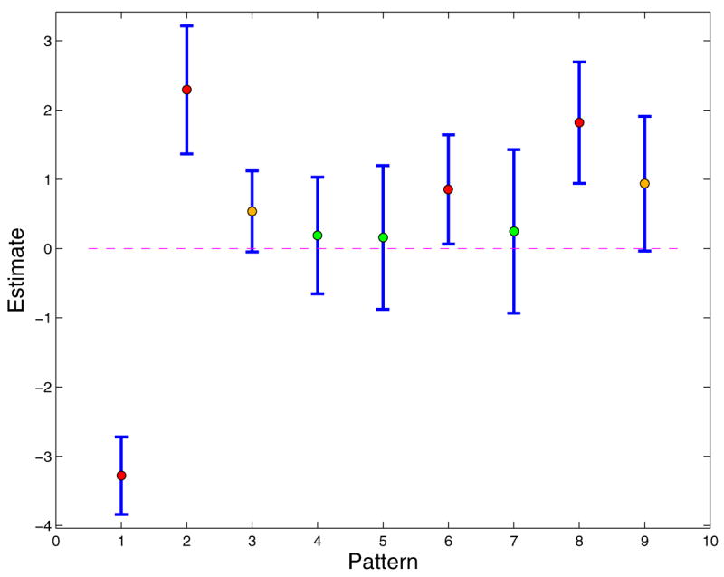
The Eight Patterns that Survived Step 1 of LPS. The Vertical Bars Are 90% Confidence Intervals Based on Linear Logistic Regression. Red Dots Mark the Patterns that Are Significant at the 90% Level. The Orange Dots Are Borderline Cases, the Confidence Intervals Barely Covering 0.
| (11) |
The significance levels for the coefficients of the four patterns in this model (11) can be formally computed and are, respectively 3.3340e-21, 1.7253e-05, 1.5721e-04, and 0.0428. The pattern pky × vtm catches our attention because the pattern effect is strong and both variables are controllable. This model tells us that the distribution of y, myopic change conditional on pky = 1 depends on catct, as well as vtm and higher order interactions, but myopic change conditional on pky = 0 is independent of vtm. This interesting effect can easily be seen by going back to a table of the original catct, pky and vtm data (Table 5). The denominators in the risk column are the number of persons with the given pattern and the numerators are the number of those with y = 1. The first two rows list the heavy smokers with cataract. Heavy smokers who take vitamins have a smaller risk of having myopic change. The third and fourth rows list the heavy smokers without cataract. Again, taking vitamins is protective. The first four rows suggest that taking vitamins in heavy smokers is associated with a reduced risk of getting more myopic. The last four rows list all non-heavy smokers. Apparently taking vitamins does not similarly reduce the risk of becoming more myopic in this population. Actually, it is commonly known that smoking significantly decreases the serum and tissue vitamin level, especially Vitamin C and Vitamin E, for example [8]. Our data suggest a possible reduction in myopic change in persons who smoke who take vitamins. However, our data are observational and subject to uncontrolled confounding. A randomized controlled clinical trial would provide the best evidence of any effect of vitamins on myopic change in smokers.
Table 5.
The Raw Data for Cataract, Smoking and Not Taking Vitamins
| catct | pky | no vitamins | risk |
|---|---|---|---|
| 1 | 1 | 1 | 17/23 = 0.7391 |
| 1 | 1 | 0 | 7/14 = 0.5000 |
| 0 | 1 | 1 | 22/137 = 0.1606 |
| 0 | 1 | 0 | 2/49 = 0.0408 |
| 1 | 0 | 1 | 18/51 = 0.3529 |
| 1 | 0 | 0 | 19/36 = 0.5278 |
| 0 | 0 | 1 | 22/363 = 0.0606 |
| 0 | 0 | 0 | 13/203 = 0.0640 |
Since the model is the result of previous data mining, caution in making significance statements may be in order. To investigate the probability of the overall procedure to generate significant false patterns, we kept the attribute data fixed, randomly scrambled the response data and applied the LPS algorithm on the scrambled data. The procedure was repeated 1000 times, and in all these runs, 1 main effect, 10 second order, 5 third order and just 1 fourth order patterns showed up. We then checked on the raw data. There are 21 people with the pattern sex × inc × jomyop × asa and 9 of them have myopic change. The incidence rate is 0.4286, as compared to the overall rate of 0.137. Note that none of the variables in this pattern are involved with variables in the two lower order patterns catct and pky × vtm so it can be concluded that the incidence rate is contributed only by the pattern effect. People with the other size four pattern sex × inc × catct × asa have an incidence rate of 0.7727 (17 out of 22), which can be compared with the incidence rate of all people with catct, 0.4919.
We also applied Logic regression and SPLR on this data set. Logic selected both catct and pky × vtm but missed the two high order patterns. Instead, it selected asa as a main effect. Note that asa is present in both size four patterns. SPLR selected the same patterns as Logic regression with an addition of pky, which is necessary for pky × vtm to be included. These results agree with what we have found in the simulation studies: they are not as likely as LPS in finding higher order patterns. It is noted that in the original version of LPS [31], Step 1 was tuned by GACV rather than BGACV, and resulted in the above eight patterns in Table 4 plus four more, but the final model after Step 2 was the same.
6. RHEUMATOID ARTHRITIS AND SNPS IN A GENERATIVE MODEL BASED ON GAW 15
Rheumatoid arthritis (RA) is a complex disease with a moderately strong genetic component. Generally females are at a higher risk than males. Many studies have implicated a specific region on chromosome 6 as being related to the risk of RA, recently [7], although possible regions on other chromosomes have also been implicated. The 15th Genetic Analysis Workshop (GAW 15, November 2006 [6]) focused on RA, and an extensive simulation data set of cases and controls with simulated single nucleotide polymorphisms (SNPs) was provided to participants and is now publicly available [24]. SNPs are DNA sequence variations that occur when a single nucleotide in the genome sequence is changed. Many diseases are thought to be associated with SNP changes at multiple sites that may interact, thus it is important to have tools that can ferret out groups of possibly interacting SNPs.
We applied LPS to some of the simulated SNP RA GAW 15 data [30]. This provided an opportunity to apply LPS in a context with large genetic attribute vectors, with a known genetic architecture, as described in [24], and to compare the results against the description of the architecture generating the data. We decided to use the GAW data to build a simulation study where we modified the model that appears in [30] to introduce a third order pattern, and in the process deal with some anomalous minus signs in our fitted model, also observed by others [28]. We then simulated phenotype data from the GAW genotypes and covariates, and can evaluate how well the LPS of this paper reproduces the model generating the data with the third order pattern. This section describes the results.
In the simulated genetic data sets [24] genome wide scans of 9187 SNPs were generated with just a few of the SNPs linked to rheumatoid arthritis, according to the described model architecture. The data simulation was set up to mimic the familial pattern of rheumatoid arthritis including a strong chromosome 6 effect. A large population of nuclear families (two parents and two offspring) was generated. This population contains close to 2 million sibling pairs. From this population, a random sample of 1500 families was selected from among families with two affected offspring and another random sample of 2000 families was selected from among families where no member was affected. A total of 100 independent (replicate) data sets were generated. We randomly picked one offspring from each family in replicate 1 as our data set. As for covariates we take the 674 SNPs in chromosome 6 that were generated as a subset of the genome wide scan data and three environmental variables: age, sex and smoking. We created two dummy variables for each SNP since most of them have three levels: normal, one variant allele and two variant alleles. For environmental variables female gender is treated as a risk factor, smoking is treated as a risk factor and age ≥55 is treated as a risk factor. We first describe a reanalysis of this data using the LPS algorithm of this paper. We began our analysis with a screen step. In this step, each variable is entered into a linear logistic regression model. For SNPs with three levels, both dummy variables are entered into the same model. We fit these models and keep the variables with at least one p-value less than 0.05. The screen step selected 74 variables (72 SNPs plus sex and smoking). We then ran LPS on these 74 variables with q = 2, which generates 10371 basis functions. The final model was
| (12) |
where SNP6_153_1 is SNP number 153 on chromosome 6 with 1 variant allele, SNP6_154_1 is SNP number 154 on chromosome 6 with 1 variant allele, SNP6_162_1 is SNP number 162 on chromosome 6 with 1 variant allele and SNP6_153_2 is SNP number 153 on chromosome 6 with 2 variant alleles. When the analysis in [30] was presented at the GAW 15 workshop in November 2006 the tuning procedure presented here had not been finalized, and both Step 1 and Step 2 were tuned against prediction accuracy using replicate 2 as a tuning set. The model (12) obtained here is exactly the same as [30]. We were pleased to find that the in-sample BGACV tuning here was just as good as having a separate tuning set. It is interesting to note that in this particular problem, tuning for prediction and for model selection apparently led to the same results, although in general this is not necessarily the case.
According to the description [24] of the architecture generating the data the risk of RA is affected by two loci (C and D) on chromosome 6, sex, smoking and a sex by locus C interaction. It turns out that both SNP6_153 and SNP6_154 are very close to locus C on chromosome 6 and SNP6_162 is very close to locus D on chromosome 6. The LPS method picked all important variables without any false positives. The description of the data generation architecture said that there was a strong interaction between sex and locus C. We didn’t pick up a sex by locus C interaction in [30], which was surprising.
We were curious about the apparent counter-intuitive negative coefficients for both SNP6_153 patterns and the SNP6_154_1 pattern, which appear to say that normal alleles are risky and variant alleles are protective. Others also found an anomalous protective effect for SNP6_154 normal alleles [28]. We went back and looked at the raw data for SNP6_153 and SNP6_154 as a check but actually Table 4 of [30] shows that this protective effect is in the simulated data, for whatever reason, and it also shows that this effect is stronger for women than for men. We then recoded the SNP6_153 and SNP6_154 responses to reflect the actual effect of these two variables as can be seen in tables of the simulated data.
Table 6 shows the results. The new fitted model, above the double line, has four main effects and five second order patterns. The estimated coefficients are given in the column headed “Coef”. The sex × SNP6_153 and sex × SNP6_154 are there as expected. Two weak second order patterns involving SNP6_553 and SNP6_490 are fitted, but do not appear to be explained by the simulation architecture. This model resulted from fitting with q = 2. Then the LPS algorithm was run to include all third order patterns (q = 3) of the 74 variables which passed the screen step. This generated 403,594 basis functions. No third order patterns were found, and the fitted model was the same as in the q = 2 case. To see if a third order pattern would be found if it were there, we created a generative model with the four main effects and five second order patterns of Table 1, with their coefficients from the “Coef” column, and added to it a third order pattern sex × SNP6_108_2 × SNP6_334_2 with coefficient 3. The two SNPs in the third order pattern were chosen to be well separated in chromosome 6 from the reported gene loci. LPS did indeed find the third order pattern. The estimated coefficients are found under the column headed “Est”. No noise patterns were found, and the two weak second order patterns in the model were missed. However, the potential for the LPS algorithm to find higher order patterns is clear. Further investigation of the properties of the method in genotype-phenotype scenarios is clearly warranted, taking advantage of the power of the LASSO algorithm to handle a truly large number of unknowns simultaneously. Run time was 4.5 minutes on an AMD Dual-Core 2.8 GHz machine with 64 GB memory. Using multiple runs with clever designs to guarantee that every higher order pattern considered is in at least one run, will allow the analysis of much larger SNP data sets with tolerable computer cost.
Table 6.
Fitted and Simulated Models, See Text for Explanation
| Variable 1 | Level 1 | Variable 2 | Level 2 | Coef | Est | |
|---|---|---|---|---|---|---|
| Main effects | constant | - | - | - | −4.8546 | −4.6002 |
| smoking | - | - | - | 0.8603 | 0.9901 | |
| SNP6_153 | 1 | - | - | 1.8911 | 1.5604 | |
| SNP6_162 | 1 | - | - | 2.2013 | 1.9965 | |
| SNP6_154 | 2 | - | - | 0.7700 | 1.0808 | |
|
| ||||||
| Second order patterns | sex | - | SNP6_153 | 1 | 0.7848 | 0.9984 |
| sex | - | SNP6_154 | 2 | 0.9330 | 0.9464 | |
| SNP6_153 | 2 | SNP6_154 | 2 | 4.5877 | 4.2465 | |
| SNP6_153 | 1 | SNP6_553 | 2 | 0.4021 | 0 | |
| SNP6_154 | 2 | SNP6_490 | 1 | 0.3888 | 0 | |
|
| ||||||
| Added | ||||||
|
| ||||||
| Third order pattern | sex × SNP6_108_2 × SNP6_334_2 | 3 | 2.9106 | |||
7. DISCUSSION
In any problem where there are a large number of highly interacting predictor variables that are or can be reduced to dichotomous values, LPS can be profitably used. If the “risky” direction (with respect to the outcome of interest) is known for all or almost all of the variables, the results are readily interpretable. If the risky direction is coded correctly for all of the variables, the fitted model can be expected to be sparser than that for any other coding. However, if a small number of risky variables are coded in the “wrong” way, this usually can be detected. The method can be used as a preprocessor when there are very many continuous variables in contention, to reduce the number of variables for more detailed nonparametric analysis.
LPS, using the algorithm of Appendix B is efficient. On an Intel Quad-core 2.66 GHz machine with 8GB memory the LPS Steps 1 and 2 can do 90,000 basis functions in 4.5 minutes. On an AMD Dual-Core 2.8 GHz machine with 64 GB memory the algorithm did LPS with 403,594 basis functions in 4.5 minutes. It can do 2,000,000 basis functions in 1.25 hours. On the same AMD machine, problems of the size of the myopia data (128 unknowns) can be solved in a few seconds and the GAW 15 problem data (10371 unknowns) was solved in 1.5 minutes.
A number of considerations enter into the choice of q. If the problem is small and the user is interested in high order patterns, it doesn’t hurt to include all possible patterns; if the problem is about the size of Simulation Example 3, q = 4 might be a good choice; for genomic data the choice of q can be limited by extremely large attribute vectors. In genomic or other data where the existence of a very small number of important higher patterns is suspected, but there are too many candidates to deal with simultaneously, it may be possible to overcome the curse of dimensionality with multiple screening levels and multiple runs. For example, considering say, third or even fourth order patterns, variables could be assigned to doable sized runs so that every candidate triple or quadruple of variables is assigned to at least one run. With our purpose built algorithm, the approach is quite amenable to various flavors of exploratory data mining. When a computing system such as Condor (http://www.cs.wisc.edu/condor/) is available, many runs can compute simultaneously.
Many generalizations are available. Two classes of models where the LASSO-Patternsearch approach can be expected to be useful are the multicategory end points model in [22, 33], where an estimate is desired of the probability of being in class k when there are K possible outcomes; another is the multiple correlated endpoints model in [9]. In this latter model, the correlation structure of the multiple endpoints can be of interest. Another generalization allows the coefficients cℓ to depend on other variables; however, the penalty functional must involve ℓ1 penalties if it is desired to have a convex optimization problem with good sparsity properties with respect to the patterns. In studies with environmental as well as genomic data selected interactions between SNP patterns and continuous covariates can be examined [39]: the numerical algorithm can be used on large collections of basis functions that induce a reasonable design matrix, for example collections including splines, wavelets or radial basis functions.
8. SUMMARY AND CONCLUSIONS
The LASSO-Patternsearch algorithm brings together several known ideas in a novel way, using a tailored tuning and pattern selection procedure and a new purpose built computational algorithm. We have examined the properties of the LPS by analysis of observational data, and simulation studies at a scale similar to the observational data. The results are verified in the simulation studies by examination of the generated “truth”, and in the observational data by selective examination of the observational data directly, and data scrambling to check false alarm rates, with excellent results. The novel computational algorithm allows the examination of a very large number of patterns, and, hence, high order interactions. We believe the LASSO-Patternsearch will be an important addition to the toolkit of the statistical data analyst.
Acknowledgments
Thanks to David Callan for many helpful suggestions and for Appendix D.
APPENDIX A. THE BGACV SCORE
We denote the estimated logit function by fλ(·) and define fλi = fλ(x(i)), for i = 1, …, n. Now define
| (13) |
From [37, 23] the leave-one-out CV is
| (14) |
Here and the approximation in (14) follows upon recalling that .
Denote the objective function in (1)–(4) by Iλ (y, c), let Bij = Bj(x(i)) be the entries of the design matrix B, and for ease of notation denote μ = cNB. Then the objective function can be written
| (15) |
Denote the minimizer of (15) by cλ. We know that the l1 penalty produces sparse solutions. Without loss of generality, we assume that the first s components of cλ are nonzero. When there is a small perturbation ε on the response, we denote the minimizer of Iλ(c, y + ε) by . The 0’s in the solutions are robust against a small perturbation in the response. That is, when ε is small enough, the 0 elements will stay at 0. This can be seen by looking at the KKT conditions when minimizing (15). Therefore, the first s components of are nonzero and the rest are zero. For simplicity, we denote the first s components of c by c* and the first s columns of the design matrix B by B*. Then let be the column vector with i entry fλ(x(i)) based on data y, and let be the same column vector based on data y + ε.
| (16) |
Now we take the first-order Taylor expansion of :
| (17) |
Define
and
By the first-order conditions, the left-hand side and the first term of the right-hand side of (17) are zero. So we have
| (18) |
Combine (16) and (18) we have , where
| (19) |
Now let ε be ; then , where and Hi is the ith column of H. By the Leave-Out-One Lemma (stated below), . Therefore
| (20) |
where hii is the iith entry of H. From the right hand side of (14), the approximate CV score is
| (21) |
The GACV score is obtained from the approximate CV score in (21) by replacing hii by and by . It is not hard to see that tr(W H) = trW1/2 H × W1/2 = s ≡ NB0, the number of basis functions in the model, giving
| (22) |
Adding the weight to the “optimism” part of the GACV score, we obtain the B-type GACV (BGACV):
| (23) |
Lemma A.1 (Leave-Out-One Lemma)
Let the objective function Iλ(y, f) be defined as before. Let be the minimizer of Iλ(y, f) with the i th observation omitted and let be the corresponding probability. For any real number ν, we define the vector z = (y1, …, yi−1,ν, yi+1, −, yn)′. Let hλ(i, ν, ·) be the minimizer of Iλ(z, f); then .
The proof of Lemma A.1 is quite simple and very similar to the proof of the Leave-Out-One-Lemma in [39] so we will omit it here.
We remark that in this paper we have employed the BGACV criterion twice as a stringent model selector under the assumption that the true or the desired model is sparse. Simulation experiments (not shown) suggest that the GACV criterion is preferable if the true model is not sparse and/or the signal is weak. The GACV and the BGACV selections probably bracket the region of interest of λ in most applications.
Comments
A referee has asked how BGACV might be compared to the more familiar . where df is the degrees of freedom in the case of Bernoulli data. The short answer to this question is that an exact expression for df does not, in the usual sense, exist in the case of Bernoulli data. Thus, only a hopefully good approximation to something that plays the role of df in the Bernoulli case can be found. This argument, which is independent of the nature of the estimate fλ of f, is found in Section 2 of [23]. We sketch the main idea. Let KL(λ) = KL(f, fλ) be the Kullback-Liebler distance between the distribution with the true but unknown canonical link f and the distribution with link fλ and let
| (24) |
be the comparative Kullback-Liebler distance. The goal is to find an unbiased estimate of CKL(λ) as a function of λ, which will then be minimized to estimate the λ minimizing the true but unknown CKL. Letting we can write CKL(λ) = OBS (λ) + D(λ). Where . Then . Ye and Wong (1997) show, in exponential families, for any estimate fλ of f
| (25) |
Here Eμi (fλi) is the expectation with respect to yi conditional on the yj, j ≠ i being fixed. (Their proof is reproduced in [23].) Ye and Wong call n times the right hand side of (25) the generalized degrees of freedom (GDF). and it does indeed reduce to the usual trace of the influence matrix in the case of Gaussian data with quadratic penalties. Unbiased estimates of the GDF can be found for Poisson, Gamma, Binomial distribution taking on three or more values, and other distributions, using the results in [14] but Ye and Wong show that no unbiased estimate of the GDF in the Bernoulli case exists. See [36]. Thus, in the absence of a bona fide unbiased risk method of estimating the CKL(λ) the alternative GACV based on leave-one-out to target the CKL has been proposed. Thus, in this paper , say, plays the role of df. Since no exact unbiased estimate for df exists, the issue of the accuracy of the approximations in obtaining D̂ reduces to the issue of to what extent the minimizer of GACV (λ) is a good estimate of the minimizer of the (unobservable) CKL(λ). The GACV for Bernoulli data was first proposed in [37] for RKHS (quadratic) penalty functionals, where simulation results demonstrated the accuracy of this approximation. Further excellent favorable results for a randomized version of the GACV with RKHS penalties were presented in [23]. In [39] the GACV was derived for Bernoulli data with l1 penalties with a nontrivial null space, and favorable results for the randomized version were obtained. The derivation was rather complicated, and a simplified derivation as well as a simpler expression for the result which is possible in the present context are presented above. A recent work involving the LASSO in the Bernoulli case with l1 penalty uses a tuning set to choose the smoothing parameters. SPLR [26] uses tr(B∗′W B∗ + λI∗)−1(B∗′W B∗), where I is the diagonal matrix with all 1’s except in the position of the model constant, as their proxy for df in their BIC-like criteria for model selection after fixing λ. In the light of the Ye and Wong result it is no surprise that an exact definition of df in this case cannot be found in the literature.
APPENDIX B. MINIMIZING THE PENALIZED LOG LIKELIHOOD FUNCTION
The function (1) is not differentiable with respect to the coefficients {cℓ} in the expansion (4), so most software for large-scale continuous optimization cannot be used to minimize it directly. We can however design a specialized algorithm that uses gradient information for the smooth term to form an estimate of the correct active set (that is, the set of components cℓ that are zero at the minimizer of (1)). Some iterations of the algorithm also attempt a Newton-like enhancement to the search direction, computed using the projection of the Hessian of onto the set of nonzero components cℓ. This approach is similar to the two-metric gradient projection approach for bound-constrained minimization, but avoids duplication of variables and allows certain other economies in the implementation.
We give details of our approach by simplifying the notation and expressing the problem as follows:
| (26) |
When T is convex (as in our application), z is optimal for (26) if and only if the following condition holds:
| (27) |
for some vector υ in the subdifferential of ||z||1 (denoted by ∂||z||1), that is,
| (28) |
A measure of near-optimality is given as follows:
| (29) |
We have that δ(z) = 0 if and only if z is optimal.
In the remainder of this section, we describe a simplified version of the algorithm used to solve (26), finishing with an outline of the enhancements that were used to decrease its run time.
The basic (first-order) step at iteration k is obtained by forming a simple model of the objective by expanding around the current iterate zk as follows:
| (30) |
where αk is a positive scalar (whose value is discussed below) and dk is the proposed step. The subproblem (30) is separable in the components of d and therefore trivial to solve in closed form, in O(m) operations. We can examine the solution dk to obtain an estimate of the active set as follows:
| (31) |
We define the “inactive set” estimate to be the complement of the active set estimate, that is,
If the step dk computed from (30) does not yield a decrease in the objective function Tλ, we can increase αk and re-solve (30) to obtain a new dk. This process can be repeated as needed. It can be shown that, provided zk does not satisfy an optimality condition, the dk obtained from (30) will yield Tλ(zk + dk) < Tλ(zk) for αk sufficiently large.
We enhance the step by computing the restriction of the Hessian ∇2T(zk) to the set (denoted by ) and then computing a Newton-like step in the components as follows:
| (32) |
where δk is a small damping parameter that that goes to zero as zk approaches the solution, and captures the gradient of the term ||z||1 at the nonzero components of zk + dk. Specifically, coincides with ∂|| zk + dk||1 on the components . If δk were set to zero, would be the (exact) Newton step for the subspace defined by ; the use of a damping parameter ensures that the step is well defined even when the partial Hessian is singular or nearly singular, as happens with our problems. In our implementation, we choose
| (33) |
where δ(z) is defined in (29).
Because of the special form of T (z) in our case (it is the function defined by (2) and (3)), the Hessian is not expensive to compute once the gradient is known. However, it is dense in general, so considerable savings can be made by evaluating and factoring this matrix on only a reduced subset of the variables, as we do in the scheme described above.
If the partial Newton step calculated above fails to produce a decrease in the objective function Tλ, we reduce its length by a factor γk, to the point where has the same sign as for all . If this modified step also fails to decrease the objective Tλ, we try the first-order step calculated from (30), and take this step if it decreases Tλ. Otherwise, we increase the parameter αk, leave zk unchanged, and proceed to the next iteration.
We summarize the algorithm as follows.
Algorithm B.1
given initial point z0, initial damping α0 > 0, constants tol > 0 and η ∈ (0, 1);
for k = 0, 1, 2, …
if δ(zk) < tol
stop with approximate solution zk;
end
Solve (30) for dk; (∗ first-order step ∗)
Evaluate and ;
Compute from (32); (∗ reduced Newton step ∗)
Set and ;
if Tλ(z+) < min(Tλ(zk + dk), Tλ(zk)) (∗ Newton step successful ∗)
zk+1 ← z+;
else
Choose γk as the largest positive number such that
for all i with ;
(∗ damp the Newton step ∗)
Set and ;
if Tλ(z+) < min(Tλ(zk + dk), Tλ(zk)) (∗ damped Newton step successful ∗)
zk+1 ← z+;
else if Tλ(zk + dk) < Tλ(zk) (∗ first-order step successful; use it if Newton steps have failed ∗)
zk+1 ← zk + dk;
else (∗ unable to find a successful step ∗)
zk+1 ← zk;
end
end
(∗ increase or decrease α depending on success of first-order step ∗)
if Tλ(zk + dk) < Tλ(zk)
αk+1 ← ηαk; (∗ first-order step decreased Tλ, so decrease α ∗)
else
αk+1 → αk/η;
end
end
We conclude by discussing some enhancements to this basic approach that can result in significant improvements to the execution time. Note first that evaluation of the full gradient ∇T(zk), which is needed to compute the first-order step (30) can be quite expensive. Since in most cases the vast majority of components of zk are zero, and will remain so after the next step is taken, we can economize by selecting just a subset of components of ∇T (zk) to evaluate at each step, and allowing just these components of the first-order step d to be nonzero. Specifically, for some chosen constant σ ∈ (0, 1], we select σm components from the index set {1, 2, …, m} at random (using a different random selection at each iteration), and define the working set to be the union of this set with the set of indices i for which . We then evaluate just the components of ∇T(zk) for the indices , and solve (30) subject to the constraint that di = 0 for .
Since δ(zk) cannot be calculated without knowledge of the full gradient ∇T(zk), we define a modified version of this quantity by taking the norm in (29) over the vector defined by , and use this version to compute the damping parameter δk in (33).
We modify the convergence criterion by forcing the full gradient vector to be computed on the next iteration k + 1 when the threshold condition δ(zk) < tol is satisfied. If this condition is satisfied again at iteration k + 1, we declare success and terminate.
A further enhancement is that we compute the second-order enhancement only when the number of components in is small enough to make computation and factorization of the reduced Hessian economical. In the experiments reported here, we compute only the first order step if the number of components in exceeds 500.
APPENDIX C. RESULTS OF SIMULATION EXAMPLE 3
See Table 7.
APPENDIX D. EFFECT OF CODING FLIPS
Proposition
Let f (x) = μ + Σcj1j2..jrBj1j2..jr(x) with all cj1j2..jr which appear in the sum strictly positive. If xj → 1 − xj for j ∈ some subset of {1, 2,…, p} such that at least one xj appears in f, then the resulting representation has at least one negative coefficient and at least as many terms as f. This follows from the
Lemma
Let gk (x) be the function obtained from f by transforming xj →1 − xj, 1 ≤ j ≤ k. Then the coefficient of Bj1j2..jr(x) in gk (x) is
where |·| means number of entries.
Contributor Information
Weiliang Shi, Department of Statistics, University of Wisconsin, 1300 University Avenue, Madison WI 53706, E-mail address: shiw@stat.wisc.edu.
Grace Wahba, Department of Statistics, Department of Computer Science and Department of Biostatistics and Medical Informatics, University of Wisconsin, 1300 University Avenue, Madison WI 53706, E-mail address: wahba@stat.wisc.edu.
Stephen Wright, Department of Computer Science, University of Wisconsin, 1210 West Dayton Street, Madison WI 53706, E-mail address: swright@cs.wisc.edu.
Kristine Lee, Department of Ophthalmology and Visual Science, University of Wisconsin, 610 Walnut St., Madison WI, klee@epi.ophth.wisc.edu.
Ronald Klein, Department of Ophthalmology and Visual Science, University of Wisconsin, 610 Walnut St., Madison WI, kleinr@epi.ophth.wisc.edu.
Barbara Klein, Department of Ophthalmology and Visual Science, University of Wisconsin, 610 Walnut St., Madison WI, kleinb@epi.ophth.wisc.edu.
References
- 1.Breiman L, Friedman J, Olshen R, Stone C. Classification and Regression Trees. Wadsworth: 1984. [Google Scholar]
- 2.Chan K-Y, Loh W-Y. Lotus: An algorithm for building accurate and comprehensible logistic regression trees. Journal of Computational and Graphical Statistics. 2004;13:826–852. [Google Scholar]
- 3.Chen S, Donoho D, Saunders M. SIAM J Sci Comput. Vol. 20. 1998. Atomic decomposition by basis pursuit; pp. 33–61. [Google Scholar]
- 4.Craven P, Wahba G. Smoothing noisy data with spline functions: estimating the correct degree of smoothing by the method of generalized cross-validation. Numer Math. 1979;31:377–403. [Google Scholar]
- 5.Efron B, Hastie T, Johnstone I, Tibshirani R. Least angle regression. Ann Statist. 2004;32:407–499. [Google Scholar]
- 6.Cordell H, et al. Genetic analysis workshop 15: gene expression analysis and approaches to detecting multiple functional loci. BMC Proceedings. 2007;1(Suppl 1 S1):1–4. doi: 10.1186/1753-6561-1-s1-s1. [DOI] [PMC free article] [PubMed] [Google Scholar]
- 7.Thompson W, et al. Rheumatoid arthritis association at 6q23. Nature Genetics. 2007 Nov 4; doi: 10.1038/ng.2007.32. [DOI] [PMC free article] [PubMed] [Google Scholar]
- 8.Galan P, Viteri F, Bertrais S, et al. Serum concentrations of beta-carotene, vitamins C and E, zinc and selenium are influenced by sex, age, diet, smoking status, alcohol consumption and corpulence in a general French adult population. Eur J Clin Nutr. 2005;59:1181–1190. doi: 10.1038/sj.ejcn.1602230. [DOI] [PubMed] [Google Scholar]
- 9.Gao F, Wahba G, Klein R, Klein B. Smoothing spline ANOVA for multivariate Bernoulli observations, with applications to ophthalmology data, with discussion. J Amer Statist Assoc. 2001;96:127–160. [Google Scholar]
- 10.George E. The variable selection problem. J Amer Statist Assoc. 2000;95:1304–1308. [Google Scholar]
- 11.Golub G, Heath M, Wahba G. Generalized cross validation as a method for choosing a good ridge parameter. Technometrics. 1979;21:215–224. [Google Scholar]
- 12.Gunn S, Kandola J. Structural modelling with sparse kernels. Machine Learning. 2002;48:137–163. [Google Scholar]
- 13.Haughton D. On the choice of a model to fit data from an exponential familly. Ann Statist. 1988;16:342–355. [Google Scholar]
- 14.Hudson M. A natural identity for exponential families with applications in multiparameter estimation. Ann Statist. 1978;6:473–484. [Google Scholar]
- 15.Klein R, Klein BEK, Linton K, DeMets D. The Beaver Dam eye study: Visual acuity. Ophthalmology. 1991;98:1310–1315. doi: 10.1016/s0161-6420(91)32137-7. [DOI] [PubMed] [Google Scholar]
- 16.Knight K, Fu W. Asymptotics for LASSO-type estimators. Ann Statist. 2000;28:1356–1378. [Google Scholar]
- 17.Lee K, Klein B, Klein R. Changes in refractive error over a 5-year interval in the Beaver Dam Eye Study. Investigative Ophthalmalogy & Visual Science. 1999;40:1645–1649. [PubMed] [Google Scholar]
- 18.Lee K, Klein B, Klein R, Wong T. Changes in refraction over 10 years in an adult population: the Beaver Dam Eye Study. Investigative Ophthalmology Visual Science. 2002;43:2566–2571. [PubMed] [Google Scholar]
- 19.Lee Y, Kim Y, Lee S, Koo J. Structured multicategory support vector machines with analysis of variance decomposition. Biometrika. 2006;93:555–571. [Google Scholar]
- 20.Leng C, Lin Y, Wahba G. A note on the LASSO and related procedures in model selection. Statistica Sinica. 2006;16:1273–1284. [Google Scholar]
- 21.Li KC. Asymptotic optimality of CL and generalized cross validation in ridge regression with application to spline smoothing. Ann Statist. 1986;14:1101–1112. [Google Scholar]
- 22.Lin X. Technical Report 1003, PhD thesis. Department of Statistics, University of Wisconsin; Madison WI: 1998. Smoothing spline analysis of variance for polychotomous response data. Available via G. Wahba’s website. [Google Scholar]
- 23.Lin X, Wahba G, Xiang D, Gao F, Klein R, Klein B. Smoothing spline ANOVA models for large data sets with Bernoulli observations and the randomized GACV. Ann Statist. 2000;28:1570–1600. [Google Scholar]
- 24.Miller M, Lind G, Li N, Jang S. Genetic analysis workshop 15: Simulation of a complex genetic model for rheumatoid arthritis in nuclear families including a dense snp map with linkage disequilibrium between marker loci and trait loci. BMC Proceedings. 2007;1(Suppl 1 S4):1–7. doi: 10.1186/1753-6561-1-s1-s4. [DOI] [PMC free article] [PubMed] [Google Scholar]
- 25.Osborne M, Presnell B, Turlach B. On the LASSO and its dual. J Comp Graph Stat. 2000;9:319–337. [Google Scholar]
- 26.Park M, Hastie T. Penalized logistic regression for detecting gene interactions. Biostatistics. 2008;9:30–50. doi: 10.1093/biostatistics/kxm010. [DOI] [PubMed] [Google Scholar]
- 27.Ruczinski I, Kooperberg C, LeBlanc M. Logic regression. J Computational and Graphical Statistics. 2003;12:475–511. [Google Scholar]
- 28.Schwartz D, Szymczak S, Ziegler A, Konig R. Picking single-nucleotide polymorphisms in forests. BMC Proceedings. 2007;1(Suppl 1 S59):1–5. doi: 10.1186/1753-6561-1-s1-s59. [DOI] [PMC free article] [PubMed] [Google Scholar]
- 29.Seet B, Wong T, Tan D, Saw S, Balakrishnan V, Lee L, Lim A. Myopia in Singapore: taking a public health approach. Br J Ophthalmol. 2001;85:521–526. doi: 10.1136/bjo.85.5.521. [DOI] [PMC free article] [PubMed] [Google Scholar]
- 30.Shi W, Lee K, Wahba G. Detecting disease-causing genes by LASSO-patternsearch algorithm. BMC Proceedings. 2007;1(Suppl 1 S60):1–5. doi: 10.1186/1753-6561-1-s1-s60. [DOI] [PMC free article] [PubMed] [Google Scholar]
- 31.Shi W, Wahba G, Wright S, Lee K, Klein R, Klein B. LASSO-Patternsearch algorithm with application to ophthalmalogy data. Department of Statistics, University of Wisconsin; Madison WI: 2006. Technical Report 1131. [DOI] [PMC free article] [PubMed] [Google Scholar]
- 32.Tibshirani R. Regression shrinkage and selection via the LASSO. J Roy Stat Soc B. 1996;58:267–288. [Google Scholar]
- 33.Wahba G. Soft and hard classification by reproducing kernel Hilbert space methods. Proceedings of the National Academy of Sciences. 2002;99:16524–16530. doi: 10.1073/pnas.242574899. [DOI] [PMC free article] [PubMed] [Google Scholar]
- 34.Wahba G, Wold S. A completely automatic French curve. Commun Stat. 1975;4:1–17. [Google Scholar]
- 35.Whittaker J. Graphical Models in Applied Mathematical Multivariate Statistics. Wiley; 1990. [Google Scholar]
- 36.Wong W. Estimation of the loss of an estimate. In: Fan J, Koul H, editors. Frontiers of Statistics. Imperial College Press; London: 2006. pp. 491–506. [Google Scholar]
- 37.Xiang D, Wahba G. A generalized approximate cross validation for smoothing splines with non-Gaussian data. Statistica Sinica. 1996;6:675–692. [Google Scholar]
- 38.Zhang H, Lin Y. Component selection and smoothing for nonparametric regression in exponential families. Statistica Sinica. 2006;16:1021–1042. [Google Scholar]
- 39.Zhang H, Wahba G, Lin Y, Voelker M, Ferris M, Klein R, Klein B. Variable selection and model building via likelihood basis pursuit. J Amer Statist Assoc. 2004;99:659–672. [Google Scholar]
- 40.Zou H, Hastie T. Regularization and variable selection via the elastic net. Journal of the Royal Statistical Society: Series B. 2005;67:301–320. [Google Scholar]