Gapped Pulses for Frequency-Swept MRI

Abstract

A recently introduced method called SWIFT (SWeep Imaging with Fourier Transform) is a fundamentally different approach to MRI which is particularly well suited to imaging objects with extremely fast spin-spin relaxation rates. The method exploits a frequency-swept excitation pulse and virtually simultaneous signal acquisition in a time-shared mode. Correlation of the spin system response with the excitation pulse function is used to extract the signals of interest. With SWIFT, image quality is highly dependent on producing uniform and broadband spin excitation. These requirements are satisfied by using frequency-modulated pulses belonging to the hyperbolic secant family (HSn pulses). This article describes the experimental steps needed to properly implement HSn pulses in SWIFT. In addition, properties of HSn pulses in the rapid passage, linear region are investigated, followed by an analysis of the pulses after inserting the “gaps” needed for time-shared excitation and acquisition. Finally, compact expressions are presented to estimate the amplitude and flip angle of the HSn pulses, as well as the relative energy deposited by the SWIFT sequence.

Introduction

Advanced digital electronics of modern NMR instruments, combined with their flexible programming capabilities, have led to unprecedented sophistication in NMR experimentation. In particular, the capabilities provided by waveform synthesis have allowed re-evaluation of ideas and techniques from the past, many of which have been essentially forgotten. One example is the recently described MRI method called SWIFT (SWeep Imaging with Fourier Transformation) [1]. SWIFT is a close relative of the classical experiment called rapid scan correlation spectroscopy [2,3]. SWIFT uses swept radiofrequency (RF) excitation and virtually simultaneous signal acquisition in a time-shared mode, which allows imaging of objects with ultra fast spin-spin relaxation rates. In SWIFT as in rapid scan correlation spectroscopy, correlation of the spin system response with the excitation pulse function is used to extract useful signal.

High quality images can be produced with SWIFT only when the excitation is uniform over a bandwidth equal to the image acquisition bandwidth [1]. Certain types of frequency-modulated (FM) pulses that function according to adiabatic principles offer the capability to produce a broadband and flat excitation profile with low RF amplitude (B₁) [4,5]. Most FM pulses have been created for the purpose of inverting magnetization (i.e. adiabatic full passage (AFP)), but these same pulses can be used to excite lower flip angles, while retaining essentially the same shape of the frequency-response profile. In contrast to adiabatic inversion, accomplishing excitation with lower flip angles requires either decreasing B₁ or increasing the rate at which the time-dependent pulse frequency ω_RF(t) is swept [6]. In doing so, the operating point is changed from the adiabatic region to the region known as the rapid passage, linear region, which satisfies the conditions:

$$a{T}_2^2>>1$$ (1a)

and

$$a>>{({\omega }_1∕2\pi )}^2,$$ (1b)

where a is the frequency acceleration in Hertz per second (i.e., a = (dω_RF/dt)/2π), T₂ is spin-spin relaxation time in units of seconds, and ω₁ is the amplitude of RF field in angular frequency units (i.e., ω₁ = γB₁, where γ is the gyromagnetic ratio).

Unlike rapid scan correlation spectroscopy, SWIFT does not have restrictions on the shape of the RF sweep function [1], and therefore, many different kinds of FM pulses can be used for this application. In SWIFT experiments to date, we have exploited FM pulses belonging to a class of hyperbolic secant pulses known as HSn pulses [7]. In this work, properties of HSn pulses in the rapid passage, linear region are investigated, followed by a further analysis of the pulses after inserting the “gaps” needed for time-shared excitation and acquisition in SWIFT. With the aid of Bloch simulations, a compact expression is obtained which allows the flip angle produced by HSn pulses to be predicted analytically and provides a tool to estimate RF energy, peak amplitude, and relative specific absorption rate (SAR) for the entire SWIFT sequence.

Frequency-modulated pulses of the HSn family

Frequency-modulated HSn pulses were originally developed [7] for the purpose of accomplishing adiabatic inversion (i.e., AFP pulses) with reduced peak amplitude relative to the well known hyperbolic secant (HS) pulse [8]. The RF driving function f_n(t) was chosen to be a modified HS function,

$$f_{\mathrm{n}}\left(t\right)=\mathrm{sech}\left(\beta {(2t∕T_{\mathrm{p}}-1)}^n\right),$$ (2)

where n is a dimensionless shape factor (typically n ≥1), β is a dimensionless truncation factor (usually β ≈ 5.3), and T_p is the pulse length (i.e., 0 ≤ t ≤ T_p). The dimensionless relative integral I(n) and relative power P(n) of the driving function (Eq. [2]) can be obtained, but do not have known analytic closed form expressions when n > 1. For convenience, here approximations will be used which for β ≥ 3 and n ≥ 1 have 3% or better accuracy, such that:

$$I\left(n\right)=\frac{2}{T_{\mathrm{p}}}{\int }_0^{T_{\mathrm{p}}}{f}_{\mathrm{n}}\left(\tau \right)d\tau \approx {\left(\frac{\pi }{2\beta }\right)}^{1∕n}$$ (3a)

$$P\left(n\right)=\frac{2}{T_{\mathrm{p}}}{\int }_0^{T_{\mathrm{p}}}{f_{\mathrm{n}}}^2\left(\tau \right)d\tau \approx {\left(\frac{1}{\beta }\right)}^{1∕n}.$$ (3b)

For n → ∞ the function f_n(t) becomes a rectangle which describes the shape of chirp and square pulses () with corresponding parameters equal to one, i.e., I = P = 1.

In the case of HSn pulses, the time-dependent RF amplitude and angular frequency can be written as,

$${\omega }_1\left(t\right)={\omega }_{1\max }{f}_{\mathrm{n}}\left(t\right),$$ (4a)

$${\omega }_{\mathrm{RF}}\left(t\right)={\omega }_{\mathrm{c}}+2A\left(\frac{{\int }_0^t{f_{\mathrm{n}}}^2\left(\tau \right)d\tau }{{\int }_0^{T_{\mathrm{p}}}{f_{\mathrm{n}}}^2\left(\tau \right)d\tau }-\frac{1}{2}\right),$$ (4b)

respectively, where ω_1max = γB_1max, ω_c is the angular carrier frequency, and A is the amplitude of the frequency modulation. Most modern NMR instruments execute FM pulses by modulating the pulse phase, rather than frequency, according to the function,

$$\varphi \left(t\right)={\int }_0^t({\omega }_{\mathrm{RF}}\left(\tau \right)-{\omega }_{\mathrm{c}})d\tau .$$ (5)

With amplitude and phase modulation, the FM pulse is described by the function

$$x\left(t\right)={\omega }_1\left(t\right)e^{-j\varphi \left(t\right)}.$$ (6)

The excitation profile of HSn pulses

By analyzing the vector motions in a rotating frame of reference [4], the excitation bandwidth produced by an HSn pulse can be understood in terms of a frequency-swept excitation (-A ≤ ω_RF(t) - ω_c) ≤ A). Accordingly, the HSn pulse bandwidth (in Hz) is theoretically given by b_w = A/π. With uniform energy distribution inside the baseband [7,9], the frequency-response profile of the HSn pulse is highly rectangular in shape, with edges becoming sharper with an increasing time-bandwidth product, R = AT_p/π [10].

An appreciation of the features of HSn pulses can be readily obtained by performing Bloch simulations. Fig. 1 shows simulated data using HS1 and chirp pulses (R = 256), and for comparison, the data obtained with a simple square pulse are also shown. Bloch simulations were used to find the bandwidth b_w,95 for which at least 95% of the maximal excitation was achieved [11]. In Fig. 1, b_w,95 is plotted as a function of flip angle θ, after normalizing by b_w,theory, which is defined as the full-width half-maximum bandwidth predicted from linear theory. In other words, b_w,theory = A/π for HSn pulses and b_w,theory = 1/T_p for a square pulse. In Fig. 1 it can be seen that the HS1 and chirp bandwidth is well approximated by the relationship b_w ≈ A/π = R/T_p, for all flip angles (i.e., b_w,95/b_w,theory ≈ 1) In comparison, the excitation bandwidth produced by a square pulse is highly dependent on the choice of flip angle. In the small flip angle region, the bandwidth of the square pulse, as predicted from Fourier analysis under estimates b_w,95 by about a factor of three. Thus, to make a proper comparison with HSn pulses, the square pulse used in the following analysis will have a pulse length T_p = 1/(3b_w), so that it effectively excites the same required bandwidth (b_w,95) as the HSn pulse.

Fig.1.

The dependency of excitation bandwidth on the flip angle for HS1 and chirp pulses with R=256 and for a square pulse. For HS1 and chirp pulses b_w,theory=A/π and for the square pulse b_w,theory=1/T_p. The bandwidth dependence is displayed as the ratio between the Bloch simulations calculated bandwidth needed to achieving 95% maximal excitation and the theoretical values from linear systems considerations.

Characteristics of HSn pulses in the rapid passage, linear region

In the linear region, the flip angle produced by an HSn pulse is a linear function of the RF field strength. The RF field strength expressed in terms of the spectral density at the center frequency (j₀) is

$$j_0=\mid {\int }_0^{T_{\mathrm{p}}}x\left(t\right)dt\mid .$$ (7)

When using amplitude-modulated (AM) pulses without frequency or phase modulation (e.g., a sinc pulse), j₀ is a linear function of T_p according to Eq. [7]. Alternatively, with frequency swept pulses j₀ can be a non-linear function of T_p,, due to the flexibility provided by the additional parameter, R. For example, with a chirp pulse j₀ is inversely proportional to the square root of the frequency acceleration [12]:

$$j_0\propto 1∕\sqrt{a}=\sqrt{\left(\pi T_{\mathrm{p}}\right)∕A}\approx \sqrt{T_{\mathrm{p}}∕b_{\mathrm{w}}}.$$ (8)

As members of the same FM pulse family, HSn pulses are expected to exhibit similar j₀-dependency on a, although with slight differences due to their altered shapes. As shown in Fig. 2, results from Bloch simulations demonstrate how HSn pulses follow these expectations. In Fig. 2, the simulated flip angles (θ) obtained with different settings of the pulse parameters (n, β, T_p, and b_w) are plotted on the ordinate, while the predicted flip angles (θ’) based on the analytical approximation,

$${\theta }^{\prime }={\omega }_{1\max }{\beta }^{-1∕2n}\sqrt{\frac{T_{\mathrm{p}}}{b_{\mathrm{w}}}}\approx j_0,$$ (9a)

are plotted on the abscissa. Here β^-1/2n describes the shape factor, which according to Eq. [3] is related to both the relative integral and power of the pulse as ${\beta }^{-1∕2n}\approx {\left(\frac{\pi }{2}\right)}^{-1∕2n}\sqrt{I\left(n\right)}\approx \sqrt{p\left(n\right)}$ and is equal to 1 in the case of chirp. The approximation θ ≈ θ’ holds for flip angles up to π/2 with an accuracy of about 3%.

Fig. 2.

Flip angles simulated for five HSn pulses with different parameters in the range of changing ω_1max values from 300- 39000 rad/s. The different symbols represent different set of parameters n, β R, and T_p, which are respectively: 1, 7.6, 256, 3 ms (square), 1, 2.99, 256, 3 ms (circle), 1, 5.3 256, 1 ms (up triangle), 1, 5.3 256, 3 ms (down triangle), 8, 5.3, 256, 1 ms (diamond), and chirp with R=256 and T_p =2.56ms (cross). The line represents Eqs. [9a]- [9c].

Alternative equations to approximate the flip angle are

$${\theta }^{\prime }={\omega }_{1\max }{\beta }^{-1∕2n}\frac{T_{\mathrm{p}}}{\sqrt{R}}\approx \theta$$ (9b)

and

$${\theta }^{\prime }={\omega }_{1\max }{\beta }^{-1∕2n}\frac{\sqrt{R}}{b_{\mathrm{w}}}\approx \theta .$$ (9c)

Based on the application, a different choice of dependent versus independent parameters can be made, leading to a requirement for using Eq. [9a], [9b], or [9c]. Many MRI systems implement pulses as a “shape file” requiring fixed R value with the constraint of Eq. [9b] or [9c].

For comparison with the HSn pulses, one can consider a square pulse having approximately the same excitation bandwidth b_w. As described above, when requiring the magnitude of excited magnetization at the edges of the frequency-response profile [11] to be at least 95% of maximum, the pulse length in the linear region must be about $\frac{1}{3b_{\mathrm{w}}}$ (see Fig.1). The flip angle of such a square pulse with peak amplitude ω_1max is equal to

$${\theta }_{\text{square}}=\frac{{\omega }_{1\max }}{3b_{\mathrm{w}}}.$$ (10)

The peak amplitudes needed for excitation to a flip angle θ using HSn and square pulses are

$${\omega }_{1\max }^{\mathrm{HS}\mathit{n}}\approx \theta {\beta }^{1∕2\mathrm{n}}\sqrt{\frac{b_{\mathrm{w}}}{T_{\mathrm{p}}}}=\theta {\beta }^{1∕2\mathrm{n}}\frac{b_{\mathrm{w}}}{\sqrt{R}}$$ (11)

and

$${\omega }_{1\max }^{\mathrm{square}}\approx 3b_{\mathrm{w}}\theta ,$$ (12)

respectively. In contrast to the square pulse, HSn pulses can produce the same θ and b_w values with different settings of the peak RF amplitude, ${\omega }_{1\max }^{\mathrm{HS}\mathit{n}}$. The relative peak amplitude required by the square and HSn pulses is given by the ratio,

$$\frac{{\omega }_{1\max }^{\text{square}}}{{\omega }_{1\max }^{\mathrm{HS}\mathit{n}}}\approx 3{\beta }^{-1∕2\mathrm{n}}\sqrt{R},$$ (13)

which can reach large values, depending on the R value. For example, the HS8 pulse with R = 512 and β = 5.3 has 61 times less peak amplitude than a square pulse exciting the same bandwidth at the same flip angle.

The relative energy, J, radiated by any RF pulse is proportional to the power and duration of the pulse. For an HSn pulse the energy is:

$$J_{\mathrm{HS}\mathit{n}}={\left({\omega }_{1\max }\right)}^{2}p\left(n\right)T_{\mathrm{p}}\approx {\left({\beta }^{1∕2n}\theta \sqrt{\frac{b_{\mathrm{w}}}{T_{\mathrm{p}}}}\right)}^2\frac{T_{\mathrm{p}}}{\sqrt[n]{\beta }}={\theta }^2{b}_{\mathrm{w}}$$ (14)

and accordingly for a square pulse:

$$J_{\text{square}}={\left(3b_{\mathrm{w}}\theta \right)}^2{T}_{\mathrm{p}}=3{\theta }^2{b}_{\mathrm{w}}.$$ (15)

Thus, the radiated RF energy of an HSn pulse is not dependent on n, peak amplitude, or pulse length, and is at least 3 times less than the energy radiated by a square pulse exciting the same bandwidth at the same flip angle.

Generating shaped pulses

To generate a shaped frequency-modulated pulse, the modern NMR spectrometer uses a discrete representation of the pulse with a finite number of pulse elements. One question is, how big must the total number of pulse elements (N_tot) be for proper representation of the pulse? Mathematically such pulse, x’(t), can be represented as the multiplication of the continuous RF pulse function, x(t), by a comb function of spacing Δt (Δt = T_p / N_tot), and convolving the result with a rectangle function having the same width Δt [13]:

$$x^{\prime }\left(t\right)=\left[x\left(t\right)\mathit{comb}(t∕\Delta t)\right]\oplus \mathit{rect}(t∕\Delta t),$$ (16)

where ⊕ is the convolution operation and the comb function is as defined in [14]. The Fourier Transform of x’(t) represents the “low flip angle” excitation profile [15] of the discretized pulse in a frequency (ν) domain,

$$X^{\prime }\left(\nu \right)=B[X\left(\nu \right)\oplus \mathit{comb}\left(\nu \Delta t\right)]\mathit{sinc}\left(\nu \Delta t\right),$$ (17)

where B = Δt² is a scaling factor which will be neglected below for simplicity.

Thus, discretization creates an infinite number of sidebands having the same bandwidth b_w, centered at frequencies k/Δt where k is an integer. The entire excitation spectrum is weighted by the envelope function, $sinc\left(\nu \Delta t\right)=\frac{sin\left(\nu \pi \Delta t\right)}{\nu \pi \Delta t}$. The Nyquist condition for a discretized excitation determines that the sidebands are not aliased when

$$1∕\Delta t\ge b_{\mathrm{w}}.$$ (18)

This in turn determines the minimum number of pulse elements needed to satisfy the Nyquist condition, N_Nyquist, which depends on R according to:

$$N_{\text{Nyquist}}=\frac{T_{\mathrm{p}}}{\Delta t}=\frac{R}{b_{\mathrm{w}}\Delta t}=R.$$ (19)

If the number of pulse elements satisfies the Nyquist condition, then the baseband (-b_w/2≤ν≤b_w/2) can be described by

$$X^{\prime \mathit{main}}\left(\nu \right)=X\left(\nu \right)\mathit{sinc}\left(\nu \Delta t\right).$$ (20)

To reduce the attenuation by sinc (νΔt the length of Δt can be decreased (i.e. the pulse can be oversampled). The parameter used to characterize the level of pulse oversampling is

$$L_{\text{over}}=\frac{N_{\mathrm{tot}}}{N_{\mathrm{Nyquist}}}=\frac{N_{\mathrm{tot}}}{R}.$$ (21)

To meet the requirement that the pulse has at least 95% maximum excitation at the edges of the baseband, L_over must be at least 3, which is similar in form to the constraint in square pulse excitation. In practice it is desirable to use an even larger oversampling level.

The different components of Eq. [17] are presented graphically in Fig. 3 for two different pulse oversampling levels, L_over=1 (Figs. 2a-c) and L_over=8 (Figs. 3f-h). With L_over=1 the resulting excitation spectrum has its first sidebands located immediately adjacent to the baseband (Fig. 3c), and for L_over=8 the first sidebands are pushed outward to center on frequencies ±8b_w (Fig. 3h).

Fig. 3.

Graphical presentation of the components of Eq. [17] (a- c, f- h) and Eq. [24] (d, e, i, j,) for two different pulse oversampling levels L_over=1 (a-e) and L_over=8 (f-j). In the case of the gapped pulse (d, e, i, j), the duty cycle, d_c is equal to 0.5.

Time shared acquisition in gapped HSn pulses

In SWIFT the transmitter is repeatedly turned on and off (every dw interval) to enable sampling “during” the pulse. Such full amplitude modulation of the excitation pulse creates modulation sidebands which have to be considered. If the “transmitter on” time is labeled as τ_p, then the time with the “transmitter off” is equal to dw-τ_p. The pulse is divided into a number of segments (N_seg) each of duration dw, and the total number of sampling points (N_samp) is a multiple of N_seg:

$$N_{\mathrm{samp}}=N_{\mathrm{seg}}{S}_{\text{over}},$$ (22)

where S_over is the integer describing the acquisition oversampling. In general, the parameter N_seg is not dependent on N_tot with only one obvious restriction, N_tot ≥2N_seg. The timing of the gapped HSn pulse as used in SWIFT is presented in Fig. 4a. In the inserts, the detailed structure of the pulse with different pulse oversampling levels (L_over=2 (Fig. 4b) and L_over=6 (Fig. 4c)) is shown. In both examples the pulses have a duty cycle $d_{\mathrm{p}}=\frac{{\tau }_p}{dw}$ equl to 0.5.

Fig. 4.

Shaped pulse with gaps for acquisition in the SWIFT sequence (a) and detailed structure of the pulse with different pulse oversampling levels, L_over=2 (b) and L_over=6 (c). In both examples the duty cycle, d_c is equal to 0.5.

There are different ways to create such segmented pulses based on the same parent pulse (Eq. [6]). One way is to introduce delays with zero amplitudes into the parent pulse (DANTE type) [10] and another involves zeroing pulse elements in the parent pulse (gapped pulse). According to Bloch simulations, the excitation profile of pulses created in these two different ways are the same for R ≤ N_seg / 2. For the same pulse length and duty cycle, the gapped pulse shows better behavior (flatter excitation profile) up to the maximum usable R value, which is R = N_seg (Eq. [19]). For this reason, only gapped pulses are considered here.

Mathematically the gapped pulse can be described as:

$${x^{\prime }}_{\mathrm{gap}}\left(t\right)=x^{\prime }\left(t\right)\left(\mathit{comb}(t∕dw)\oplus \mathit{rect}(t∕{\tau }_{\mathrm{p}})\right).$$ (23)

The Fourier Transform of x’_gap(t) represents the “low flip angle” excitation profile [15] of the gapped pulse:

$${X^{\prime }}_{\text{gap}}\left(\nu \right)=X^{\prime }\left(\nu \right)\oplus [\mathit{comb}\left(\nu dw\right)\mathrm{sinc}\left(\nu {\tau }_{\mathrm{p}}\right)].$$ (24)

The different components of this equation are presented graphically in Fig. 3 for two different levels of pulse oversampling, L_over. Decreasing Δt pushes the sidebands farther from the baseband, but convolution with function comb(νdw)sinc(ντ_p) brings the sidebands back with amplitudes weighted by sinc(m d_c), where m is the sideband order. As a result of this convolution, the baseband’s profile is changed by sideband contamination. Fig. 5 shows profiles of the baseband produced by gapped pulses with two different oversampling levels. Sideband contamination destroys the flatness of the profile, especially at the edges of the baseband. Increasing the level of pulse oversampling helps to decrease or eliminate this effect. This effect becomes negligible with L_over≥16, at which point the baseband and sideband profiles become flat with amplitudes equal to:

$$A_{\mathrm{m}}=sinc\left(m{d}_{\mathrm{c}}\right).$$ (25)

As the duty cycle decreases (d_c→0), the amplitude of sidebands approaches the amplitude of the baseband, whereas the sidebands disappear as d_c→1.

Fig. 5.

Simulated profiles of the baseband for a gapped HS1 pulse (d_c is equal to 0.5) with two different oversampling levels and for a square pulse of $\frac{1}{3b_{\mathrm{w}}}$ duration (a). Zoomed in plots of the top of the baseband are shown in (b).

Characteristics of gapped HSn pulses

The insertion of gaps in an HSn pulse does not change the baseband excitation bandwidth but decreases the flip angle proportionally to the duty cycle. To make the same flip angle, the peak amplitude of the pulse has to be increased, and the resulting energy of the pulse increases by $\frac{1}{d_c}$. Formulas accounting for the duty cycle are given in Table 1.

Table 1.

Properties of gapped HSn and square pulses

Parameter	Gapped HSn pulses (dc-duty cycle)	Square pulse
RF driving function, fn(t)	sech(β(2t/Tp-1)n)	Constant
Relative RF integral, I(n)	$\frac{2d_{\mathrm{c}}}{T_{\mathrm{p}}}{\int }_0^{Tp}{f}_{\mathrm{n}}\left(\tau \right)d\tau \approx d_{\mathrm{c}}{\left(\frac{\pi }{2\beta }\right)}^{1∕n}$	$\underset{n\to \infty }{1}$
Relative RF power, P(n)	$\frac{2d_{\mathrm{c}}}{T_{\mathrm{p}}}{\int }_0^{T\mathrm{p}}{f_{\mathrm{n}}}^2\left(\tau \right)d\tau \approx d_{\mathrm{c}}{\left(\frac{1}{\beta }\right)}^{1∕n}$	$\underset{n\to \infty }{1}$
Total pulse length, Tp, s	$\frac{R}{b_{\mathrm{w}}}$	$\frac{1}{3b_{\mathrm{w}}}$
Amplitude modulation function, ω1(t)	ω1maxfn(t)[comb(bwt)⊕rect(bwdct)]	${\omega }_{1\max }rect(t∕T_{\mathrm{p}})$
Frequency modulation function, ωRF(t) ,rad/s	${\omega }_{\mathrm{c}}+2A\left(\frac{{\int }_0^t{f_{\mathrm{n}}}^2\left(\tau \right)d\tau }{{\int }_0^{T_{\mathrm{p}}}{f_{\mathrm{n}}}^2\left(\tau \right)d\tau }-\frac{1}{2}\right)$	Constant
Flip angle, θ, rad	$\approx {\omega }_{1\max }{d}_{\mathrm{c}}{\beta }^{-1∕2\mathrm{n}}\frac{\sqrt{R}}{b_{\mathrm{w}}}$	$\approx \frac{{\omega }_{1\max }}{3b_{\mathrm{w}}}$
Peak RF amplitude, ω1max, rad/s	$\approx \frac{{\beta }^{1∕2\mathrm{n}}}{d_{\mathrm{c}}\sqrt{R}}\theta b_{\mathrm{w}}$	≈ 3θbw
Relative RF energy, J, rad2/s	$\approx \frac{1}{d_{\mathrm{c}}}{\theta }^2{b}_{\mathrm{w}}$	≈ 3θ2bw
Relative RF energy (Ernst angle), J, rad2/s	$\approx \frac{2T_{\mathrm{R}}{b}_{\mathrm{w}}}{T_1{d}_{\mathrm{c}}}$	$\approx \frac{6T_{\mathrm{R}}{b}_{\mathrm{w}}}{T_1}$
Relative SAR (Ernst angle), SAR, rad2/s2	$\approx \frac{2b_{\mathrm{w}}}{T_1{d}_{\mathrm{c}}}$	$\approx \frac{6b_{\mathrm{w}}}{T_1}$
Relative amplitudes of sidebands, Am	≈ sinc(mdc)	-

Consider the RF energy deposition during an optimized SWIFT sequence. The maximum signal/noise (S/N) ratio is reached when the flip angle is adjusted to the “Ernst angle” (θ_E), which is equal to θ_E = arccos(e^-T_R/T₁), where T_R is repetition time and T₁ is longitudinal relaxation time [16]. An approximation for the Ernst angle in rapid NMR sequences (T_R/T₁<0.1) is:

$${\theta }_{\mathrm{E}}\approx \sqrt{\frac{2T_{\mathrm{R}}}{T_1}}.$$ (26)

In this case, the relative energy deposition according to Eq. [14] is equal to:

$$J_{\mathrm{HS}\mathit{n}}\approx \frac{2T_{\mathrm{R}}{b}_{\mathrm{w}}}{T_1{d}_{\mathrm{c}}},$$ (27)

and the relative SAR for the HSn pulses is:

$${\mathit{SAR}}_{\mathrm{HS}\mathit{n}}\approx \frac{2b_{\mathrm{w}}}{T_1{d}_{\mathrm{c}}},$$ (28)

and for a square pulse is:

$${\mathit{SAR}}_{\text{square}}\approx \frac{6b_{\mathrm{w}}}{T_1}.$$ (29)

Thus, the energy and SAR of a gapped HSn pulse at the Ernst angle is independent of pulse length, R value, and the specific pulse shape (n), and is linearly proportional to pulse baseband width. As compared with a square pulse producing the same bandwidth (b_w,95), HSn pulses have reduced SAR when the duty cycle (d_c) is large and greater SAR when d_c<0.33.

It is worth mentioning that in general, with decreasing pulse duty cycle, the S/N increases together with the SAR, which under certain circumstances means that a compromise in the choice of “optimum” duty cycle must be made. A full analysis of the S/N dependency on duty cycle is beyond the scope of this paper.

Avoidable and unavoidable digitization artifacts in the SWIFT method

In SWIFT useful signal is extracted by correlation of the spin system response with the pulse function. Any misrepresentation of the pulse function will result in a systematic error in the resulting spectrum. Such a systematic error in radial imaging shows up in the reconstructed image as a “bullseye” artifact. To avoid such artifacts, the pulse function used for correlation must be as faithful as possible to the physical pulse transmitted by the RF coil. Some errors can be predicted and neutralized on a software level:

1. Gapping effects. For correlation, instead of the theoretical function, x(t), the discretized function x’_gap(t), must be used.

2. Digitization. The function, x’_gap(t), must be rounded in same way as is done by software and hardware.

3. Timing errors. To avoid temporal rounding error the pulse element duration Δt must be equal to or be a multiple of the minimum time step (temporal resolution) of the waveform generator.

Fig. 5 shows plots of excitation profiles obtained by FT of the pulse functions. Gapped HSn pulses were defined using the digital word lengths permitted by the Varian Inova spectrometer (Palo Alto, CA) used for SWIFT experimentation. Specifically, to create the pulse function x’_gap(t), the amplitude and phase values of the parent HS1 pulse were rounded to 10 and 9 bit length words, respectively. The excitation profiles shown in Fig. 5 exhibit high frequency “noise” (∼0.5% of peak amplitude) which results from rounding amplitude and phase values. Fortunately, by including all discretization constraints in the pulse function before correlation, most of this “noise” contamination can be removed. In our experience, however, the latter procedure removes most, although not all effects from pulse imperfections; therefore, better digital representation of the pulse is desirable. Furthermore, in SWIFT acquisitions using fast repetition of excitation pulses, the complex interplay between the “noisy” profile and the variable recovery of the longitudinal magnetization might lead to additional image artifacts. In this case, correlation will remove only the static part of this “noise”, but the remainder will appear as a “bullseye” artifact in the resulting image. Fortunately, such artifacts can also be reduced during image reconstruction, as will be shown in future publications. Examples of the effects of pulse imperfections on water phantom and human head images are shown on Figs. 6 and 7, respectively. Three-dimensional SWIFT images were reconstructed from frequency-encoded radial projections using gridding [17] without any filtering or other corrections. Fig. 6 presents images and their profiles (horizontal, through the center) of the water phantom acquired with three different levels of oversampling (2,4 and 16). The differences between images are due only to the level of pulse oversampling used. The bullseye artifact decreases with increasing oversampling of the pulse. A similar effect is observed in human head images (Fig. 7). Two datasets were separately acquired corresponding to L_over=2 (upper images) and L_over=32 (bottom images). Selected orthogonal slices are shown. The upper images show a noticeable bullseye artifact, which is almost invisible on the bottom images obtained using the oversampled pulse.

Fig. 6.

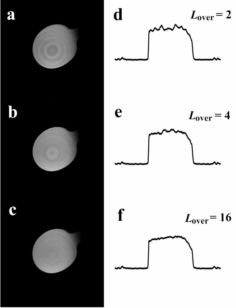
Selected slices of 3D SWIFT images (a,b,c) and their profiles (d,e,f) (horizontal, through center) of a water phantom acquired using HS1 pulse (R = 256, d_c=0.375) with three different levels of pulse oversampling, L_over=2 (a,d), L_over=4 (b,e) and L_over=16 (c,f). Other parameters: diameter of FOV= 3cm, b_w=62.5 kHz, τ_p,=6 μs, θ≈44°, TR= 4.1 ms, N_seg= 256 complex points in radial direction, the total number of radial spokes 16384 (including positive and negative gradient direction), 0.12 mm isotropic voxel size.

Fig. 7.

Selected axial slices of 3D SWIFT images of human brain acquired using HS1 pulse (R = 256, d_c= 0.5) with two different levels of pulse oversampling, L_over=2 (upper images) and L_over=32 (bottom images). Other parameters: diameter of FOV= 40cm, b_w=31 kHz, τ_p = 16 μs, θ ≈ 10°, T_R= 8.5 ms, N_seg= 256 complex points in radial direction, the total number of radial spokes 32000 (including positive and negative gradient direction), 1.6 mm isotropic voxel size and the total acquisition time was 4.5 min.

Discussion and Conclusions

SWIFT is a unique pulse sequence promising to become an important tool in a number of areas, including imaging tissues and materials with extremely fast relaxation rates. Realizing SWIFT’s full potential is currently a challenge, because the technique requires software and hardware capabilities far exceeding typical needs. This article analyzes HSn pulses and considers issues related to their implementation in SWIFT, with particular attention paid to achieving uniform baseband excitation despite the presence of gaps in the pulse waveform.

The first part of this article considered the properties of HSn pulses operated in the rapid passage, linear region. With the aid of Bloch simulations, a set of compact expressions were obtained which can be used to calculate the approximate flip angles produced by an HSn pulse and to estimate critical parameters such as peak amplitude and relative RF energy deposition. It was shown that the efficiency of HSn pulses does not depend on the shape factor (n), pulse length, and peak amplitude. Because a given bandwidth can be excited in many different ways, HSn pulses offer a flexible tool for interrogating spin systems. For example, in a manner similar to that recently demonstrated using AFP pulses [18,19], it may be possible to alter image contrast by collecting images with different pulse parameters.

The second part of this article considered theoretical and experimental aspects of time-shared sweep excitation and acquisition in the SWIFT method. Discretization of pulses and the introduction of gaps in the pulses produce additional sidebands which can contaminate and destroy the flatness of the baseband excitation profile, as well as introduce systematic noise in the acquired data. It was shown that this effect can be minimized by using both pulse oversampling and using the proper pulse function for correlation with the response of the spin system.

In conclusion, SWIFT can be implemented on modern NMR instruments, but the technique demands particular care in the design and implementation of the FM pulses. Although not discussed in detail here, further advances in hardware (eg, improved digital definition of the RF waveform and increased speed of transceiver switching) will also benefit the SWIFT technique.

References

- [1].Idiyatullin D, Corum C, Park J-Y, Garwood M. Fast and quiet MRI using a swept radiofrequency. J. Magn. Reson. 2006;181:342–349. doi: 10.1016/j.jmr.2006.05.014. [DOI] [PubMed] [Google Scholar]
- [2].Dadok J, Sprecher RF. Correlation NMR spectroscopy. J. Magn. Reson. 1974;13:243–248. [Google Scholar]
- [3].Gupta RK, Ferretti JA, Becker ED. Rapid scan Fourier transform NMR spectroscopy. J. Magn. Reson. 1974;13:275–290. [Google Scholar]
- [4].Garwood M, DelaBarre L. The return of the frequency sweep: Designing adiabatic pulses for contemporary NMR. J. Magn. Reson. 2001;153:155–177. doi: 10.1006/jmre.2001.2340. [DOI] [PubMed] [Google Scholar]
- [5].Norris DG. Adiabatic radiofrequency pulse forms in biomedical nuclear magnetic resonance. Concepts Magn. Reson. 2002;14:89–101. [Google Scholar]
- [6].Ernst RR. Sensitivity enhancement in magnetic resonance. Adv. Magn. Reson. 1966;2:1–135. [Google Scholar]
- [7].Tannus A, Garwood M. Improved performance of frequency-swept pulses using offset-independent adiabaticity. J. Magn. Reson. A. 1996;120:133–137. [Google Scholar]
- [8].Silver MS, Joseph RI, Hoult DI. Selective spin inversion in nuclear magnetic resonance and coherent optics through an exact solution of the Bloch-Riccati equation. Phys. Rev. A. 1985;31:2753–2755. doi: 10.1103/physreva.31.2753. [DOI] [PubMed] [Google Scholar]
- [9].Tannus A, Garwood M. Adiabatic pulses. NMR Biomed. 1997;10:423–434. doi: 10.1002/(sici)1099-1492(199712)10:8<423::aid-nbm488>3.0.co;2-x. [DOI] [PubMed] [Google Scholar]
- [10].Ke Y, Schupp DG, Garwood M. Adiabatic DANTE sequences for B1-insensitive narrowband inversion. J. Magn. Reson. 1992;96:663–669. [Google Scholar]
- [11].Bohlen JM, Bodenhausen G. Experimental aspects of chirp NMR spectroscopy. J. Magn. Reson. A. 1993;102:293–301. [Google Scholar]
- [12].Kunz D. Use of frequency-modulated radiofrequency pulses in MR imaging experiments. Magn. Reson. Med. 1986;3:377–84. doi: 10.1002/mrm.1910030303. [DOI] [PubMed] [Google Scholar]
- [13].Barrett H, Myers K. Foundations of image science. John Wiley & Sons; Hoboken, New Jersey: 2004. H. [Google Scholar]
- [14].Gaskill JD. Linear systems, Fourier transforms, and optics. John Wiley and Sons Inc.; New York: 1978. [Google Scholar]
- [15].Pauly J, Nishimura D, Macovski A. A k-space analysis of small-tip-angle excitation. J. Magn. Reson. 1989;81:43–56. doi: 10.1016/j.jmr.2011.09.023. [DOI] [PubMed] [Google Scholar]
- [16].Ernst RR, Anderson WA. Application of Fourier transform spectroscopy to magnetic resonance. Rev. Sci. Instrum. 1966;37:93–102. [Google Scholar]
- [17].Jackson JI, Meyer CH, Nishimura DG, Macovski A. Selection of a convolution function for Fourier inversion using gridding. IEEE Trans. Med. Imaging. 1991;10:473–478. doi: 10.1109/42.97598. [DOI] [PubMed] [Google Scholar]
- [18].Michaeli S, Grohn H, Grohn O, Sorce DJ, Kauppinen R, Springer CS, Jr., Ugurbil K, Garwood M. Exchange-influenced T2rho contrast in human brain images measured with adiabatic radio frequency pulses. Magn. Reson. Med. 2005;53:823–9. doi: 10.1002/mrm.20428. [DOI] [PubMed] [Google Scholar]
- [19].Michaeli S, Sorce DJ, Springer CS, Jr., Ugurbil K, Garwood M. T1rho MRI contrast in the human brain: Modulation of the longitudinal rotating frame relaxation shutter-speed during an adiabatic RF pulse. J. Magn. Reson. 2006;181:135–47. doi: 10.1016/j.jmr.2006.04.002. [DOI] [PubMed] [Google Scholar]