Creating Protein Models from Electron-Density Maps using Particle-Filtering Methods

Abstract

Motivation

One bottleneck in high-throughput protein crystallography is interpreting an electron-density map; that is, fitting a molecular model to the 3D picture crystallography produces. Previously, we developed Acmi, an algorithm that uses a probabilistic model to infer an accurate protein backbone layout. Here we use a sampling method known as particle filtering to produce a set of all-atom protein models. We use the output of Acmi to guide the particle filter's sampling, producing an accurate, physically feasible set of structures.

Results

We test our algorithm on ten poor-quality experimental density maps. We show that particle filtering produces accurate all-atom models, resulting in fewer chains, lower sidechain RMS error, and reduced R factor, compared to simply placing the best-matching sidechains on Acmi's trace. We show that our approach produces a more accurate model than three leading methods – Textal, Resolve, and ARP/wARP – in terms of main chain completeness, sidechain identification, and crystallographic R factor.

1 Introduction

Knowledge of the spatial arrangement of constituent atoms in a complex biomolecules, such as proteins, is vital for understanding their function. X-ray crystallography is the primary technique for determination of atomic positions, or the structure, of biomolecules. A beam of X-rays is diffracted by a crystal, resulting in a set of reflections that contain information about the molecular structure in the form of the electron-density map. Interpretation of these maps requires locating the atoms in complex three-dimensional images. This is a difficult, time-consuming process, that may require weeks or months of an expert crystallographer's time to manually place atoms in the electron density.

Our previous work (DiMaio et al., 2006) developed the automatic interpretation tool Acmi (Automatic Crystallographic Map Interpreter). Acmi employs probabilistic inference to compute a probability distribution of the coordinates of each amino acid, given the electron-density map. However, Acmi makes several simplifications, such as reducing each amino acid to a single atom and confining the locations to a coarse grid. In this work we introduce the use of a statistical sampling method called particle filtering (PF) (Doucet et al., 2000) to construct all-atom protein models, by stepwise extention of a set of incomplete models drawn from a distribution computed by Acmi. This results in a set of probability-weighted all-atom protein models. The method interprets the density map by generating a number of distinct protein conformations consistent with the data. We compare the single model that best matches the density map (without knowing the true solution) with the output of existing automated methods, on multiple sets of crystallographic data which required considerable human effort to solve. We also show that modeling the data with a set of structures, obtained from several particle-filtering runs, results in a better fit than using one structure from a single particle-filtering run. Particle filtering enables the automated building of detailed atomic models for challenging protein crystal data, with a more realistic representation of conformational variation in the crystal.

2 Problem Overview and Related Work

In recent years, considerable investment into structural genomics (i.e. high-throughput determination of protein structures) has yielded a wealth of new data (Berman & Westbrook, 2004; Chandonia & Brenner, 2006). The demand for rapid structure solution is growing, and automated methods are being deployed at all stages of the structural determination process. These new technologies include cell-free methods for protein production (Sawasaki et al., 2002), the use of robotics to enable massive arrays of crystallization conditions (Snell et al., 2004), and new software for automated building of macromolecular models based on the electron-density map (DiMaio et al., 2006; Morris et al., 2003; Ioerger & Sacchettini, 2003; Terwilliger, 2002; Cowtan, 2006). The last problem is addressed in this study.

2.1 Density-map interpretation

A beam of X-rays scattered by a crystalline lattice produces a pattern of reflections, which are measured by a detector. Given complete information, i.e., both the amplitudes and the phases of the reflected photons, one can reconstruct the electron-density map as the Fourier transform of these complex-valued reflections. However, the detector can only measure the intensities of the reflections and not the phases. Thus a fundamental problem of crystallography lies in approximating the unknown phases. Our aim is the construction of an all-atom protein model that best fits a given electron-density map based on approximate phasing.

The electron-density map is defined on a three-dimensional grid of points covering the unit cell, which is the basic repeating unit in the protein crystal. A crystallographer, given the the amino-acid sequence of the protein, attempts to place the amino acids in the unit cell, based on the shape of the electron-density contours. Figure 1 shows the electron-density map as an isocontoured surface. This figure also shows two models of atomic positions consistent with the electron density, where sticks indicate bonds between atoms.

Fig. 1.

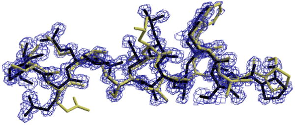
An overview of density-map interpretation. The density map is illustrated with contours enclosing regions of higher density; the protein model uses sticks to indicate bonds between atoms. This figure shows two protein models fit to the density map, one darker and one lighter.

The quality of an electron-density map is limited by its resolution, which measures the interplanar distance between planes corresponding to the highest-frequency reflection. The highest resolution for a data set depends on the order in the crystalline packing, the detector sensitivity, and the brightness of the X-ray source. Figure 2 illustrates the electron density around a tryptophan sidechain at varying resolution, with “ideal” phases computed from a complete all-atom model. Note that at 1 Å resolution, the spheres of individual atoms are clearly visible, while at 4 Å even the overall shape of the tryptophan sidechain is distorted. Typical resolution for protein structures lies in the 2 – 3 Å range.

Fig. 2.

The effect of varying resolution on electron density of a tryptophan sidechain, with phases computed from a final atomic model. The effects of phase error are similar to worsening the resolution.

Another factor that affects the quality of an electron-density map is the accuracy of the computed phases. To obtain an initial approximation of the phases, crystallographers use techniques based on the special features in X-ray scattering produced by heavy atoms, such as multiple-wavelength or single-wavelength anomalous diffraction (MAD or SAD) and multiple isomorphous replacement (MIR). This allows the computation of an initial electron-density map, but its quality can vary greatly depending on the fidelity of the initial phasing. Artifacts produced by phase error are similar to those of worsening resolution; additionally, high spatial frequency noise is also present. The interpretation of a poorly phased map can be very difficult even for a trained expert.

2.2 Acmi's probabilistic protein backbone tracing

We previously developed a method, Acmi, that produces high-confidence backbone traces from poor-quality maps. Given a density map and the protein's amino-acid sequence, Acmi constructs a probabilistic model of the location of each Cα. Statistical inference on this model gives the most probable backbone trace of the given sequence in the density map.

Acmi models a protein using an pairwise Markov field. As illustrated in Figure 3, this approach defines the probability distribution of a set of variables on an undirected graph. Each vertex in the graph is associated with one or more variables, and the probability of some setting of these variables is the product of potential functions associated with vertices and edges in the graph.

Fig. 3.

A sample undirected graphical model corresponding to some protein. The probability of some backbone model is proportional to the product of potential functions: one associated with each vertex, and one with each edge in the fully connected graph.

In Acmi's protein model, vertices correspond to individual amino-acid residues, and the variables associated with each vertex correspond to an amino acid's Cα location and orientation. The vertex potential ψ_i at each node i can be thought of as a “prior probability” on each alpha carbon's location given the density map and ignoring the locations of other amino acids. In this model, the probability of some backbone conformation B = {b₁, … , b_N}, given density map M is given as

$$P(\text{B}|\text{M})=\prod _{\text{amino-acid}i}{\psi }_i(b_i|\text{M})\times \prod _{\text{amino-acid}i,j}{\psi }_{ij}(b_i,b_j)$$ (1)

Acmi's ψ_i considers a 5-mer (5-amino-acid sequence) centered at each position in the protein sequence, and searches a non-redundant subset of the Protein Data Bank (PDB) (Wang & Dunbrack, 2003) for observed conformations of that 5-mer. An improvement to our original approach (DiMaio et al., 2007) uses spherical harmonic decomposition to rapidly search over all rotations of each of these conformations at each location (x, y, z) in the density map.

The edge potentials ψ_ij associated with each edge model global spatial constraints on the protein. Acmi defines two types of edge potentials: adjacency constraints ψ_adj model interactions between adjacent residues (in the primary sequence), while occupancy constraints ψ_occ model interactions between residues distant on the protein chain (though not necessarily spatially distant in the folded structure). Adjacency constraints make sure that Cα's of adjacent amino acids are about 3.8 Å apart; occupancy constraints make sure no two amino acids occupy the same 3D space.

A fast approximate-inference algorithm finds likely locations of each Cα, given the vertex and edge potentials. For each amino acid in the provided protein sequence, Acmi's inference algorithm returns the marginal distribution of that amino acid's Cα location: that is, the probability distribution taking into account the position of all other amino acids. Our previous work shows that Acmi produces more accurate backbone traces than alternative approaches (DiMaio et al., 2006). It also is not as prone to missing pieces in the model, because locations of amino acids not visible in the density map are inferred from the locations of neighboring residues.

2.3 Other approaches

Several methods have been developed to automatically interpret electron-density maps. Given high-quality data (up to about 2.3 Å resolution), one widely used algorithm is ARP/wARP (Morris et al., 2003). This atom-based method heuristically places atoms in the map, connects them, and refines their positions. To handle poor phasing, ARP/wARP is iterative, consisting of alternating steps in which (a) a model is built from a density map, and (b) the map is improved using the model's phases.

Other methods have been developed to handle low-resolution density maps, where atom-based approaches like ARP/wARP fail to produce a reasonable model. Ioerger's Textal (Ioerger & Sacchettini, 2003) and Capra (Ioerger & Sacchettini, 2002) interpret poor-resolution density maps using ideas from pattern recognition. Given a sphere of density from an uninterpreted density map, both employ a set of rotation-invariant statistical features to aid in interpretation. Capra uses a trained neural network to identify Cα. locations. Textal performs a rotational search to place sidechains, using the rotation-invariant features to identify sidechain types. Resolve's automated model-building routine (Terwilliger, 2002) uses a hierarchical procedure in which helices and strands are located by an exhaustive search. High-scoring matches are extended iteratively using a library of tripeptides; these growing chains are merged using a heuristic. Buccaneer (Cowtan, 2006) is a new algorithm that uses an orientation-dependent target function, based on local density agreement, to generate likely Cα. positions and orientations; chains are grown from these “seed” positions, using dihedral angle geometry. Currently, Cowtan's algorithm only constructs a main chain trace.

At lower resolution and with greater phase error, these methods have difficulty in chain tracing and especially in correctly identifying amino acids. Unlike Acmi's model-based approach, they first build a backbone model, then align the protein sequence to it. At low resolutions, this alignment often fails, resulting in the inability to correctly identify sidechain types. These approaches have a tendency to produce disjointed chains in poor-resolution maps, which requires significant human labor to repair.

3 Methods

For each amino acid i, Acmi's probabilistic inference returns the marginal probability distribution p̂_i(b_i) of that amino acid's Cα position. Previously, we computed the backbone trace B = {b₁, …, b_N} (where b_i describes the position and rotation of amino-acid i) as the position of each Cα that maximized Acmi's belief,

$$\begin{array}{c}{b}_i^{\ast }=\text{arg max}{\widehat{p}}_i(b_i)\\ b_i\end{array}$$ (2)

One obvious shortcoming in this previous approach is that biologists are interested in not just the position $b_i^{\ast }$ of each Cα, but in the location of every (non-hydrogen) atom in the protein. Naïvely, we could take Acmi's most-probable backbone model, and simply attach the best-matching sidechain from a library of conformations to each of the model's Cα positions. In Section 4 we show that such a method works reasonably well. Another issue is that the marginal distributions are computed on a grid, which may lead to nonphysical distances between residues when Cα 's are placed on the nearest grid points. Additionally, Acmi's inference is approximate, and errors due to these approximations may produce an incorrect backbone trace, with two adjacent residues located on opposite sides of the map.

Another problem deals with using a “maximum-marginal backbone trace,” that is, independently selecting the position of each residue to maximize the marginal. A density map that contains a mixture of (physically-feasible) protein conformations may have a maximum-marginal conformation that is physically unrealistic. Representing each amino acid's position as a distribution over the map is very expressive. Simply returning the Cα position that maximizes the marginal ignores a lot of information. This section details the application of particle filtering to “explain” the density map using multiple, physically feasible models.

3.1 Particle-filtering overview

We will use a particle-filtering method called statistical importance resampling (SIR) (Doucet et al., 2000; Arulampalam et al., 2001), which approximates the posterior probability distribution of a state sequence x_1:K= {x₁, … , x_K} given observations y_1:K as the weighted sum of finite number of point estimates $x_{1:K}^{(i)}$,

$$p(x_{1:K}|y_{1:K})\approx \sum _{i=1}^N{w}_i\delta (x_{1:K}-x_{1:K}^{(i)})$$ (3)

Here, i is the particle index, w_i is particle i's weight, K is the number of states (here the number of amino acids), and δ is the Dirac delta function. In our application, x_k describes the position of every non-hydrogen atom in amino acid k; y_k is a 3D region of density in the map.

In our work, the technical term “particle” refers to one specific 3D layout of all the non-hydrogen atoms in a contiguous subsequence of the protein (e.g., from amino acid 21 to 25). PF represents the distribution of some subsequence's layout using a set of distinct layouts for that subsequence (in other words, what we are doing is illustrated in Figure 1, where each protein model is a single particle).

At each iteration of particle filtering, we advance the extent of each particle by one amino acid. For example, given x_21:25 = {x₂₁, … .x₂₅} the position of all atoms in amino acids 21 through 25 (we will use this shorthand notation for a particle throughout the paper), PF samples the position of the next amino acid, in this case x₂₆. Ideally, particle filtering would sample these positions from the posterior distribution: the probability of x₂₆'s layout given the current particle and the map. SIR is based on the assumption that this posterior is difficult to sample directly, but easy to evaluate (up to proportionality). Given some other function (called the importance function) that approximates the posterior, particle filtering samples from this function instead, then uses the ratio of the posterior to the importance function to reweight the particles.

To give an example of an importance function, particle-filtering applications often use the prior conditional distribution p(x_k|x_k−1) as the importance function. After sampling the data, y_k will be used to weight each particle. In our application, this is analogous to placing an amino acid's atoms using only the layout of the previous amino acid, then reweighting by how well it fits the density map.

We use a particle resampling step to address the problem of degeneracy in the particle ensemble (Kong et al., 1994). As particles are extended, the variance of particle weights tends to increase, until there are few particles with non-negligible weights, and much effort is spent updating particles with little or no weight. To ameliorate this problem, an optional resampling step samples (with replacement) a new set of N particles at each iteration, with the probability of selecting a particle proportional to its weight. This ensures most particles remain on high-likelihood trajectories in state space.

What makes SIR (and particle filtering methods in general) different from Markov-chain Monte Carlo (MCMC) is that MCMC is concerned with the stationary distribution of the Markov chain. In particle filtering, one is not concerned with convergence of the point estimates, rather, the distribution is simply modeled by the ensemble of particles, whether or not they converge.

3.2 Protein particle model

An overview of our entire algorithm appears in Algorithm 1. For density-map interpretation, we use the variable x_k to denote the position of every atom in amino-acid k. We want to find the complete (all-atom) protein model x_1:K that best explains the observed electron-density map y. To simplify, we parameterize x_k as a Cα location b_k (the same as b_i in Equation 2), and a sidechain placement s_k. The sidechain placement identifies the 3D location of every non-hydrogen sidechain atom in amino-acid k, as well as the position of backbone atoms C, N, and O.

Algorithm 1: Acmi-PF's algorithm for growing a protein model.

input : density map y, amino-acid marginals p̂k(bk)

output: set of protein models $x_{1:K}^{(i)}$ and weights $w_K^{(i)}$

// start at some AA with high certainty about its location

choose k such that p̂k( $b_k^{(i)}$) has minimum entropy

foreach particle i = 1… N do

choose $b_k^{(i)}$ at random from p̂k( $b_k^{(i)}$)

$w_k^{(i)}$ ← 1/N

end

foreach residue k do

foreach particle i = 1… N do

// choose bk+1 (or bk−1) given $b_k^{(i)}$

{ $b_{k+1}^{\ast m}$ } ← choose M samples from φadj( $b_k^{(i)}$, bk+1)

w*m ← belief p̂i ( $b_{k+1}^{\ast m}$)

$b_{k+1}^{\left(i\right)}$ ← choose $b_{k+1}^{\ast m}$ with probability ∝ w*m

$w_{k+1}^{\left(i\right)}$ ← $w_k^{\left(i\right)}$ · ${\sum }_{m=1}^M$ w*m

// choose skgiven $b_{k-1:k+1}^{(i)}$

{ $s_k^{\ast l}$} ← sidechain conformations for amino-acid k

$p_{\text{null}}^{\ast l}$ ← prob cc( $s_k^{\ast l}$, EDM[bk]) occurred by chance

sk ← choose $s_k^{\ast l}$ with probability ∝ 1/ $p_{\text{null}}^{\ast l}$ − 1

$w_{k+1}^{\left(i\right)}$ ← $w_k^{\left(i\right)}$ · ${\sum }_{l=1}^L$ 1/ $p_{\text{null}}^{\ast l}$ −1

end

end

Given this parameterization, the Markov process alternates between placing: (a) Cα positions and (b) sidechain atoms. That is, an iteration of particle filtering first samples b_k+1 (Cα of amino-acid k + 1) given b_k, or alternatively, growing our particle toward the N-terminus would sample b_k−1 given b_k. Then, given the triple b_k−1:k+1, we sample sidechain conformation s_k.

3.2.1 Using Acmi-computed marginals to place Cα's

In our algorithm's backbone step we want to sample the Cα position b_k+1 (or b_j−1), given our growing trace $b_{j:k^{,}}^{(i)}$, for each particle i. That is, we want to define our sampling function $q(b_{k+1}|b_j^{(i)},\mathrm{\dots },b_k^{(i)},\text{y})$. Doucet et al. (2000) defines the optimal sampling function as the conditional marginal distribution

$$q(b_{k+1}|b_j^{(i)},\dots ,b_k^{(i)},\text{y})=p(b_{k+1}|b_k^{(i)},\text{y})$$ (4)

While it is intractable to compute Equation 4 exactly, it is straightforward to estimate using Acmi's Markov-field model

$$\begin{array}{c}p(b_{k+1}|b_k^{\left(i\right)},y_k)\propto p(b_k^{\left(i\right)},b_{k+1}|\text{y})/p(b_k^{\left(i\right)}|\text{y})\\ \hfill ={\widehat{p}}_{k+1}(b_{k+1})\cdot {\psi }_{\text{adj}}(b_k^{\left(i\right)},b_{k+1})\end{array}$$ (5)

Here, p̂_k+1(b_k+1) is the Acmi-computed marginal distribution for amino-acid k + 1 (p̂_k+1's dependence on y dropped for clarity). We sample Cα k + 1's location from the product of (a) k + 1's marginal distribution and (b) the adjacency potential between Cα k and Cα k + 1.

The optimal sampling function has a corresponding weight update

$$w_{k+1}^i\propto w_k^i\times \int p(y_{k+1}|b_{k+1},b_k^{(i)})d{b}_k$$ (6)

This integral, too, is intractable to compute exactly, but can be approximated using Acmi's marginals

$$w_{k+1}^i\propto w_k^i\times {\int \widehat{p}}_{k+1}(b_{k+1})\cdot {\psi }_{\text{adj}}(b_k^{(i)},b_{k+1})d{b}_k$$ (7)

Equations 5 and 7 suggest a sampling approach to the problem of choosing location of Cα k +1 and reweighting each particle. This sampling approach, shown in Algorithm 1, is illustrated pictorially in Figure 4.

Fig. 4.

An overview of the backbone forward-sampling step. Given positions b_k−1 and b_k, we sample M positions for b_k−1 using the empirically-derived distribution of Cα–Cα–Cα pseudoangles. Each potential b_k+1 is weighted by the belief $\widehat{p}(b_{k+1}^{\ast m}|\text{y})$. We choose a single location from this distribution; the particle weight is multiplied by the sum of these weights in order to approximate Equation 6.

We sample M potential Cα locations from ${\psi }_{\text{adj}}(b_k^{(i)},b_{k+1})$, the adjacency potential between k and k + 1, which models the allowable conformations between two adjacent Cα's. We assign each sample a weight: the approximate marginal probability p̂_k+1 at each of these sampled locations. We select a sample from this weighted distribution, approximating Equation 5. Finally, we reweight our particle as the sum of weights of all the samples we considered. This sum approximates the integral in Equation 7.

This process, in which we consider M potential Cα locations, is repeated for every particle in the particle filter for each Cα in the protein. For every particle, we begin by sampling locations for the amino-acid k whose marginal distribution has the lowest entropy (we use a soft-minimum to introduce randomness in the order in which amino acids are placed). This corresponds to the amino acid which Acmi is most sure of the location. The direction we sample at each iteration (i.e. toward the N- or C-terminus) is also decided by the entropy of the marginal distributions.

3.2.2 Using sidechain templates to sample sidechains

Once our particle filter has placed Cα's k − 1, k, and k+ 1 at 3D locations $b_{k-1:k+1}^{(i)}$, it is ready to place all the sidechain atoms in amino-acid k. We denote the position of these sidechain atoms s_k. Given the primary amino-acid sequence around k, we consider all previously observed conformations (i.e., those in the PDB) of sidechain k. Thus, s_k consists of (a) an index into a database of known sidechain 3D structures and (b) a rotation.

To further simplify, each sidechain template models the position of every atom from Cα^k−1 to Cα^k+1. Then, given three consecutive backbone positions $b_{k-1:k+1}^{(i)}$, the orientation of sidechain s_k is determined by aligning the three Cα's in the sidechain template to $b_{k-1:k+1}^{(i)}$.

As Algorithm 1 shows, sidechain placement is quite similar to the Cα placement in the previous section. One key difference is that sidechain placement cannot take advantage of Acmi's marginal distribution, as Acmi's probability distributions have marginalized away sidechain conformations. Instead, the probability of a sidechain is calculated on-the-fly using the cross-correlation between a potential conformation's density and a region around b_k in the density map.

Figure 5 illustrates the process of choosing a sidechain conformation for a single particle i. We consider each of L different sidechain conformations for amino-acid k. For each sidechain conformation $s_k^{\ast l},l\in \{1,\dots ,L\}$ we compute the correlation coefficient between the conformation and the map

Fig. 5.

An overview of the sidechain sampling step. Given positions b_k−1:k+1, we consider L sidechain conformations $s_k^{\ast l}$. Each potential conformation is weighted by the probability of the map given the sidechain conformation, as given in Equation 9. We choose a sidechain from this distribution; the particle weight is multiplied by the sum of these weights.

$$C{C}^l=\text{cross-correlation}(s_k^{\ast l},\text{EDM}[b_k^{(i)}])$$

EDM[b_k] denotes a region of density in the neighborhood of b_k.

To assign a probability p(EDM [ $b_k^{(i)}$ ] | s_k) to each sidechain conformation, we compute the probability that a cross-correlation value was not generated by chance. That is, we assume that the distribution of the cross correlation of two random functions is normally distributed with mean μ and variance σ². We learn these parameters by computing correlation coefficients between randomly sampled locations in the map. Given some cross correlation x_c, we compute the expected probability that we would see score x_c or higher by random chance,

$$p_{\text{null}}(x_c)=P(X\ge x_c;\mu ,{\sigma }^2)=1-\Phi (x_c-\mu /\sigma )$$ (8)

Here, Φ(x) is the normal cumulative distribution function. The probability of a particular sidechain conformation is then

$$p(\text{EDM}[b_k^{(i)}]|s_k^{\ast l})\propto (1/p_{\text{null}})-1$$ (9)

Since we are drawing sidechain conformations from the distribution of all solved structures, we assume a uniform prior distribution on sidechain conformations, so $p(s_k^{\ast l}|\text{EMD}[b_K^{(i)}])\propto p(\text{EDM}[b_k^{(i)}]|s_k^{\ast l})$.

As illustrated in Figure 5, sidechain sampling uses a method similar to the backbone sampling of the previous section. We consider extending our particle by each of the L sidechain conformations $\left\{s_k^{\ast 1},\dots ,s_k^{\ast L}\right\}$ sampled from our sidechain database. After computing the cross correlations between each sidechain and the density map around b_k, each sidechain conformation is weighted by the probability in Equation 9. We choose a single conformation at random from this weighted distribution, and update our particle's weight by the sum of weights of all the sidechain conformations we considered.

Finally, our model takes into account the complete previous trajectory x_j:k−1 when placing sidechain s_k. If any atom in sidechain s_k overlaps a previously placed atom (or any symmetric copy), particle weight is set to zero.

3.3 Crystallographic data

Ten experimentally phased electron-density maps, provided by the Center for Eukaryotic Structural Genomics (CESG) at UW–Madison, are used to test Acmi-PF. Maps were constructed using experimental intensities and with the initial phasing (typically obtained using SAD or MAD) available to the crystallographer at the start of model-building. The maps were initially phased using Autosharp (Terwilliger, 2002), with non-crystallographic symmetry averaging (in Resolve)used to improve the map quality where possible. The ten maps were selected as the “most difficult” from a larger dataset of twenty maps worked on by coauthor Bitto. These structures have been previously solved and deposited to the PDB, enabling a direct comparison with the final refined model. All ten required a great deal of human effort to build and refine the final atomic model.

The data are summarized in Table 1, with quality described by the resolution and phase error. The resolution refers to that available from the initial phasing, which may not have reached the resolution limit of the data set. The initial low-resolution phasing was computationally extended in three structures (using an algorithm in Resolve). Using CCP4 (Collaborative Computational Project, 1994), the mean phase error was computed by comparing the phases calculated from the deposited model with those in the initially phased data set.

Table 1.

Summary of crystallographic data.

PDB ID	AAs in ASU	Molecules in ASU	Resolution (Å)	Phase error (°)a
2NXFb	322	1	1.9	58°
2Q7Ab	316	2	2.6	49°
XXXXd	566	2	2.65	54°
1XRI	430	2	3.3	39°
1ZTP	753	3	2.5	42°
1Y0Z	660	2	2.4 (3.7c)	58°
2A3Q	340	2	2.3 (3.5c)	66°
2IFU	1220	4	3.5	50°
2BDU	594	2	2.35	55°
2AB1	244	2	2.6 (4.0c)	66°

^aaveraged over all resolution shells

^bdifferent dataset was used to solve the PDB structure

^cphasing was extended from lower resolution

^dPDB file not yet released

3.4 Computational Methodology

Models in Acmi-PF are built in three phases: (a) prior distributions are computed, (b) Acmi infers posterior distributions for each Cα location, and (c) all-atom models are constructed using particle filtering. Where available, Acmi used the location of selenium atom peaks as a soft constraint on the positions of methionine residues. Particle filtering was run ten times; in each run, the single highest-weight model was returned, producing a total of ten Acmi-PF protein models. Predicted models were refined for 10 iterations using Refmac5 (Murshudov et al., 1997), with no modification or added solvent. The first step is the most computationally expensive, but is efficiently divided across multiple processors. Computation time varied depending on protein size; the entire process took at most a week of CPU time on ten processors.

We compare Acmi-PF to four different approaches on the same ten density maps. To test the utility of the particle-filtering method for building all-atom models, we use the structure that results from independently placing the best matching sidechain on each Cα predicted by Acmi, which we term Acmi-Naïve. The other three approaches are the commonly used density-map interpretation algorithms ARP/wARP, Textal, and Resolve. Refinement for all algorithms uses the same protocol as Acmi-PF, refining the predicted models for 10 iterations in Refmac5 (ARP/wARP, which integrates refinement and model-building, was not further refined).

To assess the prediction quality of each algorithm, we consider three different performance metrics: (a) backbone completeness, (b) sidechain identification, and (c) R factor. The first metric compares the predicted model to the deposited model, counting the fraction of Cα's placed within 2 Å of some Cα in the PDB-deposited model. The second measure counts the fraction of Cα's both correctly placed within 2 Å and whose sidechain type matches the PDB-deposited structure. Finally, the R factor is a measure of deviation between the reflection intensities predicted by the model and those experimentally measured. A lower R factor indicates a better model. The R factor is computed using only peptide atoms (i.e., no added water molecules). The comparison uses the so-called free R factor (Brunger, 1992), which is based on reflections that were not used in refinement.

4 Results and Discussion

4.1 Acmi-Naïve versus Acmi-PF

This section compares protein models produced by Acmi-PF to those produced by Acmi-Naïve. The key advantage of particle filtering is the ability to produce multiple protein structures using ensembles of particles. Since the density map is an average over many molecules of the protein in the crystal, it is natural to use multiple conformations to model this data. There is evidence that a single conformation is insufficient to model protein electron density (Burling & Brunger, 1994; Levin et al., 2007; Furnham et al., 2006; DePristo et al, 2004). As comparison, we take Acmi-Naïve, which uses the maximum-marginal trace to produce a single model.

We use Acmi-PF to generate multiple physically feasible models, by performing ten different Acmi-PF runs of 100 particles each. Each run sampled amino acids in a different order; amino acids whose belief had lowest entropy (i.e., those we are most confident we know) were stochastically preferred. Figure 6 summarizes the results. The y-axis shows the average (over the ten maps) R_free of the final refined model; the x-axis indicates the number of Acmi-PF runs. This plot shows that a single Acmi-PF model has an R_free approximately equal to the R_free of Acmi-Naïve. Model completeness is also very close between the two (data not shown). As additional structures are added ACMI-PF's model, average R_free decreases. The plot shows Acmi-Naïve's model as a straight line, since there is no mechanism to generate multiple conformations. We believe a key reason for this result is that particle filtering occasionally makes mistakes when tracing the main chain, but it is unlikely for multiple PF runs to repeat the same mistake. The mistakes average out in the ensemble, producing a lower R factor.

Fig. 6.

A comparison of the R_free of Acmi-Naïve and Acmi-PF, as the number of protein models produced varies. Multiple models are produced by independent Acmi-PF runs (Acmi-Naïve only produces a single model). Since R_free in deposited structures is typically 0.20-0.25, we use 0.20 as the lowest value on the y-axis.

Individual models in Acmi-PF offer additional advantages over Acmi-Naïve. Comparing the Acmi-PF model with lowest R_work (the “training set” R factor) to Acmi-Naïve's model shows that particle filter produces fewer chains on average (28 versus 10) and lower all-atom RMS error (1.60 Å versus 1.72 Å). In all ten maps in our test set, this trend held: Acmi-PF's best model contains fewer predicted chains and lower RMS error than Acmi-Naïve. Additionally, the structures particle filtering returns are physically feasible, with no overlapping sidechains or invalid bond lengths.

4.2 Comparison to other algorithms

We further compare the models produced by particle filtering on the ten maps to those produced by three other methods for automatic density-map interpretation, including two well-established lower-resolution algorithms, Textal and Resolve, and the atom-based ARP/wARP (although most of our maps are outside of its recommended resolution).

Figure 7 compares all four methods in terms of backbone completeness and sidechain identification, averaged over all ten structures. To provide a fair comparison, we compute completeness of a single Acmi-PF structure (of the ten produced). The Acmi-PF model chosen was that with the lowest refined R_work. Under both of these metrics, Acmi-PF locates a greater fraction of the protein than the other approaches. Acmi-PF performs particularly well at sidechain identification, correctly identifying close to 80% of sidechains over these ten poor-quality maps. The least accurate model that Acmi-PF generated (for 2AB1) had 62% backbone completeness and 55% sidechain identification. In contrast, the three comparison methods all returned at least five structures with less than 40% backbone completeness and at least eight structures with less than 20% sidechain identification.

Fig. 7.

A comparison of Acmi-PF to other automatic interpretation methods in terms of average backbone completeness and sidechain identification.

Scatterplots in Figure 8 compare the R_free of Acmi-PF's complete (10-structure) model to each of the three alternative approaches, for each density map. Any point below the diagonal corresponds to a map for which Acmi-PF's solution has a lower (i.e., better) R_free. These plots show that for all but one map Acmi-PF's solution has the lowest R factor. The singular exception for which ARP/wARP has a lower R factor is 2NXF, a high (1.9Å) resolution but poorly phased density map in which ARP/wARP automatically traces 90%, while Acmi-PF's best model correctly predicts only 74%. Our results illustrate both the limitations and the advantages of Acmi-PF: it is consistently superior at interpretation of poorly phased, lower resolution maps, while an iterative phase-improvement algorithm like ARP/wARP may be better suited for a poorly phased but higher-resolution data.

Fig. 8.

A comparison of the free R factor of Acmi-PF's interpretation for each of the ten maps versus (a) ARP/wARP, (b) Textal, and (c) Resolve. The scatterplots show each interpreted map as a point, where the x-axis measures the R_free of Acmi-PF and the y-axis the alternative approach.

5 Conclusion

We develop Acmi-PF, an algorithm that uses particle filtering to produce a set of all-atom protein models for a given density map. Particle filtering considers growing stepwise an ensemble of all-atom protein models. The method builds on our previous work, where we infer a probability distribution of each amino acid's Cα location. Acmi-PF addresses shortcomings of our previous work, producing a set of physically feasible protein structures that best explain the density map.

Our results indicate that Acmi-PF generates more accurate and more complete models than other state-of-the-art automated interpretation methods for poor-resolution density map data. Acmi-PF produces accurate interpretations, on average finding and identifying 80% of the protein structure in poorly phased 2.5 to 3.5 Å resolution maps. Its probabilistic, model-based approach was equally good at sidechain identification, while existing algorithms usually failed to identify even 10% of the amino acids.

Using Acmi-PF, an ensemble of conformations may be easily generated using multiple runs of particle filtering. We show that sets of multiple structures generated from multiple particle filtering runs better fit the density map than a single structure. This is consistent with recent observations of the inadequacy of the single-model paradigm for modeling flexible protein molecules (Burling & Brunger, 1994; Furnham et al., 2006; DePristo et al, 2004) and with the encouraging results of the ensemble refinement approach (Levin et al., 2007). The ensemble description may also provide valuable information about protein conformational dynamics.

Acmi-PF's model-based approach is very flexible, and allows integration of multiple sources of “fuzzy” information, such as locations of selenium peaks. In the future, it may be productive to integrate other sources of information in our model. A more complicated reweighting function based on physical or statistical energy could better overcome ambiguities of unclear regions in the density map. The inclusion of these and other sources of information is possible, so long as they can be expressed in the probabilistic framework proposed here. This could further extend the resolution in which automated interpretation of density maps is possible.

References

- Arulampalam MS, Maskell S, Gordon N, Clapp T. A tutorial on particle filters. IEEE Trans of Signal Processing. 2001;50:174–188. [Google Scholar]
- Berman HM, Westbrook JD. The impact of structural genomics on the protein data bank. Am J Pharmacogenomics. 2004;4:247–252. doi: 10.2165/00129785-200404040-00004. [DOI] [PubMed] [Google Scholar]
- Brunger AT. Free R value: A novel statistical quantity for assessing the accuracy of crystal structures. Nature. 1992;355:472–475. doi: 10.1038/355472a0. [DOI] [PubMed] [Google Scholar]
- Burling FT, Brunger AT. Thermal motion and conformational disorder in protein crystal-structures – comparison of multi-conformer and time-averaging models. Israel J of Chemistry. 1994;34:165–175. [Google Scholar]
- Chandonia JM, Brenner SE. The impact of structural genomics: Expectations and outcomes. Science. 2006;311:347–351. doi: 10.1126/science.1121018. [DOI] [PubMed] [Google Scholar]
- Collaborative Computational Project, Number 4. The CCP4 suite: Programs for protein crystallography. Acta Cryst. 1994;D50:760–763. doi: 10.1107/S0907444994003112. [DOI] [PubMed] [Google Scholar]
- Cowtan K. The Buccaneer software for automated model building.1.Tracing protein chains. Acta Cryst. 2006;D62:1002–1011. doi: 10.1107/S0907444906022116. [DOI] [PubMed] [Google Scholar]
- DePristo MA, de Bakker PI, Blundell TL. Heterogeneity and inaccuracy in protein structures solved by X-ray crystallography. Structure. 2004;12:911–917. doi: 10.1016/j.str.2004.02.031. [DOI] [PubMed] [Google Scholar]
- DiMaio F, Shavlik JW, Phillips GN., Jr A probabilistic approach to protein backbone tracing in electron-density maps. Bioinformatics. 2006;22:e81–e89. doi: 10.1093/bioinformatics/btl252. [DOI] [PubMed] [Google Scholar]
- DiMaio F, Soni A, Phillips GN, Jr, Shavlik JW. Improved methods for template-matching in electron-density maps using spherical harmonics. Proc. IEEE Conf. on Bioinformatics and Biomedicine; Fremont, CA. 2007. [Google Scholar]
- Doucet A, Godsill S, Andrieu S. On sequential Monte Carlo sampling methods for Bayesian filtering. Statist Comp. 2000;10:197–208. [Google Scholar]
- Furnham N, Blundell TL, DePristo MA, Terwilliger TC. Is one solution good enough? Nature Struct & Mol Biol. 2006;13:184–185. doi: 10.1038/nsmb0306-184. [DOI] [PubMed] [Google Scholar]
- Geman S, Geman D. Stochastic relaxation, Gibbs distributions, and the Bayesian restoration of images. IEEE Trans of PAMI. 1984;6:721–741. doi: 10.1109/tpami.1984.4767596. [DOI] [PubMed] [Google Scholar]
- Ioerger TR, Sacchettini JC. Automatic modeling of protein backbones in electron density maps. Acta Cryst. 2002;D58:2043–2054. doi: 10.1107/s0907444902016724. [DOI] [PubMed] [Google Scholar]
- Ioerger TR, Sacchettini JC. The TEXTAL system: Artificial intelligence techniques for automated protein model building. Meth Enz. 2003;374:244–270. doi: 10.1016/S0076-6879(03)74012-9. [DOI] [PubMed] [Google Scholar]
- Kong A, Liu JS, Wong WH. Sequential imputations and Bayesian missing data problems. J Amer Stat Assoc. 1994;89:278–288. [Google Scholar]
- Levin EJ, Kondrashov DA, Wesenberg G, Phillips GN., Jr Ensemble refinement of protein crystal structures. Structure. 2007 doi: 10.1016/j.str.2007.06.019. in press. [DOI] [PMC free article] [PubMed] [Google Scholar]
- Morris R, Perrakis A, Lamzin VS. ARP/wARP and automatic interpretation of protein electron density maps. Meth Enz. 2003;374:229–244. doi: 10.1016/S0076-6879(03)74011-7. [DOI] [PubMed] [Google Scholar]
- Murshudov GN, Vagin AA, Dodson EJ. Refinement of macromolecular structures by the maximum-likelihood method. Acta Cryst. 1997;D53:240–255. doi: 10.1107/S0907444996012255. [DOI] [PubMed] [Google Scholar]
- Sawasaki T, Ogasawara T, Morishita R, Endo Y. A cell-free protein synthesis system for high-throughput proteomics. PNAS. 2002;99:14652–14657. doi: 10.1073/pnas.232580399. [DOI] [PMC free article] [PubMed] [Google Scholar]
- Snell G, et al. Automated sample mounting and alignment system for biological crystallography at a synchrotron source. Structure. 2004;12:537–545. doi: 10.1016/j.str.2004.03.011. [DOI] [PubMed] [Google Scholar]
- Terwilliger TC. Automated main-chain model-building by template-matching and iterative fragment extension. Acta Cryst. 2002;D59:38–44. doi: 10.1107/S0907444902018036. [DOI] [PMC free article] [PubMed] [Google Scholar]
- Wang G, Dunbrack RL. PISCES: A protein sequence culling server. Bioinformatics. 2003;19:1589–1591. doi: 10.1093/bioinformatics/btg224. [DOI] [PubMed] [Google Scholar]