A Two-Stage Pruning Algorithm for Likelihood Computation for a Population Tree

Abstract

We have developed a pruning algorithm for likelihood estimation of a tree of populations. This algorithm enables us to compute the likelihood for large trees. Thus, it gives an efficient way of obtaining the maximum-likelihood estimate (MLE) for a given tree topology. Our method utilizes the differences accumulated by random genetic drift in allele count data from single-nucleotide polymorphisms (SNPs), ignoring the effect of mutation after divergence from the common ancestral population. The computation of the maximum-likelihood tree involves both maximizing likelihood over branch lengths of a given topology and comparing the maximum-likelihood across topologies. Here our focus is the maximization of likelihood over branch lengths of a given topology. The pruning algorithm computes arrays of probabilities at the root of the tree from the data at the tips of the tree; at the root, the arrays determine the likelihood. The arrays consist of probabilities related to the number of coalescences and allele counts for the partially coalesced lineages. Computing these probabilities requires an unusual two-stage algorithm. Our computation is exact and avoids time-consuming Monte Carlo methods. We can also correct for ascertainment bias.

ALLELE-COUNT data, the number of occurrences of each allele, are often used by researchers to estimate the evolutionary tree. Likelihood estimation of the evolutionary tree from allele-count data was introduced by Edwards and Cavalli-Sforza (1964) and Cavalli-Sforza and Edwards (1967), followed by D. Gomberg (unpublished results). They used a Brownian-motion approximation for genetic drift.

Felsenstein (1968, 1973a,b) introduced the “pruning” algorithm, for the Brownian-motion approximation leading to an efficient calculation. Thompson (1975) also used a form of pruning algorithm for likelihood estimation of branch lengths of an evolutionary tree. The idea of pruning (or “peeling,” as it is commonly known in studies of pedigrees in statistical genetics) also appears in the work of Hilden (1970). Elston and Stewart (1971) introduced peeling upward in a pedigree. Heuch and Li (1972) introduced peeling upward and downward alternately for an unlooped pedigree.

Nielsen et al. (1998) and Nielsen and Slatkin (2000) introduced an exact likelihood-based method of estimating the evolutionary tree using the coalescent. They devised a method of computing the likelihood of trees with specified structures (called topologies) and specified branch lengths. The branch lengths are time in generations, scaled by effective population size. They computed the likelihood for a given combination of numbers of coalescent events in each branch and then summed over all possible combinations of these numbers. They ignored the effect of mutation after divergence from the common ancestral population. They maximized the likelihood first over the branch lengths within each topology and then over the topologies. However, their summations over the number of coalescent events of the branches have a complicated nested pattern that makes it algebraically intractable for a tree with five or more populations. The coalescent model they used to model the process of evolution is not reversible. Irreversibility of their model makes it possible to model the direction of time in the tree. As a result they are able to estimate a rooted tree. In other words, they were able to estimate the earliest point in the tree, in addition to the tree.

In this article we put the model of Nielsen et al. (1998) in a form that takes into account the conditional-independence structure of the coalescent tree. By doing so we are able to devise a pruning algorithm for the tree of populations. Pruning leads to an efficient algorithm for dealing with the nested summations described in the previous paragraph. Thus, we are able to compute the likelihood of a tree with a large (five or more) number of populations. A similar approach has been developed by David Bryant and Noah Rosenberg (D. Bryant and N. Rosenberg, personal communication).

Our theory is applicable to both diploid and haploid organisms although our sampling unit is haploid, a set of chromosomes formed by one chromosome of each kind. For a haploid organism chromosomes from each individual form one haploid sampling unit, while for a diploid organism chromosomes from each individual form two haploid sampling units.

We developed our method to analyze allele count at a set of single-nucleotide polymorphism (SNP) loci, where the allele count for each locus is statistically independent of that for any other locus. Henceforth we use the term “independent loci” to refer to such a set of loci. As in Nielsen et al. (1998), our branch lengths are time in generations, scaled by effective population size.

The definition of branch length comes from the fact that the rate of coalescence depends on the time scaled by effective population size. Note that if we assume a Moran model for the population, then the time scaled by population size would be ; for a Wright–Fisher model it will be (Moran 1962). Here t is time and N is the (haploid) population size. This difference arises due to the fact that a Moran model has twice as much genetic drift (for the same period of time) as a Wright–Fisher model with the same population size. Since we are using the evolutionary model of Nielsen et al. (1998), we also estimate a rooted tree.

We can also correct for ascertainment. Correcting for ascertainment is important, as data only from ascertained SNPs are available in practice. Although it is not the focus of this article, we briefly outline the ascertainment correction process in the implementing an ascertainment correction section.

A PRUNING ALGORITHM

In this section we address the computation of the likelihood for given branch lengths in a given topology. Suppose that we have allele-count data for L independent SNP loci, each with two alleles, “0” and “1.” Note that we do not assume that we know which of the two alleles is ancestral; we assign the labels 0 and 1 arbitrarily. The likelihood based on all loci would be the product of likelihoods computed from each of the L loci, one at a time. It thus suffices to devise a method of computing the likelihood for one locus.

Suppose we have allele-count data from P different populations. For a given locus, let denote the vector of allele counts. The quantity s_i is the allele count (the count of 1 alleles) in a sample of m_i haploid genotypes from the ith population. The likelihood based on this particular locus would be

Here is the vector of branch lengths. As we go back in time along the branches toward the root, the lineages coalesce with each other. The straightforward method (Nielsen et al. 1998; Nielsen and Slatkin 2000) of computing the likelihood involves conditioning on the (random) numbers of coalescent events at each branch,

(1)

where K_x is the number of coalescent events in branch x, and the sum is over all such that they represent a set of possible values for given . (The exact set of possible values depends on the topology.) Note that there are only finitely many possibilities for ; therefore it is theoretically possible to compute the summation at the right-hand side of Equation 1 exactly. However, the large number of terms in the summation makes the likelihood hard to evaluate for a large tree. Here we present a pruning algorithm as an efficient way of computing this likelihood.

To use this algorithm, we need to keep track of two sets of probabilities for each node in the tree. The first consists of the probabilities of numbers of lineages ancestral to our samples at each internal node in the tree. The second set consists of the probabilities of the samples descended from each node in the tree, conditional on different numbers of lineages ancestral to each allele at that node. The calculations of these two different sets of probabilities flow in opposite directions. In the first set there are the probabilities of some unobserved quantities from the past, conditional on the total number of observations at the present. In the second set there are the probabilities of the observations, conditional on the value of those unobserved quantities from the past. These opposite flows of probabilities require the use of a two-stage algorithm. Starting from the most recent branches, we compute the two stages one branch at a time. In the first stage we compute the first set of probabilities for a particular branch. In the second stage Bayes' theorem is used to reverse the direction of the flow of the first set of probabilities and the second set of probabilities is computed thereby for the branch.

Underlying structure:

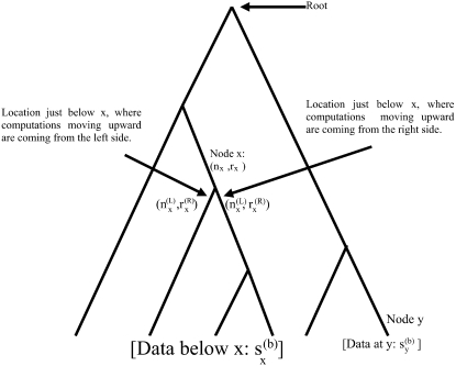
We discuss the pruning algorithm by reference to Figure 1. In Figure 1, the lower a location is in the tree, the more recent it is.

Figure 1.—

Structure of an evolutionary tree.

At this point, we introduce our notation for the different random variables used for this article (Table 1 and Figure 1). The random variables of primary interest are n_x, the number of lineages at node x, and r_x, the allele count (of n_x lineages) at node x. We considered also , the total number of haploid individuals sampled at or below node x, and , all the allele-count data at or below node x. These are required as we need to compute the probability of the data observed at or below a particular time point in the tree, conditioned on the allelic configuration at that time point. Next we use the term “a location just below a node, in the branch coming from the left (or the right) side of node x,” to mean a time-point x′ at the left branch (or the right branch), such that the time period between x and x′ is infinitesimally small (and, therefore, no coalescent event has taken place in that period).

TABLE 1.

Notation (see also Figure 1)

nx	No. of lineages at node x: nx ≥ 1
rx	Allele count (the count of “1” alleles) of nx lineages at node x: 0 ≤ rx ≤ nx
	All the data at or below node x
	All the data that are not at or below node x
	Total no. of haploids sampled at or below node
	Total no. of haploids sampled that are not at or below node x
	No. of lineages just below node x, in the branch coming from the left side of
	Allele count (of lineages) just below node x, in the branch coming from the left side of
	All the data at or below the branch coming from the left side of node x
	All the data that are not at or below the branch coming from the left side of node x
	Total no. of haploids sampled at or below the branch coming from the left side of node
	Total no. of haploids sampled that are not at or below the branch coming from the left side of node x
	No. of lineages just below node x, in the branch coming from the right side of
	Allele count [of lineages] just below node x, in the branch coming from the right side of
	All the data at or below the branch coming from the right side of node x
	All the data that are not at or below the branch coming from the right side of node x
	Total no. of haploids sampled at or below the branch coming from the right side of node
	Total no. of haploids sampled that are not at or below the branch coming from the right side of node x

Our pruning algorithm computes arrays of probabilities at each node of a tree. First, the arrays of the probabilities are computed at each tip from the data at that tip. Then the arrays of probabilities at a location (a node or a location just below a node) are computed on the basis of the location(s) just below that one (see Figure 1). By repeating this process, we eventually reach the root of the tree, where the likelihood is computed from the arrays of probabilities at the root.

At a location (at a node x, or just below a node x, in one of the two branches) there are two arrays of probabilities related to the number of coalescence events and the allele counts among the partially coalesced lineages. The first array consists of the probabilities of different numbers of lineages at that location. The probabilities are computed from the lengths of the branches between that location and the present. The second array consists of the conditional probability of the data observed at or below that location, conditional on the possible numbers of lineages in that location and the possible allele counts at those lineages. To be specific, the first array at a node x is given by

so that

The second array at a node x is two dimensional and is given by

so that

Note that the probabilities in the components of A(x) and B(x) are computed conditional on the topology, the branch lengths, and the sample sizes in the tips below node x. However, for notational simplicity we do not explicitly write them as functions of these. At a point just below and coming from the left side of node x, the first array is given by

so that

and the second array is given by

so that

A^(R)(x) and B^(R)(x) are similarly defined for a point just below and coming from the right side of node x. Note that the probabilities in the components of A^(L)(x), B^(L)(x), A^(R)(x), and B^(R)(x) are computed conditional on the topology, the branch lengths, and the sample sizes in the tips below node x. As in the cases of A(x) and B(x), for notational simplicity we do not explicitly write them as functions of these.

At a tip x the arrays of probabilities can be obtained using the fact that

and that

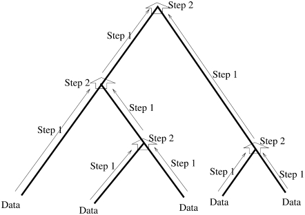
where s_x is the allele count observed at the tip x, in a sample of m_x haploids. Starting from the tips, the arrays of probabilities from the tips upward are computed recursively using two different steps. These steps are shown in Figure 2. Step 1 computes the arrays of probabilities at a location just below the top of a branch from those at the bottom node of the branch. Step 2 combines the two sets of arrays from just below a node (from the right and from the left), to obtain the arrays of probabilities at that node. The arrays at the root are computed by a final use of step 2. Then we compute the likelihood from the arrays at the root at all loci. In many standard pruning algorithms probabilities of the observations seen at or below a point on the tree are computed conditional on each of the different possible true states at that point (see, for example, Elston and Stewart 1971). These are then updated, moving rootward. Here, the presence of the coalescent, a stochastic process that moves backward in time, leads to an unusual bidirectional conditioning.

Figure 2.—

Steps of the pruning algorithm.

Step 1:

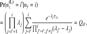
Consider a branch with bottom node y and top node z. Step 1 computes the arrays of probabilities at the location in that branch just below z from those at y. Without loss of generality, let us assume that this branch comes to z from the left side. Thus, it suffices to have a method for computing A^(L)(z) and B^(L)(z) from A(y), B(y) and from the branch length. We use equations involving two different quantities to compute the arrays of probabilities in an upward location of the tree from the arrays of probabilities at some given location(s) of the tree. One is , computed from the branch length τ_jk. This is given by Takahata and Nei (1985) as

(2)

where . The second equation is for

given by Nielsen et al. (1998) as

(3)

where β(., .) is the beta function, defined as

which equals if both u and w are positive integers. Interestingly, these two equations have probability flowing in opposite directions. This makes it difficult to obtain a straightforward transition probability. So we split the transition into two stages. At the first stage we compute A^(L)(z). The components of A^(L)(z) are computed as

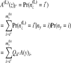(4)

using Equation 2 above. Then at the second stage we compute B^(L)(z). Bayes' theorem is used to reverse the direction of conditioning and compute the probabilities , and then these quantities are used to compute the components of B^(L)(z):

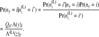(Note that is independent of the sample sizes, given n_y. Thus, Q_ii′ is free from the sample sizes at the tips.) We then obtain the components of B^(L)(z) as

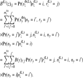(5)

Step 2:

Step 2 is analogous to step 1. Step 2 combines the two sets of arrays {A^(L)(x), B^(L)(x)} and {A^(R)(x), B^(R)(x)} just below node x, to obtain the arrays {A(x), B(x)} at node x. We make use of equations to compute two different quantities to make the transition at step 2. One is for . This is an indicator function for whether (. The other is for , which is simply the hypergeometric probability

(6)

(with i = i′ + i″ and j = j′ + j″). As in step 1, these two equations have the conditioning of the probability flowing in opposite directions. Again we split the computation into two stages. At the first stage A(x) is computed. We compute A(x) as

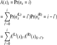Then at the second stage B(x) is computed. Bayes' theorem is used to reverse the direction of conditioning and compute the probabilities , and then these quantities are used to compute the components of B(x):

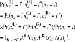We can then get the components of B(x) as

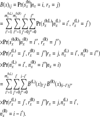(7)

These equations are analogous to the corresponding Equation 5 in step 1, but are more complicated as the arrays of probabilities from the two branches are being combined. Equation 7 uses the fact that ) and that and are independent of each other given , , , and .

Likelihood from the arrays at the root:

For convenience, let us denote the root as node 0. At the root we have arrays given by

Using these we can compute the joint likelihood of and the ancestral allele frequency p as

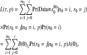Here Pr(r₀ = j | n₀ = i, p) is the binomial probability,

We assume that p has a beta(θ, θ) distribution, where the density of beta(z₁, z₂) is given by

The quantity θ is 4N_eμ, where the quantities N_e and μ are the effective population size and the mutation rate, respectively, for the common ancestral population of the populations under consideration. This gives us the marginal likelihood of as

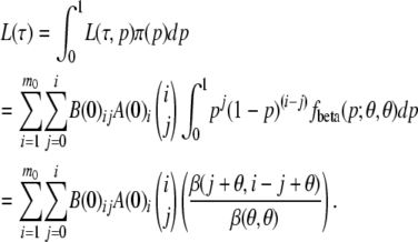The choice of this beta distribution comes from the fact that the stationary distribution of allele frequency over loci has this distribution if the population has had the same value of θ for a considerable time (Wright 1931). However, this choice is not binding. We would get a similar closed-form expression for any other beta distribution. Even for an arbitrary π we might be able to compute this likelihood numerically. This approach gives us the likelihood for a given tree with specified branch lengths. There remains the issue of efficiently maximizing the likelihood over branch lengths.

MAXIMIZING THE LIKELIHOOD OVER BRANCH LENGTHS

Due to the multidimensional parameter space we did not use any derivative-based methods (such as the Newton–Raphson method) to maximize the likelihood over branch lengths for a given topology.

This maximization strategy involves comparing different branch lengths of a particular branch of otherwise identical trees. The most efficient way of maximizing the likelihood over values of a single branch length is to implement computation of upward and downward views (Felsenstein 1981, 2004).

The upward and the downward views:

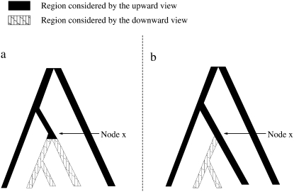
This mechanism works by storing two sets of probabilities for each locus at each node and at the locations just below each nontip node. The two sets, the upward view and the downward view for a particular locus, consist of components of likelihood that are the probabilities for the parts of the tree above and below that node (or location), respectively, at that locus. (We provide the mathematical definitions of the upward and the downward views later in this section.) Figure 3a indicates, for an example, the regions that are covered by the upward and downward views at a node; Figure 3b indicates the regions that are covered by the upward and downward views at a location just below the node on the branch going to the left side.

Figure 3.—

The regions of a tree where the arrays of probabilities affect the upward and downward views, for views at node x and for views immediately below and to the left of node x.

Suppose that we have the likelihood for one set of branch lengths and want to change the length of a branch and recompute the likelihood. Let the top and the bottom nodes of the branch be x and y, respectively. The change will affect the downward views of the nodes that are in the path from x to the root (including x and the root) and the upward views of y and the nodes below y. Using the views, the likelihood can be computed from the downward views at all loci at the bottom node of the branch, the updated length of the branch, and the upward views at all loci at the location just below the top node of the branch. The likelihood for multiple loci is computed as the product of the single-locus likelihoods.

For a locus, the downward views at a node x and at the two locations just below the node are B(x), B^(L)(x), and B^(R)(x), respectively. The upward view at node x is the array C(x). This array consists of the probabilities of allele counts at node x given the data observed at the tips that are not at or below x. These probabilities are conditioned on different possible numbers of lineages n_x at x. Thus we have the triangular array C(x) whose ij element is

with i taking values from 1 to and j taking values from 0 to i. By we have designated all the data that are not at or below node x. The upward views at the locations just below the node, at the branches coming from the left side and coming from the right side, are two arrays of probabilities C^(L)(x) and C^(R)(x). The array C^(L)(x) is the probabilities of allele counts just below node x on the branch coming from the left side of x. These probabilities are conditioned on different numbers of lineages at that location. The array C^(R)(x) is similar.

Thus we have a triangular array whose ij element is

with i taking values from 1 to and j taking values from 0 to i. As before, and denote all data that are not at or below the branch coming from the left side and the right side of node x, respectively. Also as before consider a branch with bottom node y and top node z. Without loss of generality, let us assume that this branch comes to z from the left side.

The arrays A^(L)(z)_i and B^(L)(z)_ij can be recomputed with the new branch length and the old A(y)_i and B(y)_ij as in Equations 4 and 5, respectively. For each locus, the likelihood can be recomputed after changing the length of the branch that joins y (at its bottom node) and z (at its top) coming from the left side of z, as

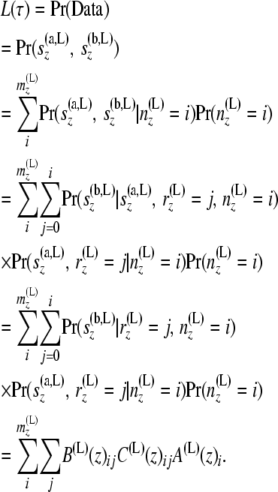The above calculation uses the fact that and are independent of each other. The likelihood for the multiple-locus data can then be recomputed as the product of the single-locus likelihoods.

If we have the downward views in a completely specified tree, then the upward views can be computed recursively starting from the root and going downward to the tips. The array C(0), the upward view at the root, is computed as

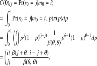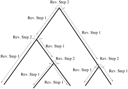
for each locus. Then, for each locus, applying a recursive formula to compute the upward views at a location from the upward and downward views just above that location, we show how we can obtain the upward views for each locus and for all the locations on the tree. (See Figure 4.)

Figure 4.—

Flow of the computation using the two reverse steps to update downward views.

The recursive formula has two parts, as was the case for the recursive formula in the section, a pruning algorithm. One part computes the upward view at the bottom of a branch from the view at the location just below the top of the branch. We call this computational step reverse step 1. The other part of the formula computes the upward view at a location just below a node from the upward views at the node and the downward view for the other branch that is just below the node. We call this computational step reverse step 2.

Reverse step 1:

In this section, we describe the workings of reverse step 1. Consider a branch with bottom node y and top node z. Assume that this branch comes to z from the left side. Let us recall that reverse step 1 computes C(y) from C^(L)(z) and the length of the branch,

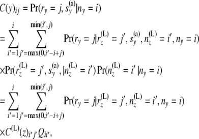(8)

where the bounds on i′ and j′ come from the following relations:

Combining (3) and (8), we have the required method for computing C(y).

Reverse step 2:

Consider a node x. Just below a node x in the branch coming from the left side, reverse step 2 computes C^(L)(x) from C(x), A^(R)(x), and B^(R)(x). Here we give formula for the computation of C^(L)(x):

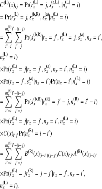(9)

where the bounds on i′ and j′ come from the following relations:

Combining (6) and (9), we have the formula for C^(L)(x). The computation of C^(R)(x) is analogous.

Maximization:

We maximize the likelihood with respect to the branch lengths for each θ in a grid of values of θ. For each value of θ, we maximize the likelihood with respect to one branch length and do this successively for each branch in the tree. For each branch we carry out a simple line search over values separated by a constant small spacing. We repeat the process, continuing until none of the branches changes in a pass through the tree. After we have maximized the likelihood for the length of a branch, if the new length is different from its previous length, we recompute all views that are affected by that change of length. Once the maximization is done for each value of θ, we compare those maximum values and pick the overall maximum.

As we are searching over a grid of fixed spacing, the maximization takes a finite number of iterations. We have no proof that this process does not yield a local maximum within a topology and that another maximum with a larger likelihood does not exist. However, we have not come across any data set where we have found two separate maxima within a topology.

This process maximizes the likelihood over branch lengths for a specified tree topology. The search for the maximum-likelihood tree involves either consideration of all possible tree topologies or heuristic searches that consider only neighboring tree topologies. For trees of moderate to large size, exhaustive consideration of all topologies is not possible. The issues and strategies involved are the same as with other phylogeny inference problems. They are not described here. Common strategies are described by Felsenstein (2004, Chaps. 4 and 5).

SIMULATION STUDIES

To test the performance of our method, we carried out two simulation studies, one with four populations (repeated 10 times) and one with seven populations. A molecular clock is not assumed in any of these studies.

To simulate a data set from a completely specified tree, we start with simulating L (number of loci) beta(θ, θ) variables: . An array of N (population size) Bernoulli(p_l) variables are generated for each . Then according to the structure of the tree, the population is divided into two groups at each node and made to evolve according to a continuous-time Moran model at each branch (by having events that consist of selecting an individual to replace another individual, independently for each locus). At each branch the population is made to evolve the exact amount of time so that the scaled time passed at that branch agrees with the length of the corresponding branch of the tree. When the populations reach at the tip of the tree, we take a sample of n individuals from each population; the data consist of the counts of 1 alleles at the L loci of all present-day populations.

In the first study the data consist of allele counts in 50 haploids from each population for 50 independent SNP loci. The data are simulated as described in the previous paragraph from a symmetric tree where the length of each branch is 0.02 and the value of θ is 0.05. Then the maximum-likelihood estimate (MLE) tree is estimated using our pruning algorithm. The same exercise is repeated 10 times, each time simulating the data independently with the same parameters. Each time the true tree was estimated by our method. The estimated bias of the branch lengths is close to 0.005 for each branch.

In the second study, we tested our pruning algorithm in a tree with seven populations; the data consist of allele counts in eight haploids from each population for 500 independent SNP loci.

Note that there are >10,000 possible topologies for a seven-population tree. We have computed only the likelihood of the true topology and the other topologies that are nearest neighbors to the true topology.

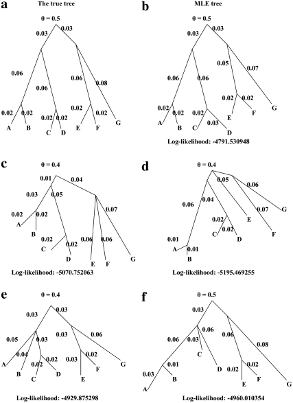
The true tree for the second study is given in Figure 5a. Among the topologies considered, the likelihood is highest for the true tree topology. The likelihood, the MLE branch lengths, and for five of the topologies are given in Figure 5, b–f. In Figure 5b, the estimated branch lengths are close to the true ones.

Figure 5.—

Results from the simulation study with seven populations.

In all cases that have misspecified topologies, the internal branches collapse to make the topology as close as to the topology of Figure 5a as possible. For example, when the branch adjacent to “G” of Figure 5b is reattached at the branch that is at the immediate right of the root, the tree of Figure 5c is the maximum-likelihood tree for the resulting topology. The internal branch created between the top of the branch adjacent to G and the meeting point of “E” and “F” collapses. (We do not have any proof that this will always be true; it is quite possible that for some data sets there may be local maxima of the likelihood for nonzero branch lengths within two or more tree topologies.)

Thus we have demonstrated that the correct topology can be estimated using our method. We saw no sign of systematic bias in the tree topology of branch lengths.

INFORMATION ABOUT THE ROOT

As mentioned in the Introduction, it is possible to estimate the root of the tree owing to the nonreversibility of the model. Here we investigate how much information a single locus provides for the estimation of the location of the root.

For simplicity we investigate the information on the location of the root in a tree with two populations. There is only one possible topology for a tree of two populations. The branch lengths determine the location of the root. As the branch lengths are time scaled by effective population sizes, the ratio of the lengths of the branches is determined by the (unknown) ratio of the effective population sizes of the branches. So, the length of each branch can be treated as a free parameter.

A tree of two populations can be completely characterized by the total length of the two branches and the location of the root. To isolate the information about the root from the information about the total length of the two branches, we assume that we are aware of the total length (τ_t = τ₁ + τ₂) of the two branches, but that the lengths (τ₁ and τ₂) of the individual branches are unknown. In other words, we assume that we do not know the location of the root in an otherwise completely specified tree with two populations. The information about the root is obtained as

(10)

where L(., .) denotes the likelihood of a tree with two tips with the two branch lengths as the two arguments. The derivative of the likelihood in (10) is computed theoretically for all possible sets of allele counts. Then the expectation of the squared derivative of the likelihood is computed numerically. The likelihood is a weighted average of the squared derivative over all possible data outcomes, weighted by the probability of each data outcome.

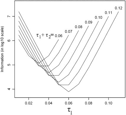
Figure 6 plots the log ₁₀ of the information about the root for different branch lengths in a tree with two tips. In each case, the information is for samples of size 10 from each tip. Figure 6 shows that the information is at a minimum at . If τ₁ ≠ τ₂, one population (Pop. 1) will be expected to have more extreme allele counts than the other (Pop. 2). Having more extreme allele counts indicates that Pop. 1 has the smaller population size of the two. Having a smaller population size indicates that the length of the branch connected to Pop. 1 is bigger than that of Pop. 2. In other words, the root is closer to Pop. 2 than to Pop. 1. As demonstrated in Figure 6, the log₁₀ of the information about the root ranges between 3 and 8 from the cases that we analyzed here. This suggests that the standard error of estimation of the root is at most of order 10⁻¹.

Figure 6.—

Information about the root from samples of (haploid) size 10 from each tip in a tree with two tips.

IMPLEMENTING AN ASCERTAINMENT CORRECTION

We can characterize the process of choice of SNPs by considering which loci will fail to be ascertained, as follows. If the observation from a locus falls into a predefined rejection set, then that locus will be excluded from study. As a simple example, let us consider a sample of diallelic SNP loci. If we want to exclude those loci that have only one allele type in a sample of haploid size m, our rejection set would be {0, m}. Table 2 shows examples of several possible ascertainment methods in one or more populations.

TABLE 2.

Ascertainment schemes and their associated rejection sets

No. of populations	Ascertainment scheme: select the locus only if:	Based on previous or current sample	Rejection set in sample(s) of (haploid) size mi from the ith population
1	Two observed alleles	Current	R = {0, m1}
1	At least two copies of the minor allele in the sample	Current	R = {0, 1, m1 − 1, m1}
3	Does not have same allele fixed, in samples from all three populations	Current	R = {(0, 0, 0), (m1, m2, m3)}
3	Each allele is observed to have at least two copies in a sample from at least one population	Current
3	Each minor allele is observed to have at least two copies in a sample from at least one population	Previous

Ascertainment based on the current sample:

Ascertainment is sometimes based on the observations in the sample under study [for example, in The SNP Consortium study (Thorisson and Stein 2003)]. In such cases, we implement an ascertainment bias correction as follows.

Let the data be

from the P populations under study. Let the rejection set be R. Then, the ascertainment-corrected likelihood for the branch length vector is given by

Here, is the same as the uncorrected likelihood. For the denominator, we need a mechanism of computing the collective probability of a set of possible observations, rather than an individual observation. One way of doing this is to compute the probability of all the individual members of the set, and sum up. We will describe a more efficient computational method than this in an upcoming publication (A. RoyChoudhury and E. A. Thompson, unpublished data).

Ascertainment based on a previous sample:

In some studies, ascertainment is done on the basis of data from a panel of SNPs (see, for example, Clark et al. 2005). To correct the bias induced by such ascertainments, we implement the following procedure.

Let us denote the data from the preliminary sample as

and the rejection set in the preliminary sample as R^(v). Then, if D^(v) is available for current analysis, the ascertainment-corrected likelihood for the branch length vector is given by

Here, is the uncorrected likelihood for the collection of D and D^(v). The denominator requires a method for computing the probability of a collective set of possible observations. An efficient way of doing this will be demonstrated in an upcoming publication by A. RoyChoudhury and E. A. Thompson (unpublished data).

DISCUSSION

From the simulation studies, it is apparent that our method performs well. The branch length estimates were found to have a low bias. We must note that the first study is based on 50 loci only. In practice, there are thousands of independent SNP loci available in humans. Conditional on the validity of the model, this large number of loci will give us much more accurate estimation of branch lengths using genomewide data.

The work in this article is an improvement on existing methods of exact-likelihood computation of a population tree using a coalescent model. It adds a manageable structure to the computation, resulting in increased tractability. Further, this method is free from use of any Monte Carlo technique and, as a result, can make a precise estimate without an indefinitely long run.

The difference in log-likelihood between competing topologies suggests that the data provide a wealth of information. We believe that this methodology will prove useful in analyzing data on polymorphisms across subspecies and populations. In theory, this method of pruning is applicable to data from loci with any number of alleles. However, the computational load of the pruning algorithm applied to a multiallelic loci could be very large. As we have to compute the probability of data conditional on all possible configurations of all the alleles at the root, the complexity will be of order o(m^κ), where κ is the total number of alleles and m is the total number of samples.

Although this is a significant improvement in computing the likelihood of a fully specified tree, the number of possible topologies makes maximum-likelihood estimation a daunting task for larger trees (>10 populations). With other kinds of data the problem of searching among tree topologies is also difficult, with some methods provably NP hard (Foulds and Graham 1982; Graham and Foulds 1982).

The maximization is done as a line search over a fixed grid. We did not use a more sophisticated method for two reasons. The first reason is that some of the more sophisticated methods are not designed for optimizing multimodal functions. It is possible that our likelihood function is multimodal as the lengths of different branch may have similar effects on likelihood. Therefore we stick to grid search. The second reason is that grid search makes the computing simpler.

We have written a software based on our method. Using this software, the likelihood for the first study (four populations) took ∼27 sec per locus to compute in a computer with 3 GHz CPU. For the second study (seven populations) it took <1 sec per locus in the same computer. The computation time can be drastically improved by efficient coding. We plan to recode parts of the software to make it more time efficient and make it available online.

References

- Cavalli-Sforza, L. L., and A. W. F. Edwards, 1967. Phylogenetic analysis. Models and estimation procedures. Am. J. Hum. Genet. 19 233–257. [PMC free article] [PubMed] [Google Scholar]
- Clark, A. G., M. J. Hubisz, C. D. Bustamante, S. H. Williamson and R. Nielsen, 2005. Ascertainment bias in studies of human genome-wide polymorphism. Genome Res. 15 1496–1502. [DOI] [PMC free article] [PubMed] [Google Scholar]
- Edwards, A. W. F., and L. L. Cavalli-Sforza, 1964. Reconstruction of evolutionary trees in phenetic and phylogenetic classifications. Syst. Assoc. Publ. 6 67–76. [Google Scholar]
- Elston, R. C., and J. Stewart, 1971. A general model for the analysis of pedigree data. Hum. Hered. 21 523–542. [DOI] [PubMed] [Google Scholar]
- Felsenstein, J., 1968. Statistical Inference and the Estimation of Phylogenies. Ph.D. Thesis, University of Chicago, Chicago.
- Felsenstein, J., 1973. a Maximum likelihood and minimum-steps methods for estimating evolutionary trees from data on discrete characters. Syst. Zool. 22 240–249. [Google Scholar]
- Felsenstein, J., 1973. b Maximum-likelihood estimation of evolutionary trees from continuous characters. Am. J. Hum. Genet. 25 471–492. [PMC free article] [PubMed] [Google Scholar]
- Felsenstein, J., 1981. Evolutionary trees from DNA sequences: a maximum likelihood approach. J. Mol. Evol. 17 368–376. [DOI] [PubMed] [Google Scholar]
- Felsenstein, J., 2004. Inferring Phylogenies. Sinauer Associates, Sunderland, MA.
- Foulds, L. R., and R. L. Graham, 1982. The Steiner problem in phylogeny is np-complete. Adv. Appl. Math. 3 43–49. [Google Scholar]
- Graham, R. L., and L. R. Foulds, 1982. Unlikelihood that minimum phylogenies for a realistic biological study can be constructed in reasonable computational time. Math. Biosci. 60 133–142. [Google Scholar]
- Heuch, I., and F. M. H. Li, 1972. PEDIG—a computer program for calculation of genotype probabilities, using phenotypic information. Clin. Genet. 3 501–504. [DOI] [PubMed] [Google Scholar]
- Hilden, J., 1970. GENEX—an algebraic approach to pedigree probability calculus. Clin. Genet. 1 319–348. [Google Scholar]
- Moran, P. A. P., 1962. The Statistical Processes of Evolutionary Theory. Clarendon Press, Oxford.
- Nielsen, R., and M. Slatkin, 2000. Likelihood analysis of ongoing gene flow and historical association. Evolution 54 44–50. [DOI] [PubMed] [Google Scholar]
- Nielsen, R., J. L. Mountain, J. P. Huelsenbeck and M. Slatkin, 1998. Maximum likelihood estimation of population divergence times and population phylogeny in models without mutation. Evolution 52 669–677. [DOI] [PubMed] [Google Scholar]
- Takahata, N., and M. Nei, 1985. Gene genealogy and variance of interpopulational nucleotide differences. Genetics 110 325–344. [DOI] [PMC free article] [PubMed] [Google Scholar]
- Thompson, E. A., 1975. Human Evolutionary Trees. Cambridge University Press, Cambridge, UK.
- Thorisson, G. A., and L. D. Stein, 2003. The SNP Consortium website: past, present and future. Nucleic Acids Res. 31 124–127. [DOI] [PMC free article] [PubMed] [Google Scholar]
- Wright, S., 1931. Evolution in Mendelian populations. Genetics 16 97–159. [DOI] [PMC free article] [PubMed] [Google Scholar]