Performance of breast ultrasound computer-aided diagnosis: Dependence on image selection

Abstract

Rationale and Objectives

The automated classification of sonographic breast lesions is generally accomplished by extracting and quantifying various features from the lesions. The selection of images to be analyzed, however, is usually left to the radiologist. Here we present an analysis of the effect that image selection can have on the performance of a breast ultrasound computer-aided diagnosis system.

Materials and Methods

A database of 344 different sonographic lesions was analyzed for this study (219 cysts/benign processes, 125 malignant lesions). The database was collected in an IRB-approved, HIPAA-compliant manner. Three different image selection protocols were used in the automated classification of each lesion: all images, first image only, and randomly selected images. After image selection, two different protocols were used to classify the lesions: A) the average feature values were input to the classifier, or B) the classifier outputs were averaged together. Both protocols generated an estimated probability of malignancy. Round-robin analysis was performed using a Bayesian neural network-based classifier. Receiver operating characteristic analysis was used to evaluate the performance of each protocol. Significance testing of the performance differences was performed via 95% confidence intervals and non-inferiority tests.

Results

The differences in the area under the ROC curves were never more than 0.02 for the primary protocols. Non-inferiority was demonstrated between these protocols with respect to standard input techniques (all images selected and feature averaging).

Conclusion

We have proven that our automated lesion classification scheme is robust and can perform well when subjected to variations in user input.

1. INTRODUCTION

Breast cancer continues to be the most common form of cancer and the second most common cause of death from cancer among women in the United States [1]. While routine mammography is currently the only screening method recommended for the general public [2], there is still considerable research being done to augment the breast cancer detection and diagnosis process. The utility of ultrasound, for example, to evaluate and diagnose lesions and abnormalities within the breast has increased dramatically over the past decade [3-6]. Previous studies have shown breast ultrasound to have an accuracy of 96%-100% in the diagnosis of cysts [7] and its use in differentiating between different types of solid lesions (i.e., benign vs. malignant) is becoming more prevalent [3-6, 8]. This increased interest in ultrasound as a diagnostic tool for breast cancer has led to, among other things, rapid developments in the application of computer-aided diagnosis (CADx) to breast sonography [9].

The automated classification of sonographic breast lesions is generally accomplished by extracting and quantifying various features from the lesions. Features such as margin shape, margin sharpness, lesion texture, and posterior acoustic behavior have been shown to be particularly useful in computerized classification schemes [10] and CADx systems based on these features have been shown to perform the benign vs. malignant classification task well [11, 12]. Such systems are still subject to several different kinds of user-induced variability, however. The choice of images to be analyzed, for example, is generally left to the user of the system. As a result, the manner in which a particular lesion is input into the system may vary between different users (i.e., radiologists). This variability may have the potential to impact the output, and thus the performance, of the classifier. Here we will present an analysis of the effect that image selection can have on the performance of a sonographic breast lesion CADx system.

2. MATERIALS AND METHODS

2.1. Image Database

A database consisting of 344 different lesions was retrospectively collected and analyzed for this study. The original breast ultrasound exams were performed at a single facility using an HDI 5000 ultrasound scanner with an HDI L12-5 scanhead (Philips Medical Systems, Bothell, WA). Each exam was performed using the same clinical imaging protocol established at the imaging site. Informed consent was obtained from patients during clinical imaging. No case selection was performed; the only requirement was that each sonographically-identified lesion had to be depicted on at least two different images. The database was collected under an Institutional Review Board-approved protocol. All applicable HIPAA regulations were observed during the collection, maintenance, and use of the database.

The database contained images of 116 cysts, 103 benign processes, and 125 malignant lesions (Table 1). Each lesion was considered an independent event (this is not considered to be an issue as we are investigating a classification task, not a detection task). Some patients presented with multiple sonographic findings. The number of images per lesion (i.e., the number of images available of a single physical lesion) varied from 2 to 20 (Figure 1). All of the malignant lesion pathologies were verified via tissue biopsy. The pathologies of the benign and cystic lesions were either verified via tissue biopsy or were felt to be so benign in nature during the original clinical examination that no further intervention was recommended. Although a radiologic interpretation would often be the final clinical workup for some cysts and benign lesions, this was not felt to be an issue as we are interested in the agreement of our algorithm with the diagnostic decision that would occur clinically. A single breast radiologist, with over 17 years of experience and certified according to the Mammography Quality Standards Act, reviewed all of the lesions in the database. The radiologist indicated seed points within all the imaged lesions. These points were then used to perform automatic segmentation of the lesions using an average radial derivative-based method [13]. It is important to note that in this study we were not investigating lesion detection methods or the accuracy of the segmentation algorithm, only the variability in the classification algorithm from different inputs once a lesion is identified. In addition, it is unlikely that the selection of different seedpoints would have an effect on our system; for a brief analysis of the potential impact that the selection of different seedpoints might have, please see Appendix 1.

Table 1.

Composition of the sonographic database.

Pathology	Biopsied?	# of patients	# of images	# of physical lesions
Cyst	Yes	48	189	62
Cyst	No	36	120	54
Benign Solid/Tumor	Yes	63	208	68
Benign Solid/Tumor	No	15	48	18
Benign Fibrocystic	Yes	15	58	17
Malignant	Yes	104	444	125
TOTALS		281	1067	344

Figure 1.

The distribution of the number of images available per lesion.

2.2 Image Selection Protocols

Three different image selection protocols were used in the automated classification of each lesion. In the first protocol, all of the images available for a particular lesion were used in the analysis (“all images”). In the second protocol, only the features from the first image of each lesion were used in the analysis (“first image only”). The “first” image of each lesion was determined by looking at the chronological order in which the images of the lesion were saved to the clinical PACS server. In the third protocol, a random set of images from each lesion was selected and used in the analysis (“random images”). Both the number of images selected and the individual images selected were randomized for each lesion in this protocol. These three different image, or “view,” selection protocols were meant to mimic the variability in user (radiologist) input (Figure 2): the “all images” protocol was meant to mimic a radiologist who identifies a lesion of interest on every available image for input to an automated classifier, the “random images” protocol was meant to mimic a radiologist who arbitrarily identifies a lesion on a few images for input, and the “first image only” protocol was meant to mimic a radiologist who only identifies a lesion on the first available image for input. Our experience with observer studies suggests that these available methods of input available for our automated classifier. For the sake of completeness, two additional view selection protocols were also performed: “single random image,” in which a single image of each lesion was randomly selected for analysis, and “second image only,” in which only the second image of each lesion was selected for analysis. These protocols were meant to directly augment the “first image only” protocol, as all three involve the rather arbitrary selection of a single image.

Figure 2.

Four different images depicting the same physical lesion. In the “all images” view selection protocol, features from all four of the images are extracted and used in analysis (indicated by a solid outline). In the “first image only” view selection protocol, only features from the first image are used in analysis (indicated by the dashed-dotted outline). In the “random images” view selection protocol, only features from a randomly selected group of images are used in analysis (indicated by a dashed outline); in this example, two of the four images were randomly selected via this protocol.

2.3 Lesion Classification Protocols

Four sonographic features were extracted from every image of each lesion in the database: lesion shape, margin sharpness, posterior acoustic shadowing, and lesion texture. These features are known to be useful in clinical practice during a diagnostic evaluation [3, 14]. A rigorous mathematical description of these features can be found elsewhere [10, 13].

After view selection, two different protocols were used to classify the lesions. In the first protocol (protocol “A”), the average value of each lesion feature is calculated using all of the images selected for a particular lesion (Figure 3). These average feature values are then input to a Bayesian neural network-based (BNN) classifier with 5 hidden units [15] and an estimated probability of malignancy is generated. In the second protocol (protocol “B”), lesion features from each of the selected images are input to the classifier separately and then these classifier outputs are averaged together, again providing an estimated probability of malignancy (Figure 3). These two classification protocols were chosen to test the robustness of some common methods of data input for an automated classification scheme. A third protocol in which neither lesion feature averaging nor classifier output averaging was performed is provided as a reference comparison (protocol “C”).

Figure 3.

A flowchart depicting the two main protocols used to evaluate our BNN classifier. In protocol A, features from multiple images of the same physical lesion are extracted and averaged together before they are input into the classifier. In protocol B, features from multiple images of the same physical lesion are input into the classifier directly, and then the classifier outputs from each of these images are averaged together.

2.4 Performance Assessment and Statistical Analysis

Round-robin analysis (also called the “leave-one-out” method) was performed using our BNN classifier. This analysis method trains the classifier using every lesion in the database except for one; the lesion left out of the training set is used to test the classifier. This process is repeated by leaving a different lesion out of the training set each time until every lesion has been used to test the classifier. This ensures that images from the same lesion are never used in both the training and testing sets simultaneously. It should be noted that there is a difference in classifier training between protocols A and B; the classifier used in the round-robin testing of protocol A is trained using the average features of all the lesions in the database (minus the test lesion) while the classifier used in the round-robin testing of protocol B is trained using all of the features. This is done to ensure that the classifier is trained under the same conditions that it will be tested under. With this model we are mostly interested in tester variability (as opposed to trainer variability) because we wanted to assess the performance uncertainty of a well-defined neural network trainer. Also note that the training method for each classification protocol remained constant for all related view selection protocols. In protocol B, for example, training was always conducted using features from all of the images in the training set and only the test set was varied according to the view selection protocols. As such, there would be no difference between the training procedures for “protocol B all images,” “protocol B random images,” and “protocol B first image only.” The procedure for protocol A was similar.

Receiver operating characteristic (ROC) curves [16, 17] were generated for each test using the proproc software package [18, 19]. ROC analysis allows one to compare the possible tradeoffs between the true positive fraction (TPF or sensitivity), or the probability that an actually positive case is classified as positive, and the false positive fraction (FPF or 1-specificity), or the probability that an actually negative case is classified as positive, of a diagnostic system or tool. The operational relationship between the TPF and FPF defines the ROC curve and describes the performance of a system in a way that allows for meaningful comparison to other systems [20]. All of the different combinations of view selection and classification protocols were evaluated in this manner. In our database, malignant lesions were considered positive while cysts and benign lesions were considered negative.

The performance of each different protocol combination was measured by estimating the area under the ROC curve (AUC). The proproc software package was also used to calculate the non-parametric Wilcoxon estimate of the AUC for each curve. The two-sided 95% confidence interval of each AUC was estimated using the bootstrap method described by Mossman [21] with 1000 iterations for each calculation.

Performance comparisons of the different protocols were accomplished by evaluating the differences in the AUCs (ΔAUC). Significance testing of these comparisons was accomplished via both two-sided 95% confidence intervals and non-inferiority testing. Usually, for a performance difference to be considered statistically significant its two-sided 95% confidence interval must not include zero [22]. For our purposes, however, it is not always necessary to demonstrate a statistically significant performance difference; only that there is no statistically significant decrease in performance when comparing to a reference. One-sided 95% confidence intervals were calculated for each of the comparisons that were performed when the difference between the AUCs was small (ΔAUC < 0.02). These intervals allow us to conclude with 95% certainty that the true value of the difference in AUC is higher than the lower limit of the interval [22]. The use of a one-sided confidence interval to demonstrate that the performance of one method is not worse than a reference (i.e., non-inferior) is useful for evaluating the potential near-equivalence of the two methods when a potential increase in performance is not necessary because other properties render the new method interesting (and often even a small decrease is acceptable); only the presence of a potential (sizeable compared to the task at hand) performance decrease is of concern. This type of significance testing is very common in the pharmaceutical industry, for example, when evaluating the effectiveness of a generic form of a drug against a brand-name counterpart: the intent is to demonstrate that the generic drug is capable of providing at least the same level of effectiveness as the standard, brand-name drug (i.e., that it is non-inferior) [23, 24]. Similarly, this method is often used in radiology when evaluating the effectiveness of a new, less invasive diagnostic technique against the current gold standard. In our study, non-inferiority was concluded if the lower limit of the confidence interval was larger than -0.02 (The largest ΔAUC we found between the view selection protocols when using some form of averaging was 0.02, which is fairly small and, in our opinion, too small to be of importance at this stage of development. Future developments might require a stricter definition, as might specific applications; in general, however, this difference seems to be too small to be of concern). The upper limit of the interval is inherently irrelevant, but in the case of our metric it can never exceed one; as such, the upper limit of our intervals is always one. All of the two-sided 95% confidence intervals and non-inferiority intervals are bias corrected and accelerated (BCa) and were calculated using the techniques described by Mossman [21]. Further information on the application of the Mossman methods to our data can be found in Appendix 2.

3. RESULTS

An initial examination of the output of the different classification protocols indicates that they tended to agree with each other, even when the difference in the estimated probability of malignancy for specific lesions was “large” (Figures 4 and 5). The ROC curves generated by protocol A for all three view selection protocols demonstrate that selecting all of the images available for a particular lesion yields the largest estimated AUC (0.86) when compared to the other two selection protocols (Figure 6). The same observation also holds true for the “all images” protocol with classification protocol B (AUC=0.87) (Figure 7). Protocol C (Figure 8) had the lowest overall performance (0.83) of any of the protocol combinations (Table 2). It is worth noting that the datasets used to produce the results for the “first image only” protocol of classification protocols B and C are inherently identical; as such the ROC curves for these two protocols are also identical. Analysis of the “single random image” protocol yielded an AUC of 0.84 with a 95% confidence interval of [0.788; 0.878] using protocol A and an AUC of 0.84 [0.803; 0.887] using protocol B. Analysis of the “second image only” protocol yielded an AUC of 0.81 [0.759; 0.858] using protocol A and 0.81 [0.755; 0.853] using protocol B.

Figure 4.

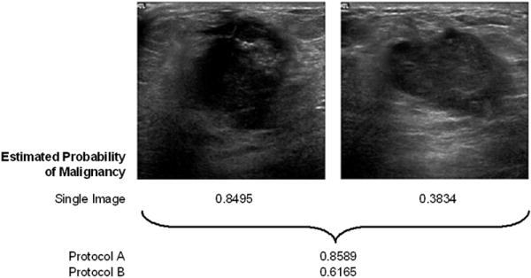
An example of a lesion with a relatively large difference in estimated probability of malignancy between the two different classification protocols. Both images depict the same physical lesion, a biopsy-proven carcinoma. The estimated probability of malignancy for each image individually is 0.8495 and 0.3834 respectively. The estimated probability of malignancy for the lesion is 0.8589 when using classification protocol A (feature averaging) and it is 0.6165 when using protocol B (classifier output averaging), demonstrating a difference of 0.24 between the two protocols. The “all images” view selection protocol was used in this example.

Figure 5.

An example of a lesion with a relatively small difference in estimated probability of malignancy between the two different classification protocols. All three images depict the same physical lesion, an aspiration-proven cyst. The estimated probability of malignancy for each image individually is 0.0791, 0.0388, and 0.0323 respectively. The estimated probability of malignancy for the lesion is 0.0434 when using classification protocol A (feature averaging) and it is 0.0501 when using protocol B (classifier output averaging), demonstrating a difference of 0.007 between the two protocols. The “all images” view selection protocol was used in this example.

Figure 6.

ROC curves resulting from the round robin testing of the different view selection protocols when using feature averaging during classification (protocol A) (N=344 for each test).

Figure 7.

ROC curves resulting from the round robin testing of the different view selection protocols when using classifier output averaging during classification (protocol B) (N=344 for each test).

Figure 8.

ROC curves resulting from the round robin testing of the different view selection protocols when no averaging is used (i.e., neither feature nor classifier output averaging) during classification (protocol C) (N=1067 for the “all images” protocol and N=517 for the “random images” protocol).

Table 2.

Results of round-robin analyses for all classification and view selection protocols given as the area under the ROC curve.

	Classification Protocol
View Protocol	A	B	C
All images	0.86 [0.813; 0.895]	0.87 [0.827; 0.905]	0.83 [0.758; 0.861]
Random images	0.85 [0.806; 0.889]	0.85 [0.810; 0.892]	0.83 [0.745; 0.870]
First image only	0.86 [0.811; 0.893]	0.86 [0.816; 0.898]	0.86 [0.816; 0.898]

Note – Data are indicated as AUC [two-sided 95% confidence interval].

Protocol A: Feature averaging

Protocol B: Classifier output averaging

Protocol C: No averaging

When comparing the performances of the different view selection protocols within each classification protocol, three comparisons produced an estimated ΔAUC of at least 0.02: protocol B “all images” vs. “random images,” protocol C “first image only” vs. “random images,” and protocol C “all images” vs. “first image only.” In the first two instances, the two-sided 95% confidence interval for the ΔAUC included zero and thus failed to show a statistically significant difference in performance. All of the remaining comparisons demonstrated non-inferiority according to the criteria previously described with the exception of the “all images” vs. “random images” protocol in classification protocol C (Table 3).

Table 3.

Differences in performance between the view selection protocols for each classification protocol.

	Classification Protocol
View Protocol Comparison	A	B	C
All images vs Random images	+0.01 [0.00; 1]†	+0.02 [0.00; 0.04]*	+0.00 [-0.02; 1]†
All images vs First image only	+0.00 [0.00; 1]†	+0.01 [0.00; 1]†	-0.04 [-0.08; -0.01]*
First image only vs Random images	+0.01 [0.00; 1]†	+0.00 [0.00; 1]†	+0.04 [0.00; 0.09]*

Note – Data are indicated as ΔAUC [confidence interval].

Protocol A: Feature averaging

Protocol B: Classifier output averaging

Protocol C: No averaging

^*Two-sided 95% confidence interval

^†Non-inferiority interval

Comparing the performances of the different classification protocols yielded statistically significant differences between protocols A and C and protocols B and C (these values are not corrected with regards to multiple comparisons issues). Comparisons of the performances of protocols B and A demonstrated non-inferiority (Table 4).

Table 4.

Differences in performance between the classification protocol for each view selection protocol.

	Classification Protocol Comparison
View Protocol	B vs. A	A vs. C	B vs. C
All images	+0.01 [0.00; 1]†	+0.04 [0.01; 0.09]*	+0.05 [0.03; 0.10]*
Random images	+0.00 [0.00; 1]†	+0.03 [0.00; 0.09]*	+0.03 [0.00; 0.09]*

Note – Data are indicated as ΔAUC [confidence interval].

Protocol A: Feature averaging

Protocol B: Classifier output averaging

Protocol C: No averaging

^*Two-sided 95% confidence interval

^†Non-inferiority interval

4. DISCUSSION

Our results demonstrated a trend of non-inferiority for nearly every view protocol comparison, indicating that no single protocol was clearly inferior to any of the other protocols. Of the comparisons that demonstrated performance differences of at least ΔAUC=0.02, two of these differences were not statistically significant (protocol B “all images” vs. “random images” and protocol C “first image only” vs. “random images”). Non-inferiority intervals for those comparisons, however, demonstrate non-inferiority: the interval of the ΔAUC for protocol B “all images” vs. “random images” is [0.00; 1] and the interval for protocol C “first image only” vs. “random images” is [0.01; 1]. The “all images” vs. “random images” protocol for classification protocol C demonstrates neither non-inferiority nor a statistically significant difference (the two-sided 95% confidence interval for this comparison is [-0.03; 0.02]). This initially suggests that there may be no difference between these two protocols when using classification protocol C, but as we will discuss later protocol C is generally not recommended in any case. Overall these results suggest that differences in user input are likely to have at most a modest effect on the performance of our automated classification scheme. This would allow the user to select images for analysis with our scheme in any manner (s)he sees fit without affecting the stability of its performance. Providing the user with this level of freedom increases the versatility of the system since its performance is relatively unaffected by a particular user’s diagnostic style, making it easier to incorporate into a clinical workflow without requiring significant increases in user training or patient workup. This is also likely to reduce observer time, all of which are likely to reduce costs.

Our results also demonstrated a trend of non-inferiority between the performances of classification protocols A and B, which suggests that the point at which averaging occurs (either feature averaging or classifier output averaging) is unlikely to have a large impact on the overall performance of the classification scheme. An inspection of the performance results of classification protocol C (Table 2) suggests that while it does not matter when averaging occurs, the act of averaging within a particular lesion is likely to have a positive impact on classifier performance. A comparison of the performance differences between the three classification protocols (Table 4) does in fact show a statistically significant increase in performance when some form of averaging is used (note that multiple comparisons are not strictly necessary here because we are looking at the trend in the whole set of comparisons —A and B vs. C— and not selecting one or two out). This is not entirely surprising as previous studies have shown that combining image information via averaging tends to be helpful in non-medical image science [25] and it yields a positive improvement in diagnostic performance in medical imaging as well [26, 27]. It is likely that averaging is able to filter out some of the noise associated with outliers that are generated during the feature extraction or lesion classification process.

It is also worth noting that the “first image only” view selection protocol performed nearly as well as the “all images” protocol for both classification protocols. This result initially seems counterintuitive as it suggests that the process of averaging information from several images of the same lesion is not any more useful than simply selecting a single image as representative of the entire lesion. Both the “single random image” and “second image only” protocols, however, performed consistently lower than the “first image only” protocol (0.84 and 0.81 vs 0.86, respectively). These lower AUCs indicate that arbitrarily selecting a single image will not provide the same level of performance that averaging the information of several images can, but the performance of the “first image only” protocol suggests that it may be possible to select a single image that provides a good representation of the lesion overall. An evaluation of the clinical imaging protocols used to perform the sonographic exams in our database confirmed this conclusion as it was noted that in clinical practice it is customary for a radiologist at our imaging site to save the “best” image of a lesion first. While the determination of the “best” image of a lesion is obviously a matter of professional interpretation and opinion, it is nonetheless useful to understand its impact in our automated classification scheme. If the clinical principles and procedures that result in the first image of a breast lesion being the “best” image can be consistently repeated, then we have demonstrated an advantage in clinical protocol that does not require image averaging. If they cannot be consistently repeated, then some form of averaging is necessary to maintain the same level of performance. As our results indicate that averaging does not have a negative effect on performance, its use would not hinder diagnostic accuracy and it would have only minimal computational and procedural impact (while it may be more time consuming for the radiologist to select the “best” image). Please note that these were very experienced radiologists who specialize in breast imaging, so it is fairly reasonable to assume that other, general radiologists would be less likely to select a meaningful “best” image.

While most of our results indicate that the view selection and classification protocols are not inferior to one another, they do not exclude that there may be a performance increase associated with one or more of our comparisons. Based on the magnitudes of our performance differences, however, any possible increase is likely to be negligible and not warrant the time and cost necessary to confirm there is improvement at this stage of development. There is certainly no large-scale improvement noted between the view selection or classification protocols.

Overall we have demonstrated that our automated sonographic breast lesion classification scheme is robust and can perform reliably when subjected to large variations in user input. This makes it a very good candidate for use as a breast ultrasound computer-aided diagnosis system. By demonstrating its performance stability we have shown its viability and efficacy as a diagnostically-useful clinical tool. It is expected that such a system would enhance the diagnosis of sonographic breast lesions by increasing radiologist accuracy, particularly at locations where an expert breast radiologist may not be present.

Appendix 1

To investigate the effect that seedpoint selection might have on the lesion segmentation process, a simulation was conducted. Lesions identified on 705 different images were outlined by a radiologist. The center-point of each outline was calculated and used as the input to the automated segmentation process [13]. Additionally, 20 different points from within each outline were selected and used to perform automated segmentation. These points were randomly selected and were constrained to lie within a mask with the same shape and center-point as the original lesion but half its size. These constraints were enacted for two reasons: first, since we are not investigating the ability of the user or the system to detect lesions, we are assuming that the lesions have already been correctly identified; and second, when training users on the operation of our system, they are instructed to place their seedpoint on the center of the lesion of interest. Our experience with observer studies has demonstrated that the choice of constraining the random points to within a “half-size lesion mask” is not unreasonable as a brief analysis of our observer data suggests that radiologists participating in our studies place seedpoints in this manner 99% (1392/1406) of the time (8 different radiologists reviewing 359 sonographic lesions; note that not all radiologists reviewed the same lesions). Once the automated segmentation has finished, the amount of overlap, O, between the lesion outlines generated with the random points, R, and the outline generated with the center-point, C, is calculated by

$$O=\frac{\mathit{Area}\left(C\cap R\right)}{\mathit{Area}\left(C\cup R\right)},$$

where O ranges from zero to one with zero representing no overlap and one representing a perfect match. The median value of the overlap was 0.924 with a 95% confidence interval of [0.922; 0.927]. The distribution of overlap values (Figure A1) demonstrates that the seedpoint selected to begin automated segmentation has only a minimal effect on the segmentation process and that overall the process is fairly consistent. Instances of extremely low overlap (O < 0.3) were often the result of random seedpoints that were as far from the center of the lesion as the constraints would allow, which is much less likely to occur if the user is instructed to place seedpoints on the center of the lesion (it is also less likely if the lesions are oddly shaped, as the lesion center becomes more “obvious” in those cases). If the random seedpoints are constrained to lie within a mask that has the same shape and center-point as the original lesion but only a quarter of its size, the median overlap improves to 0.943 [0.941; 0.945]. Again this “quarter-size lesion mask” constraint is not unreasonable as over time the user can be trained to place his/her seedpoints as close to the center of a lesion as possible with minimal effort (using our observer data from above, radiologists placed seedpoints in this manner 93% (1313/1406) of the time). When comparing the values of the sonographic features extracted from the outlines, the average difference between the center seedpoint- and random seedpoint-generated outline feature values is nearly zero for all four features (Table A1). If the random seedpoints are constrained with a quarter-size mask instead of a half-size mask, the average feature differences remain consistent; only the average difference in the RGI value decreased significantly (p-value = 0.0001). While the feature value standard deviations were not negligible, they seem to be small enough to conclude that overall the automated segmentation process is robust and can operate consistently with variations in input. However, we have also shown that it may be useful to pay more attention to seedpoint placement as the effect it might have is small but not necessarily irrelevant.

Figure A1.

Histogram depicting the distribution of overlap values between center-point-generated lesion outlines and random-point-generated lesion outlines.

Table A1.

Average difference in feature values between outlines generated using the center of the lesion and outlines generated using a random point within the lesion. Feature values have been normalized to between zero and one.

Feature Difference
Random Seedpoint Constraint	D2W		RGI		MSD		Corrl
	Mean	SD	Mean	SD	Mean	SD	Mean	SD
Quarter-size Mask	< 0.001	0.053	0.001	0.085	-0.002	0.057	0.002	0.110
Half-size Mask	< 0.001	0.060	0.005	0.098	-0.002	0.066	< 0.001	0.120

D2W: Depth-to-width ratio (shape)

RGI: Radial gradient index (shape and sharpness)

MSD: Maximum side difference (posterior acoustic behavior)

Corrl: Autocorrelation in depth direction (texture and shape)

Appendix 2

In order to validate the use of the bias-corrected and accelerated (BCa) bootstrap confidence intervals of the AUC differences [21] for our type of data, a simulation of our experimental process was conducted. A sequence of one thousand groups of coupled datasets, each representing the type of comparisons we made, was generated. Each group consisted of two datasets to represent the two protocols being compared. Each dataset consisted of a simulated test-result value for 125 “true” cases and 219 “false” cases. For the false cases, values were sampled from a normal distribution with a mean of 0 and standard deviation of 1 while the true cases from one with a mean of a/b and standard deviation of 1/b — where a and b have the same meaning as the a and b parameters of a conventional ROC curve, but were obtained from a proproc fit to one of our real datasets, following the transformations described in Metz and Pan [28] — we will call these values “x”. The cases in each coupled dataset were correlated with a correlation value similar to that of our real datasets (ρ = 0.85). We used the same correlation for positive and for negative cases as the difference in these values was generally never larger than 0.02 in our real data. Each value in the datasets was then transformed using the equations described by Metz and Pan [28] to insure that the values were samples from a “proper” binormal distribution (i.e., the variable “x” was transformed into the variable “v” following the notation used in [28]). This was done because a non-proper curve has not been observed in large scale studies. The bootstrap procedure was applied to each coupled dataset (1000 iterations per procedure) to generate a BCa confidence interval for the ΔAUC between the pair. As previously stated, the process of generating random datasets and bootstrapping to get the confidence interval for their ΔAUCs was repeated 1000 times. For the confidence intervals to be considered accurate, they need to contain zero approximately 95% of the time (indicating there is no difference in the AUCs between the datasets, which is how we built them). Overall the confidence intervals contained zero 93.8% of the time (938/1000), with 2.8% (28/1000) of the intervals being completely positive and 3.4% (34/1000) of the intervals being completely negative — this is within the estimation uncertainty for a sample of 1000 simulations, which is 1.4%, following binomial statistics. The simulation was also repeated using datasets clustered following our experimental design with similar results: the confidence interval contained zero 95.4% of the time (954/1000), with 3.1% (31/1000) of the intervals being completely positive and 1.5% (15/1000) of the intervals being completely negative. These findings demonstrate that the estimated bootstrap-BCa confidence intervals allow meaningful inference when applied to correlated and/or clustered datasets similar to ours.

References

- 1.Edwards BK, Brown ML, Wingo PA, et al. Annual report to the nation on the status of cancer, 1975-2002, featuring population-based trends in cancer treatment. J Natl Cancer Inst. 2005;97:1407–1427. doi: 10.1093/jnci/dji289. [DOI] [PubMed] [Google Scholar]
- 2.Elmore JG, Armstrong K, Lehman CD, Fletcher SW. Screening for breast cancer. JAMA. 2005;293:1245–1256. doi: 10.1001/jama.293.10.1245. [DOI] [PMC free article] [PubMed] [Google Scholar]
- 3.Fine RE, Staren ED. Updates in breast ultrasound. Surg Clin North Am. 2004;84:1001–1034. doi: 10.1016/j.suc.2004.05.004. [DOI] [PubMed] [Google Scholar]
- 4.Kolb TM. Breast US for screening, diagnosing, and staging breast cancer: Issues and controversies; RSNA Categorical Course in Diagnostic Radiology Physics: Advances in Breast Imaging – Physics, Technology, and Clinical Applications 2004. Radiologic Society of North America; Chicago, IL: 2004. pp. 247–257. [Google Scholar]
- 5.Berg WA, Gutierrez L, NessAiver MS, et al. Diagnostic accuracy of mammography, clinical examination, US, and MR imaging in preoperative assessment of breast cancer. Radiology. 2004;233:830–849. doi: 10.1148/radiol.2333031484. [DOI] [PubMed] [Google Scholar]
- 6.Berg WA, Blume JD, Cormack JB, Mendelson EB, Madsen EL. ACRIN 6666 Investigators. Lesion detection and characterization in a breast US phantom: results of the ACRIN 6666 investigators. Radiology. 2006;239:693–702. doi: 10.1148/radiol.2393051069. [DOI] [PubMed] [Google Scholar]
- 7.Jackson VP. The role of US in breast imaging. Radiology. 1990;177:305–311. doi: 10.1148/radiology.177.2.2217759. [DOI] [PubMed] [Google Scholar]
- 8.Sickles EA. Breast imaging: From 1965 to the present. Radiology. 2000;215:1–16. doi: 10.1148/radiology.215.1.r00ap151. [DOI] [PubMed] [Google Scholar]
- 9.Weinstein SP, Conant EF, Sehgal C. Technical advances in breast ultrasound imaging. Semin Ultrasound CT MRI. 2006;27:273–283. doi: 10.1053/j.sult.2006.05.002. [DOI] [PubMed] [Google Scholar]
- 10.Horsch K, Giger ML, Venta LA, Vyborny CJ. Computerized diagnosis of breast lesions on ultrasound. Med Phys. 2002;29:157–164. doi: 10.1118/1.1429239. [DOI] [PubMed] [Google Scholar]
- 11.Horsch K, Giger ML, Vyborny CJ, Venta LA. Performance of computer-aided diagnosis in the interpretation of lesions on breast sonography. Acad Radiol. 2004;11:272–280. doi: 10.1016/s1076-6332(03)00719-0. [DOI] [PubMed] [Google Scholar]
- 12.Horsch K, Giger ML, Vyborny CJ, Lan L, Mendelson EB, Hendrick RE. Classification of breast lesions with multimodality computer-aided diagnosis: observer study results on an independent clinical data set. Radiology. 2006;240:357–368. doi: 10.1148/radiol.2401050208. [DOI] [PubMed] [Google Scholar]
- 13.Horsch K, Giger ML, Venta LA, Vyborny CJ. Automatic segmentation of breast lesions on ultrasound. Med Phys. 2001;28:1652–1659. doi: 10.1118/1.1386426. [DOI] [PubMed] [Google Scholar]
- 14.Madjar H, Jellins J. The practice of breast ultrasound: Techniques, findings, differential diagnosis. 1. Stuttgart, NY: Thieme; 2000. [Google Scholar]
- 15.Kupinski MA, Edwards DC, Giger ML, Metz CE. Ideal observer approximation using Bayesian classification neural networks. IEEE Trans Med Imaging. 2001;20:886–899. doi: 10.1109/42.952727. [DOI] [PubMed] [Google Scholar]
- 16.Metz CE. Fundamental ROC analysis. In: Beutel J, Kundel HJ, Van Metter RL, editors. Handbook of medical imaging, volume 1: Physics and psychophysics. 1. Bellingham, WA: SPIE Press; 2000. pp. 751–764. [Google Scholar]
- 17.Obuchowski NA. Receiver operating characteristic curves and their use in radiology. Radiology. 2003;229:3–8. doi: 10.1148/radiol.2291010898. [DOI] [PubMed] [Google Scholar]
- 18.Pesce LL, Metz CE. [July 1, 2007];Proproc v2.2.0. Department of Radiology, University of Chicago. http://xray.bsd.uchicago.edu/krl/roc_soft.htm. Updated February 27, 2007.
- 19.Pesce LL, Metz CE. Reliable and computationally efficient maximum-likelihood estimation of “proper” binormal ROC curves. Acad Radiol. 2007;14:814–829. doi: 10.1016/j.acra.2007.03.012. [DOI] [PMC free article] [PubMed] [Google Scholar]
- 20.Pepe MS. The statistical evaluation of medical tests for classification and prediction. 1. New York, NY: Oxford University Press; 2004. [Google Scholar]
- 21.Mossman D. Resampling techniques in the analysis of non-binormal ROC data. Med Decis Making. 1995;15:358–366. doi: 10.1177/0272989X9501500406. [DOI] [PubMed] [Google Scholar]
- 22.Glantz SA. Primer of biostatistics. 6. New York, NY: McGraw-Hill; 2005. pp. 219–251. [Google Scholar]
- 23.Pocock SJ. The pros and cons of noninferiority trials. Fundam Clin Pharmacol. 2003;17:483–490. doi: 10.1046/j.1472-8206.2003.00162.x. [DOI] [PubMed] [Google Scholar]
- 24.Piaggio G, Elbourne DR, Altman DG, Pocock SJ, Evans SJW. Reporting of noninferiority and equivalence randomized trials: An extension of the CONSORT statement. JAMA. 2006;295:1152–1160. doi: 10.1001/jama.295.10.1152. [DOI] [PubMed] [Google Scholar]
- 25.Jenkins R, Burton AM. 100% accuracy in automatic face recognition. Science. 2008;319:435. doi: 10.1126/science.1149656. [DOI] [PubMed] [Google Scholar]
- 26.Huo Z, Giger ML, Vyborny CJ. Computerized analysis of multiple-mammographic views: Potential usefulness of special view mammograms in computer-aided diagnosis. IEEE Trans Med Imaging. 2001;20:1285–1292. doi: 10.1109/42.974923. [DOI] [PubMed] [Google Scholar]
- 27.Liu B, Metz CE, Jiang Y. Effect of correlation on combining diagnostic information from two images of the same patient. Med Phys. 2005;32:3329–3338. doi: 10.1118/1.2064787. [DOI] [PubMed] [Google Scholar]
- 28.Metz CE, Pan X. “Proper” binormal ROC curves: Theory and maximum-likelihood estimation. J Math Psychol. 1999;43:1–33. doi: 10.1006/jmps.1998.1218. [DOI] [PubMed] [Google Scholar]