Optimal wavelet transform for the detection of microaneurysms in retina photographs

Abstract

In this article, we propose an automatic method to detect microaneurysms in retina photographs. Microaneurysms are the most frequent and usually the first lesions to appear as a consequence of diabetic retinopathy. So, their detection is necessary for both screening the pathology and follow up (progression measurement). Automating this task, which is currently performed manually, would bring more objectivity and reproducibility. We propose to detect them by locally matching a lesion template in subbands of wavelet transformed images. To improve the method performance, we have searched for the best adapted wavelet within the lifting scheme framework. The optimization process is based on a genetic algorithm followed by Powell’s direction set descent. Results are evaluated on 120 retinal images analyzed by an expert and the optimal wavelet is compared to different conventional mother wavelets. These images are of three different modalites: there are color photographs, green filtered photographs and angiographs. Depending on the imaging modality, microaneurysms were detected with a sensitivity of respectively 89.62%, 90.24% and 93.74% and a positive predictive value of respectively 89.50%, 89.75% and 91.67%, which is better than previously published methods.

I. INTRODUCTION

Diabetic retinopathy (DR) has become a major public health issue because it is one of the main sources of blindness. In particular, epidemiological studies carried out in industrialized countries classify DR amongst the four main causes of sight problems over the whole population and the first cause of blindness before 50 years old [1][2]. Economic issues are also at stake. For example, 600 million dollars could potentially be saved every year in the United States by improving early detection of DR [3].

DR is a progressive pathology: its severity is determined by the number and the types of lesions present on the retina. As a consequence, there is a need to detect those lesions either for screening DR or for measuring its progression. Currently, lesion detection is performed manually. Automating this task would primarily be interesting in terms of objectivity and reproducibility. Moreover, if screening or follow up becomes more widely accepted, automatic segmentation will be necessary to replace physicians in the time consuming process of detection.

Microaneurysms (MAs), which are small swellings appearing on the side of tiny blood vessels, are the most frequent and often the first lesions to appear as a consequence of DR. Therefore, within this study we focused on detecting this kind of lesion. Several algorithms have been proposed to detect MAs in retina photographs. They always involve a sequence of different processing tasks. The first family of processing usually involves removing vessels for instance using mathematical morphology [4][5][6], including the top-hat transform [7]. Images are then enhanced and normalized, particularly to overcome lighting variations, by median filtering [8][6], histogram equalization [8] or retina specific treatments [9]. Different features (such as shape features or brightness) are then extracted. The use of statistical classifiers has been proposed [10][7][11][9] to detect the lesions using extracted features. In [12], preprocessed images are directly classified by a neural network (without extracting features). The two previous approaches have been combined, thus [13], [7], [9] or [14] propose hierarchical classifiers that first perform a pixel-wise classification to extract candidate lesions and then a statistical classifier was used to reject.

A matched filter is used in some studies to enhance the lesion shape using Gaussian [5][9] or special-purpose filters [12][15]. Matched filters have also been widely used on retinal images to extract blood vessels in particular [16][17][18][19], usually Gaussian filters [16][19], sometimes morphological filters [20]. In [19], a binary and a Kirsch template matched filter were also used.

In this article we introduce a new template-matching based algorithm to detect MAs. A related approach has already been proposed to detect pulmonary nodules in Helical CT Images, using a Gaussian function as template [21].

The images we study present important lighting variations and are somewhat noisy. So, template-matching cannot be efficiently performed on raw images and lesion features have to be enhanced. For this reason, we propose template-matching in the wavelet domain: in this domain, without other image processing, it is possible to solve problems caused by lighting variations or high frequency noise by choosing the working subbands. Another contribution of this article is to design a wavelet family “optimally adapted” to the problem. Several researchers have put forward methods to design a wavelet to match a specified signal in the least squares sense ([22][23]). We propose a design with a higher level of criterion: finding the wavelet that is best able to discriminate lesions from lesion-free areas. The proposed detection algorithm was evaluated on a database of multimodal retinal photographs.

The article plan is as follows. Section II-A describes our image database. Section II-B introduces and validates a model for MAs, which is required for template-matching. Section II-C presents the core of the proposed method: template-matching and how it is adapted in the wavelet domain. Section II-D discusses the choice of the wavelet filter and proposes the use of the lifting scheme. Section II-E describes our parameter selection procedure. In section III the results are presented. We end with a discussion and conclusion in section IV.

II. MATERIAL AND METHOD

A. The Database

The database contained both 914 color photographs acquired for screening purposes and 995 multimodal photographic images acquired from 52 diabetic patients for follow up (an example is given in figure 1). These photographic modalities brought complementary information about each DR lesion type. The disease severity of the above-mentioned 52 patients, according to the disease severity scale [24], is shown in table I.

Fig. 1.

Series of retina images from a patient file. Angiographs are obtained by injecting a contrast product and taking several snapshots to obtain a temporal series: (d)(e)(f).

TABLE I.

Patient disease severity distribution

disease severity	1 (no DR)	2	3	4	5	6
number of patients	4	8	16	7	8	9

These images have a definition of 1280 pixels/line for 1008 lines/image and are lossless compressed images. They were acquired by experts using a Topcon Retinal Digital Camera (TRC-50IA) connected to a computer and were then analyzed and classified by ophthalmologists. The proposed detection algorithm requires a learning step, performed with images in which lesions have been detected: an expert indicated each lesion centerpoint by clicking on the lesion and positions were recorded. Since a multimodal image series is available for each eye, angiographs were used to differentiate MAs from hemorrhages in the whole series. We will refer to these images as analyzed images. The images are of three different modalities:

• 50 green-filtered color (GFC) photographs

• 35 intermediate time angiographs

• 35 color photographs (from the screening dataset)

In a given imaging modality, a patient eye is featured only once. This is a significant number of images, as the number of MAs per image is high (in the first two datasets). Indeed, more than 6500 lesions were manually detected over the whole set of analyzed images.

B. A Model for Microaneurysms

Despite their size and intensity variations, MAs are quite similar to each other, for a given imaging modality. Indeed, we can model them with 2-dimensional rotation-symmetric generalized Gaussian functions, defined by the following equation (1), represented in figure 2:

$$\{\begin{array}{l}f(r;\alpha ,\beta ,\gamma ,\delta )=\gamma +\delta exp\left({\left(\frac{\mid r\mid }{\alpha }\right)}^{\beta }\right)\hfill \\ r=\sqrt{x^2+y^2}\hfill \end{array}$$ (1)

where:

Fig. 2.

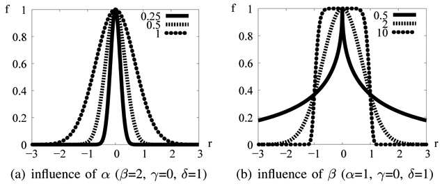
1D generalized Gaussian function f (r; α, β, γ, δ)

• α is the parameter modeling lesion size

• β is the parameter modeling lesion sharpness: it is a shape factor (the same value is used for each lesion in images of the same modality)

• γ is the parameter modeling the background intensity

• δ is the parameter modeling lesion height

As an illustration, some typical MA images and corresponding profiles are shown in figure 3(a) and compared to a synthetic lesion generated by the model. The generalized Gaussian function is convenient as it can model a wide range of shapes. Thus, it can model MAs with more or less sharp outlines, depending on imaging modality.

Fig. 3.

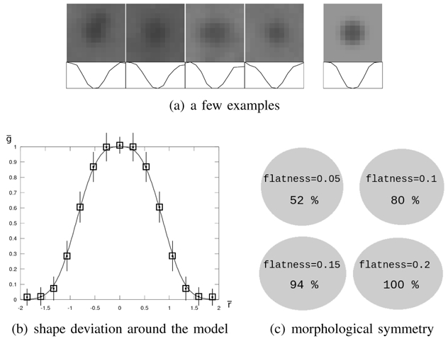
Microaneurysm model validation. In figure (a), four examples of microaneurysms (on the left) and the model (on the right) are displayed together with image profiles. Figure (b) reports the mean and standard deviation of the pixel-wise estimation error, given in table II. The mean for each interval is represented by a square, and standard deviations by line segments: the length of a half segment corresponds to the standard deviation. And finally, figure (c) illustrates the distribution of flatness among microaneurysms: four ellipses with different flatnesses are displayed together with the percentage of manually delimited lesions of greater flatness.

To validate the model relevance, we studied the shape deviation between real MAs and the model. To this end, 100 reference lesions were selected at random in the analyzed images. For each lesion, α, γ and δ were estimated to match locally the lesion, given a constant shape factor β = β₀. Image backgrounds were determined by using operators from mathematic morphology (opening and closing of size 15), and removed from images prior to parameter estimation (this preprocessing step was performed to validate the model only). For each lesion, α was determined from a discrete set of values {α₁,…, α_n}: for each tested value α_i, γ and δ were estimated from the pixels found at a distance from the lesion center of less than 2α_i (roughly the lesion area). Let g be a pixel gray level, $\overline{g}=\frac{g-\gamma }{\delta }$ the normalized gray level, r the distance from that pixel to the lesion center, $\overline{r}=\frac{r}{\alpha }$ the normalized distance and ē_pw = ḡ − f(r̄; 1, β₀, 0, 1) the pixel-wise estimation error. To determine β₀, we estimated α, γ and δ for each lesion with several values for β₀ and we kept the value that minimized the sum over r̄ of the mean ē_pw. We then studied the mean and standard deviation of ē_pw according to the distance from the lesion center r̄. Results are given in table II and figure 3(b) for color photographs and an optimal value β₀ = 4. It emerged that the mean estimation error was very low for any distance from the lesion center, even if the standard deviation was rather high.

TABLE II. Shape deviation between real microaneurysms and the model.

distance interval	mean	standard deviation
0 ≤ r ≤ r0	−0.0099	0.085
r0 ≤ r ≤ r1	0.0177	0.144
r1 ≤ r ≤ r2	0.0101	0.152
r2 ≤ r ≤ r3	0.0081	0.159
r3 ≤ r ≤ r4	−0.0135	0.154
r4 ≤ r ≤ r5	−0.0215	0.123
r5 ≤ r ≤ r6	0.0023	0.095
r6 ≤ r ≤ 2α	0.0141	0.086

Mean and standard deviation of the pixel-wise estimation error, expressed in pixels, for several intervals of distance r from the lesion center, ranging from r = 0 to r = 2α. These results are reported in figure 3(b).

To show the relevance of a rotation-symmetric model, the 100 reference lesions were manually delimited with an elliptical shape by the expert. Then, the flatness coefficient of ellipses (one minus the ratio between the minor and the major axes) was computed: the results are reported in figure 3(c). They confirmed that most MAs are almost round and that they are never very flat.

C. Template-matching in the Wavelet Domain

1) Template-matching: usually, to perform template-matching in an image I, we move a window w over I and consider the subimages of I defined by the positions of w, noted I_|w (examples are given in figure 4). To classify the content of I_|w, we have to find the set of parameters (in our case: (α, γ, δ), β₀ is given - see equation (1)) for which the parametric model best matches I_|w. If the model is close enough to I_|w, a lesion is detected at the center of w. The distance measure commonly used is the sum of the squared errors (SSE): it is defined as the sum of the squared differences between the value of each pixel of I_|w and the corresponding value of the model function.

Fig. 4.

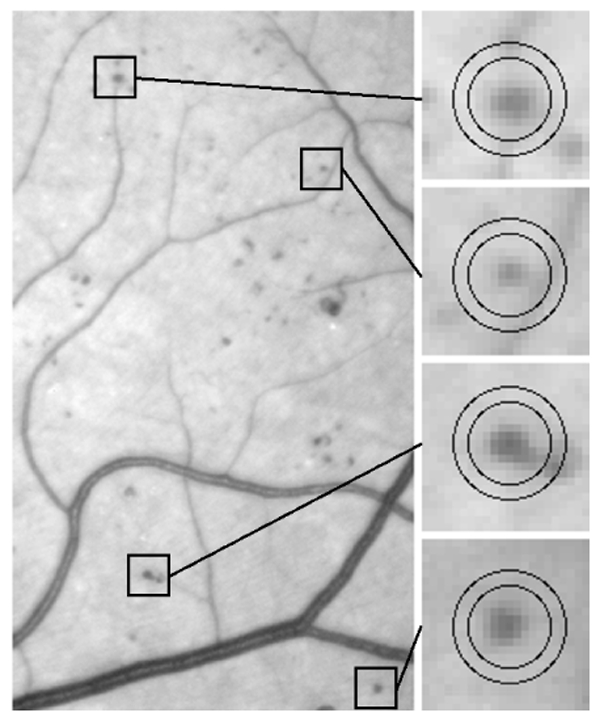
Examples of microaneurysms within moving windows. The microaneurysm detector tries to match models with n = 2 different values for α; a different moving window is used for each value of α. The two windows matching each example are shown in the figure.

2) Adaptation in the Wavelet Domain: the wavelet decomposition of an image produces several subimages of coefficients (called subbands), each of them containing information at a specific scale/frequency and along a specific direction (see figure 5(a)). These subbands contain more or less relevant information to describe MAs. We propose adaptation of the previous procedure in the wavelet domain, to subbands that contain discriminant information alone. In particular, by ignoring high and low frequency subbands, we can get rid of noise and slow image variations, respectively. Moreover, the wavelet transform of g = f − γ, where f is the model function and γ is the local background intensity, differs from the wavelet transform of f only in the lowest frequency subband. Thus, if we reject the lowest frequency subband, the offset parameter γ can be set to 0: as a conclusion, the model can be defined in the spatial domain by only 3 parameters (α, β₀ and δ).

Fig. 5.

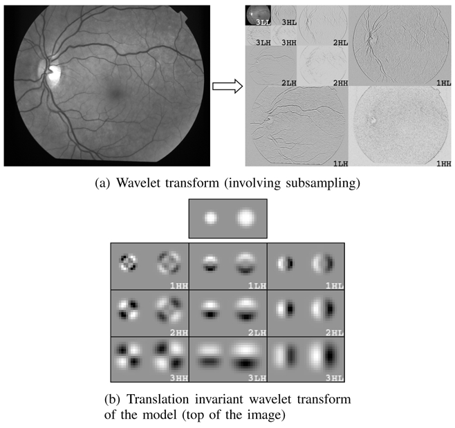
The wavelet transform. In both figures (a) and (b), there are three subbands at each scale, depending on whether the rows/columns were high-passed or low-passed filtered. In these examples, the number of decomposition levels is 3 (Nl = 3). In the wavelet transform images, positive values are represented in white, negative values in black. In image (b), two microaneurysm models with different values for α are decomposed.

In the proposed method, for n predetermined standard deviations α_i, the normalized model f(r; αi, β₀, γ = 0, δ = 1) is discretized and its wavelet transform WTM_i is computed. Let J be the set of discriminant subbands. The SSE is now defined as the sum of the squared differences between the coefficients of WTI_|w (the wavelet transform of I restricted to the window w) divided by δ_i and that of WTM_i, in the subbands of J (δ ↦ f(r; α_i, β₀, γ = 0, δ) is linear and the wavelet transform is linear). The proposed procedure is summarized as follows:

• For each standard deviation α_i, 1 ≤ i ≤ n, we compute the lesion height δ_i minimizing the SSE between WTM_i and $\frac{WT{I}_{\mid w}}{{\delta }_i}$ (δ_i is computed by the least mean squared algorithm).

  • - If δ_i is not in a predetermined range of values, no lesions of size α_i are detected in I_|w.

  • - Otherwise, I_|w is classified as a MA of size α_i and height δ_i if the SSE is below a corresponding threshold t_i ∈ T, 1 ≤ i ≤ n.

The set of discriminant subbands J, the standard deviations α_i and the thresholds t_i are learnt, as we will explain in sections II-E2 and II-E3.

3) Moving windows: it is assumed that a moving window contains at most one lesion. Problems might occur if a lesion is too close to another lesion or to a vessel (see figure 4). As a consequence, we had to use small moving windows: we used circular windows of radius 2α_i (see section II-B). It is not necessary to move the windows to each pixel location: the moving step is chosen in inverse proportion to the typical lesion size. In our images, we evaluated $\frac{L}{4}$ window positions, where L is the number of image pixels. To speed up the search, we do not evaluate areas I_|w where max(I_|w) − min(I_|w) is below the range of values for δ.

D. Wavelet Adaptation to our Specific Problem

Wavelet transform is highly tunable and we have a free choice of the function basis used to decompose images. So we propose a search for a wavelet basis which may make matched filtering in the wavelet domain easier and more efficient. However, the design of matched wavelet bases is usually a difficult task, as several constraints have to be satisfied simultaneously (such as biorthogonality, regularity, vanishing moments, etc) [25]. Many constructions of wavelets have been introduced in the mathematical [26] and signal processing literature (in the context of quadrature mirror filters) [27], to satisfy those constraints. Moreover, these properties might not be sufficient to process specific signals or images. Thus, several studies have been carried out to adapt a wavelet to a signal of reference, with different constraints on the wavelet properties and on the adaptation criteria. Usually, the goal is to minimize the L² norm between the signal and an approximation derived from its wavelet decomposition (for compression purposes, for instance) [22][28]. These methods have been applied to medical classification problems, in order to match waveform signals [29][30]. However, in our case, we do not intend to match a signal of reference, which is not relevant as the lesions we study present great variations in size and amplitude. We look for the basis best adapted to our problem: template matching in the wavelet domain. The only criterion available is the system’s overall classification rate. So we have to design a wavelet empirically, by a numerical optimization procedure, in which no explicit expression of the wavelet fitness function is given.

In 1994, Sweldens introduced a convenient way to satisfy all the desired properties of wavelets by reducing the problem to a simple relation between the wavelet and scaling coefficients. This approach, named the lifting scheme [31], makes it possible to relax all the mentioned constraints and thus to reach a simple optimization process. Indeed, it is possible to generate any compactly supported biorthogonal wavelet with a compactly supported dual. A filter bank was proposed in [25] to implement the lifting scheme (see figure 6). It defines two linear filters, named predict (P) and update (U). U and P are two real vectors, respectively of size N_p and N_u. The coefficients of those filters have only to satisfy two linear relations to generate biorthogonal wavelets (see appendix A). They allow a perfect reconstruction of decomposed images. Moreover, the lifting scheme makes the wavelet transform faster, and is used in the Jpeg-2000 compression standard [32]. For these reasons, we decided to design lifting scheme based wavelet filters to transform our images.

Fig. 6.

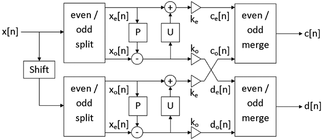
Two-channel filterbank for the translation invariant wavelet transform within the lifting scheme framework. k_e and k_o normalize the energy of the underlying scaling and wavelet coefficients.

In addition to the wavelet basis, the wavelet transform enabled us to choose the subbands in which images are decomposed, by selecting at each scale which subbands are further decomposed. An algorithm, called “best basis”, has been proposed by Coifman [33] [34] to match such a subband selection to a given family of signals. Nevertheless, this approach is too restrictive for the proposed algorithm, since the decomposition on the best basis preserves all the information contained in the images, whereas we want to reject irrelevant information (such as noise). So, we explored the entire space of subband subsets, in order to find the best ones, from the overall classification rate point of view. Finally, we did not subsample subbands in the usual way in the wavelet transform. Because the typical size of MAs is small in our images (the average diameter is about 10 pixels), we decided to use the translation invariant wavelet transform [35], in which every subband is the size of the raw image (see also appendix A). The models and an example of translation invariant decomposition are shown in figure 5(b).

E. Description of the Calibration Procedure

1) Overall Procedure (figure 7(a)): to calibrate the proposed classifier, we had several parameters to determine. These parameters were learnt from a subset of the analyzed images: the learning dataset. The remaining analyzed images (the validation dataset) were only used to evaluate the whole algorithm, when parameter selection had been accomplished. The number of images required in the learning dataset is discussed in section III. We classified the parameters into three groups:

Fig. 7.

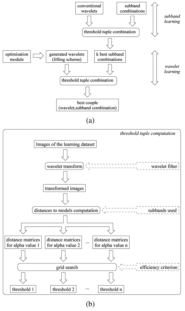
Overall learning procedure

• The model parameters (n values for α, a range of values for δ, a value for β, see equation (1))

• The decomposition subband subsets used to compute the SSE: we had 3 × N_l + 1 binary values to set, where N_l is the maximum number of decomposition levels considered. For our images, we set N_l to 3, because our experiments show that there is no interest in decomposing on more than three levels: information at lower frequencies is not adapted to MA scale. Let S = {1HH, 1HL, 1LH, 2HH, 2HL, 2LH, 3HH, 3HL, 3LH, 3LL} be the set of available subbands (see figure 5). We had to evaluate each subset J_m ∈ 2^S\∅, 1 ≤ m ≤ M (where 2^S is the set of subsets of S, M = card(2^S\∅) = 2^card(S) − 1 = 1023).

• The wavelet filter support and coefficients: we evaluated both conventional and specific adapted wavelets (based on the lifting scheme)

Groups of parameters were defined in a specific order, which is discussed hereafter. Model parameters are obviously independent from the wavelet filter and the subband subset selection, therefore, they were calibrated first. A more difficult issue is whether the wavelet filters and the subband subsets should be learnt simultaneously, which would be an extremely time-consuming process. To simplify the learning procedure, the subband subsets were evaluated first with several conventional wavelets. These evaluations provided the best subband subsets, which were then used to learn the adapted wavelet filters. The learning procedure can be summarized as follows:

1. model parameter selection (see section II-E3)

2. subband subset learning (see section II-E4)

3. wavelet learning (see section II-E5)

To determine the subband subsets and the adapted wavelets, we needed to compute the n thresholds on the SSE (one for each value of α) each time we evaluated a couple (wavelet, subband subset). The method is explained in the following section.

2) Computation of the Thresholds on the SSE for a Couple (wavelet filter Wj, subband selection J_m): according to section II-C, we had to learn a threshold t_t for each value of α_i, 1 ≤ i ≤ n (the model standard deviations). Elements of the threshold tuple T = (t₁, t₂, …, t_n) were determined simultaneously. First, each image I in the learning dataset was decomposed with W_j and the resulting subbands in J_m were stored. Then the SSE were computed at each corresponding position in J_m of the sliding window w on these images, for each value of α_i (see equation (1)). A classification score was defined (equation (3) -see explanation below). We wanted to know which T provided the best classification score, according to the manual detections provided by the expert. This was done by a simple grid search optimization: we explored the space of T with a given step and retained the best. The procedure is illustrated in figure 7(b).

To define the classification score, it is important to notice that, when optimizing T, we actually have two fitness criteria: sensitivity (the percentage of lesions that are detected) and PPV (Positive Predictive Value: the percentage of relevant detections). We considered a detected object relevant if the ground truth indicated a lesion centerpoint within three pixels (as a comparison, the average lesion radius is five pixels). Sensitivity and PPV may be conflicting, then optimization involves finding the best compromise between the two objective scores. In [36], the authors proposed to combine sensitivity and PPV following equation (2).

$$\mathit{score}=\sqrt{\mathit{sensitivity}\times \mathit{PPV}}$$ (2)

Thus, score is high if and only if both sensitivity and PPV are high. However, in a disease screening framework, the cost of false negatives is higher than that of false positives. Indeed, it is better to send a healthy patient to an ophthalmologist for further analyses, than to miss lesions, and let an ill patient leave without treatment. If we use that fitness score, we observe that PPV is favored. Therefore we decided to penalize threshold tuples for which sensitivity is lower than PPV by using the following score definition (equation (3)).

$$\{\begin{array}{l}\mathit{score}=\zeta \left(\frac{\mathit{sensitivity}}{\mathit{PPV}}\right)\times \sqrt{\mathit{sensitivity}\times \mathit{PPV}}\hfill \\ \zeta (x)=x\mathit{for}x<1,\zeta (x)=1\mathit{otherwise}\hfill \end{array}$$ (3)

3) Model Parameter Selection: the choice of β is explained in section II-B. Ranges for amplitudes δ were determined on 100 reference lesions so that every sample laid within them. Finally, the standard deviations α, the most critical parameters, were learnt from all the analyzed images. They were chosen so that the template-matching classification score was maximized. This procedure was performed taking different numbers n of values for α: it emerged from all the trials that the use of n = 3 values did not bring any significant improvement over n = 2. For instance, if the Haar wavelet was used to decompose images, sensitivity increased by 6.56% when n increased from 1 to 2 and by 0.17% when it increased from 2 to 3.

4) Subband Subset Learning: we wanted to select a few subband subsets that would be used to compute the SSE, regardless of the wavelet used to decompose images. We assumed that the subband subsets that work best together with several conventional wavelets are liable to be the most efficient with any other wavelet. To select them, we evaluated each subset J_m ∈ 2^S\∅, 1 ≤ m ≤ M with N conventional wavelets. The N = 4 wavelets we used are given below with their support (lowpass filter support/highpass filter support):

• the orthogonal Haar wavelet (support=2/2): W₁

• the Le Gall 5/3 biorthogonal wavelet, which is used in the Jpeg2000 standard part I [37] (support=5/3): W₂

• the Daubechies 9/7 biorthogonal wavelet, also in the Jpeg2000 standard (support=9/7): W₃

• the Daubechies 4-tap orthogonal wavelet [38] (support=4/4): W₄

For each subset J_m and each conventional wavelet W_i, 1 ≤ i ≤ N, we computed the score of the couple (W_j, J_m), defined as the score obtained for the best threshold tuple (see section II-E2). The global score, on all the wavelets, of each J_m is given by equation (4).

$$\mathit{score}(J_m)=\frac{1}{N}\sum _{i=1}^N\mathit{score}(W_i,J_m)$$ (4)

Then we kept the k best subband subsets ( $J_1^{\mathit{opt}},J_2^{\mathit{opt}},\dots ,J_k^{\mathit{opt}}$), defined as the subsets with upper score.

5) Wavelet Learning: For each of the best subband configurations $J_i^{\mathit{opt}}$, 1 ≤ i ≤ k, we searched for the best couple (lifting scheme based designed wavelet, $J_i^{\mathit{opt}}$). Within the lifting scheme, predict and update filters have non-zero even filter lengths [25]. As a result, by reference to formula 13 (appendix A), the corresponding wavelet filters can have the following supports:

• 5/3 (N_p = 2, N_u = 2 → 2 parameters)

• 9/3 (N_p = 2, N_u = 4 → 4 parameters)

• 9/7 (N_p = 4, N_u = 2 → 4 parameters)

• 13/7 (N_p = 4, N_u = 4 → 6 parameters)

• or larger

As we are studying small structures, we considered only the first three filter configurations.

A meta-algorithm was used to generate lifting scheme based wavelets (see appendix B). Each time a wavelet W was generated, it was evaluated jointly with one of the k best subband subsets on the learning dataset, using the procedure described in section II-E2.

III. RESULTS

The algorithm parameters and wavelet filter coefficients obtained for each imaging modality are given in table III. The influence of standard deviations α (see equation (1)) on the classification score is illustrated in figure 8.

TABLE III. Algorithm and wavelet filter parameters for each imaging modality.

group	parameters	GFC photo.	Color photo.	Angiographs	scaling filter	wavelet filter
Model	sign	−1	−1	1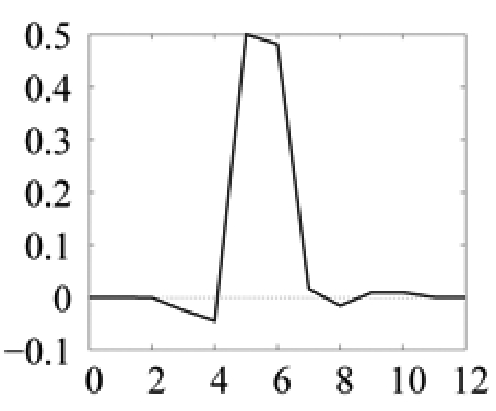
	β	4	4	3
	α (small model)	2.263	2.316	2.316
	δ (small model)	20%–45%	20%–45%	20%–80%
	α (large model)	3.526	2.947	3.263
	δ (large model)	25%–55%	25%–55%	60%–140%
Adapted Wavelet	filter support	5/3	9/3	9/3
	predict filter	[0.041;0.959]	[0.030;0.970]	[−0.039;1.039]
	update filter	[0.462;0.038]	[0.000;0.500; 0.000;0.000]	[−0.025;0.500; 0.016;0.009]
Subbands	set	{2HL,2LH}	{2HL,2LH}	{2HL,2LH}
Thresholds	small model	5.86×10−3	5.79 ×10−3	5.02×10−3
	large model	3.19×10−3	3.94×10−3	3.10×10−3

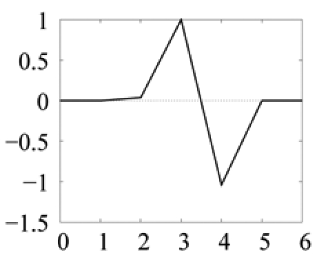
The sign parameter indicates whether the generalized Gaussian is upside down (−1) or not (1). Amplitude (δ) ranges are given as a percentage of the mean image intensity and model sizes (α) are given as a number of pixels. Predict and update filters define the filter bank implementing the lifting scheme (see procedure in figure 6). As an illustration, the corresponding scaling filter and wavelet filter for color photographs are plotted below (the connection between the two filter representations is explained in [25]). Thresholds on SSE are defined on normalized SSE values: SSE values, computed for normalized wavelet functions, are divided by the number of pixels in (WTM_i)_|w.

Fig. 8.

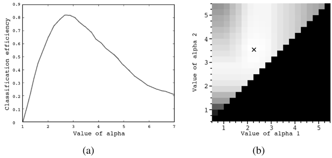
Influence of the generalized Gaussian function standard deviation on the classification score. Figure (a) shows the classification score according to the standard deviation α in the case n = 1 (when template matching is performed with a single model size). Figure (b) shows the classification score according to the couple of standard deviations (α₁,α₂), α₁ < α₂, in the case n = 2. Classification scores are proportional to the gray level and the optimal couple is represented by a cross.

An important question we had to answer, was the number p of images required in learning sets. We noticed that only three images per imaging modality database are necessary to learn the n = 2 thresholds on the SSE (one for each value of α), given a wavelet filter, a subband selection and the model parameters (see table IV). Thus the calibration score (the score computed in learning sets) is approximately equal to the test score (the score computed in validation sets). However, when searching for the optimal subband selection (on conventional wavelets) or for the optimal wavelet filter, given a subband selection (see procedure in figure 7(a)), the number of parameters increases. To determine p, we applied the learning process of section II-E with an increasing number p until the test error stopped evolving. Whatever images we chose in the learning set, the test error stopped evolving for p = 8 at most. The choice of p had little correlation with the number of lesions in images. In any case, with too few lesions (less than 40), the objective function (equation (3)) is discontinuous and parameter estimation becomes imprecise. For each imaging modality, we used 8 images in the learning set. The best subband subsets are given in figure 9. We give the score of conventional wavelets with the first three subsets in table V(a). Results clearly show that the efficiency of the method depends on the wavelet used, which confirms the interest of looking for an optimal wavelet. However, as stated above, optimal subband combinations depend little on the wavelet filter used.

TABLE IV. Learning and validation scores with an example.

set	modality	GFC photo.	Angiographs	Color photo.
L	nr. of images	3	3	3
	nr. of lesions	215	231	39
	sensitivity	88.62%	93.81%	83.62%
	PPV	87.74%	92.11%	83.61%
V	nr. of images	47	32	32
	nr. of lesions	2793	2521	761
	sensitivity	87.97%	93.32%	82.94%
	PPV	86.88%	91.07%	82.58%

Score values computed on the learning set (L) and the validation set (V) for the Haar wavelet on the following subband subset: {2HL, 2LH}.

Fig. 9.

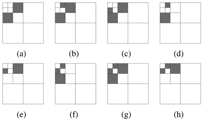
Best combinations of subbands for template matching using conventional wavelets. The first 8 best combinations in decreasing order of their scores (from (a) to (h)). It emerges that the highest frequency subbands (1HH, 1HL, 1LH) and the lowest (3LL), as well as the diagonal subbands (1HH, 2HH, 3HH) are not used (see figure 5 for the subband names).

TABLE V. Classification efficiency according to the subband selection.

(a) Conventional wavelets
	subbands	Haar wavelet	5/3 biorthogonal wavelet	4-tap orthogonal wavelet	9/7 biorthogonal wavelet
GFC photo.	{2HL, 2LH}	(87.97%,86.88%)	(75.48%,74.41%)	(72.88%,71.76%)	(69.77%,66.57%)
	{2HL, 2LH, 3HL}	(78.88%,76.69%)	(71.37%,67.17%)	(38.52%,37.92%)	(63.93%,60.44%)
	{2HL, 2LH, 3LH}	(78.56%,75.69%)	(71.05%,67.20%)	(38.72%,34.34%)	(62.97%,60.82%)
Angiographs	{2HL, 2LH}	(93.32%, 91.07%)	(83.71 %,80.25%)	(80.04%,79.36%)	(84.62%,81.26%)
	{2HL, 2LH, 3HL}	(85.82%,83.53%)	(84.80%,85.31%)	(61.86%,61.80%)	(82.23%,81.86%)
	{2HL, 2LH, 3LH}	(85.91%,84.18%)	(84.62%,84.84%)	(62.97%,60.98%)	(81.45%,80.82%)
Color photo.	{2HL, 2LH}	(82.94%,82.58%)	(71.18%,66.60%)	(64.09%,62.08%)	(60.44%,58.51%)
	{2HL, 2LH, 3HL}	(74.73%,75.14%)	(74.18%,68.53%)	(34.62%,27.04%)	(66.48%,60.20%)
	{2HL, 2LH, 3LH}	(69.23%,66.32%)	(74.18%,67.84%)	(29.67%,29.35%)	(68.13%,59.90%)
(b) lifting scheme based wavelets
		subbands	5/3	9/3	9/7
GFC photo.		{2HL, 2LH}	(90.24%, 89.75%)	(87.03%,88.44%)	(89.83%,89.41%)
		{2HL, 2LH, 3HL}	(88.32%,88.06%)	(87.72%,87.63%)	(87.35%,87.57%)
		{2HL, 2LH, 3LH}	(87.41%,87.43%)	(87.89%,87.50%)	(87.48%,87.38%)
Angiographs		{2HL, 2LH}	(89.38%,91.50%)	(93.74%,91.67%)	(91.29%,89.70%)
		{2HL, 2LH, 3HL}	(88.95%,88.87%)	(88.94%,88.67%)	(87.89%,87.53%)
		{2HL, 2LH, 3LH}	(87.86%,87.96%)	(88.11%,87.79%)	(87.64%,87.42%)
Color photo.		{2HL, 2LH}	(87.80%,88.60%)	(89.62%,89.50%)	(89.18%,88.94%)
		{2HL, 2LH, 3HL}	(87.48%,87.43%)	(85.84%,86.59%)	(86.72%,86.71%)
		{2HL, 2LH, 3LH}	(87.08%,86.81%)	(86.26%,86.19%)	(86.66%,86.72%)

In each cell, the classification scores are given as a couple (sensitivity, PPV). Values are computed on the validation dataset.

Classification scores obtained for optimally designed wavelets are given in table V(b) and the optimal couples (wavelet filter, combination of subbands) found for each imaging modality database have already been given in table III. In figure 10, we gave an example of manually and automatically processed GFC image.

Fig. 10.

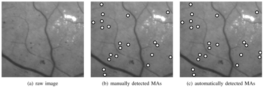
Example of green filtered photograph: (a) original image, (b) analysed image, (c) processed image. There is a false positive detection (right border).

Finally, the proposed method (PM) was compared with those introduced by Fleming [9] and Niemeijer [14] in our database, using the same learning and validation sets. These methods were implemented following the description in the literature, where they are designed to process color photographs. We adapted them to each of the three imaging modalities to handle differences in image resolution, number of color planes, color and typical size of vessels and lesions. In particular, features extracted from the blue, red and hue image planes are ignored when processing gray level images, and vessel or lesion dependent parameters are tuned to maximize the classification score. We also evaluated our lesion detector as a candidate extractor for Niemeijer’s method (NPM), instead of mathematical morphology and pixel classification based candidate extractors. With this aim, the thresholds on the SSE were learnt so that at least 98% of the lesions in the learning set were detected (by analogy with the pixel classification based candidate extractor), with as few false positives as possible (the other parameters are set to the values of table in). The classification scores are given in table VI.

TABLE VI. Comparison of the proposed method with Fleming’s and Niemeijer’s method.

method	GFC photo.	Angiographs	Color photo.
PM	(90%,90%)	(94%,92%)	(90%,89%)
Fleming	(68%,68%)	(81%,77%)	(70%,55%)
Niemeijer	(69%,73%)	(80%,79%)	(57%,61%)
NPM	(73%,73%)	(79%,85%)	(61%,58%)

Results are given as optimal couples (per lesion sensitivity, per lesion PPV) on the validation dataset.

IV. DISCUSSION

In this study, we have proposed a new method for detecting MAs in the retina, based on template-matching in the wavelet domain. The wavelet basis is adapted using the lifting scheme framework. A new criteria has been proposed to evaluate a lesion detector (see equation (3)): it makes it possible to search for the wavelet basis, the relevant subbands and the template-matching parameters in an automatic fashion. The results show that individual lesions can be detected with both a high sensitivity and a high positive predictive value for different photographic modalities. Thus a sensitivity/PPV pair of (90.24%,89.75%) was achieved for GFC photographs, of (93.74%,91.67%) for angiographs and of (89.62%,89.50%) for color photographs. According to that criterion, this method outperforms recent publications [9][14] about MA detection. Moreover, the method is quite insensitive to quality variation between images (see figure 11 for instance). The wavelet filter used for decomposition has been designed by an optimization process within the lifting scheme framework, with the classification rate as the fitness criterion. Wavelet adaptation notably improves the results obtained by conventional wavelet filters. This is particularly true for color photographs: we observe an improvement of 6.7% in sensitivity and of 6.9% in PPV (see tables V(a) and (b)). Wavelet filters (resp. scaling filters) obtained by the calibration procedure are almost antisymmetric (resp. symmetric), like Haar wavelet/scaling filters and unlike the other wavelets filters we studied. Precisely, for Haar and the adapted wavelet, the scaling filter looks roughly like MAs. This explains why the Haar wavelet gives better results than the others (table V(a)). Indeed, if the scaling function matches MA at a given scale j, information specific to MAs is concentrated in subbands of scale j. Thus template-matching can be performed in those subbands alone: relevant and irrelevant information has been decorrelated. Since MAs are rotation-invariant, as discussed in section II-B, MA specific information lies equally in both horizontal (j₁HL) and vertical (j₂LH) subbands. This can be seen in figure 9: each of the best subband selections include both an horizontal and a vertical subband, either at the second or at the third decomposition level.

Fig. 11.

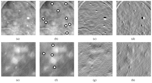
Examples of good quality (a) and blurred image (e): the algorithm works well on both examples with the same set of parameters. Two areas containing microaneurysms from different images are displayed with their optimal wavelet transform (the subbands used by the WTM only). These images are angiographs. As a consequence microaneurysms are white. Images have been enhanced, so some microaneurysms seem to have homogeneous values. They were processed with the same set of parameters. Each row corresponds to an image. (a),(e): raw images, (b),(f): automatic detection (which matches the manual detection), (c),(g): vertical decomposition subband considered, (d),(h): horizontal decomposition subband considered.

Some problems are not completely solved by the method. Firstly, a few MAs are not detected because they are too close to big vessels or clustered. A solution to these problems might be vessel elimination and iterative lesion elimination, respectively. Secondly, some punctiform hemorrhages (another lesion of DR) are detected as MAs, as well as dust stuck to camera lenses or some small structures that ophthalmologists have difficulty to differentiate from MAs.

The proposed method is fast: the learning step is processed only once; then the detection process consists in only two steps: wavelet transform and template-matching. It does not require extracting and classifying candidates. The total time required to process a single image, of definition 1280 pixels/line for 1008 lines/image, is approximately 2 seconds on a 2 GHz AMD Athlon 64-bit processor. The method can also be used as an efficient candidate extractor and be coupled with a candidate classification method. It is also interesting in terms of reproducibility because parameter estimation is performed automatically and images do not need acquisition-specific preprocessing. Given its simplicity and reproducibility, this method may be one of the answers for disease follow up. Moreover, the method can be adapted to other structures in the retina (like vessels with directional models, or punctiform hemorrhages for instance).

In the current study, we processed images from different modal­ities separately. We are now processing series of multimodal registered images to fuse their complementary information, for patient follow up.

Appendix A The Lifting Scheme

A multiresolution approximation is a nested sequence of linear spaces (V_j)_{j ∈ ℤ} for approximating functions f ∈ L₂(ℝ) such that:

• V_j ⊂ V_j+1, ∀_j ∈ ℤ

• ${\displaystyle \underset{j=-\infty }{\overset{+\infty }{\cup }}}{V}_j$ is dense in L₂ (ℝ) and ${\displaystyle \underset{j=-\infty }{\overset{+\infty }{\cap }}}{V}_j=\{0\}$

• f(x) ∈ V_j ⇔ f(2x) ∈ V_j+1, ∀_j ∈ ℤ

• f(x) ∈ V_j ⇒; f(x − 2^−k) ∈ V_j, ∀_j, k ∈ ℤ

The approximation of a function f ∈ L₂(ℝ) at a resolution 2^j is defined as the projection of f on V_j. There is a function Φ ∈ L₂(ℝ), called scaling function, such that for any j ∈ ℤ, ${(x\mapsto {\mathrm{\Phi }}_{jk}(x)=\sqrt{2^j}\mathrm{\Phi }(2^{j}x-k))}_{k\in \mathbb{Z}}$ is a basis of V_j. The scaling function Φ satisfies the refinement relation of equation (5).

$$\mathrm{\Phi }(x)=2\sum _{k=-\infty }^{\infty }{h}_k\mathrm{\Phi }(2x-k)$$ (5)

The additional information available in the approximation of f at the resolution 2^j+1 as compared with the resolution 2^j, is given by the projection of f on the orthogonal complement of V_j in V_j+1, noted W_j. There is a function Ψ ∈ L₂(ℝ), called wavelet function, such that for any j ∈ ℤ, ${(x\mapsto {\mathrm{\Psi }}_{jk}(x)=\sqrt{2^j}\mathrm{\Psi }(2^{j}x-k))}_{k\in \mathbb{Z}}$ is a basis of W_j. The wavelet function Ψ satisfies the refinement relation of equation (6).

$$\mathrm{\Psi }(x)=2\sum _{k=-\infty }^{\infty }{g}_k\mathrm{\Phi }(2x-k)$$ (6)

{V_j}_{j ∈ ℤ} and {W_j}_{j ∈ ℤ} constitute what we call a multiresolution analysis framework. We define a dual multiresolution analysis framework ({Ṽ_j}_{j ∈ ℤ},{W̃_j}_{j ∈ ℤ}) associated with a dual scaling function Φ̃ and a dual wavelet function Ψ̃, that are biorthogonal to Φ and Ψ (see equation (7)).

$$\{\begin{array}{l}<{\stackrel{\sim }{\mathrm{\Phi }}}_{jk},{\mathrm{\Phi }}_{j{k}^{\prime }}>={\delta }_{k{k}^{\prime }}\hfill \\ <{\stackrel{\sim }{\mathrm{\Psi }}}_{jk},{\mathrm{\Psi }}_{j{k}^{\prime }}>={\delta }_{k{k}^{\prime }}\hfill \\ <{\stackrel{\sim }{\mathrm{\Psi }}}_{jk},{\mathrm{\Phi }}_{j{k}^{\prime }}>=0\hfill \\ <{\stackrel{\sim }{\mathrm{\Phi }}}_{jk},{\mathrm{\Psi }}_{j{k}^{\prime }}>=0\hfill \end{array}$$ (7)

Φ̃ and Ψ̃ satisfy refinement relations such as (5) and (6) with coefficients h̃_k and g̃_k respectively. A function f ∈ L₂(ℝ) can be written as follows:

$$\begin{array}{l}x\mapsto f(x)=\sum _{j,k\in \mathbb{Z}}<f,{\stackrel{\sim }{\mathrm{\Psi }}}_{j,k}>{\mathrm{\Psi }}_{j,k}(x)\\ =\sum _{k\in \mathbb{Z}}<f,{\stackrel{\sim }{\mathrm{\Phi }}}_{J,k}>{\mathrm{\Phi }}_{J,k}(x)\\ +\sum _{j\le J,k\in \mathbb{Z}}<f,{\stackrel{\sim }{\mathrm{\Psi }}}_{j,k}>{\mathrm{\Psi }}_{j,k}(x),J\in \mathbb{Z}\end{array}$$ (8)

The lifting scheme allows the construction of compactly supported wavelets with compactly supported duals, i.e. such that the refinement filters h_k, g_k, h̃_k and g̃_k are finite filters (a finite number of coefficients are non-zero). We define the following 2π-periodic functions $h(\omega )={\sum }_{k=-\infty }^{\infty }{h}_k{e}^{-ik\omega }$ and $g(\omega )={\sum }_{k=-\infty }^{\infty }{g}_k{e}^{-ik\omega }$ and the following matrices (called modulation matrices) $m(\omega )=\left(\begin{array}{cc}h(\omega )& h(\omega +\pi )\\ g(\omega )& g(\omega +\pi )\end{array}\right)$ and $\stackrel{\sim }{m}(\omega )=\left(\begin{array}{cc}\stackrel{\sim }{h}(\omega )& \stackrel{\sim }{h}(\omega +\pi )\\ \stackrel{\sim }{g}(\omega )& \stackrel{\sim }{g}(\omega +\pi )\end{array}\right)$. A necessary condition for biorthogonality, which ensures perfect reconstruction, is given in equation (9).

$$\forall \omega \in ℝ:\stackrel{\sim }{m}(\omega )\overline{m^t(\omega )}=1$$ (9)

In the case of finite filters, det(m(ω)) is a monomial, the determinant is chosen as det(m(ω)) = −e^−iω which leads to (10):

$$\{\begin{array}{l}\stackrel{\sim }{g}(\omega )=e^{-i\omega }\overline{h(\omega +\pi )}\hfill \\ g(\omega )=e^{-i\omega }\overline{\stackrel{\sim }{h}(\omega +\pi )}\hfill \\ \overline{h(\omega )}\stackrel{\sim }{h}(\omega )+\overline{h(\omega +\pi )}\stackrel{\sim }{h}(\omega +\pi )=1\hfill \end{array}$$ (10)

The lifting scheme relies on a simple relationship between all multiresolution analysis frameworks that share the same scaling function: let {Φ⁰, Φ̃⁰ Ψ⁰, Ψ̃⁰} be an initial set of biorthogonal scaling and wavelet functions, then a new set { Φ, Φ̃, Ψ, Ψ̃} can be found according to equation (11)[31].

$$\{\begin{array}{l}\mathrm{\Phi }(x)={\mathrm{\Phi }}^0(x)\hfill \\ \mathrm{\Psi }(x)={\mathrm{\Psi }}^0(x)-{\sum }_k{s}_k{\mathrm{\Phi }}^0(x-k)\hfill \\ \stackrel{\sim }{\mathrm{\Phi }}(x)=2{\sum }_k{\stackrel{\sim }{h}}_k^0\stackrel{\sim }{\mathrm{\Phi }}(2x-k)+{\sum }_k{s}_{-k}\stackrel{\sim }{\mathrm{\Psi }}(x-k)\hfill \\ \stackrel{\sim }{\mathrm{\Psi }}(x)=2{\sum }_k{\stackrel{\sim }{g}}_k\stackrel{\sim }{\mathrm{\Phi }}(2x-k)\hfill \end{array}$$ (11)

Coefficients s_k of equation (11) can be freely chosen. Hence we can start with an initial set of biorthogonal filters and generate new biorthogonal filters by the previous relation.

In [25], the authors propose a filter bank adapted from equation (11). It uses the lazy wavelet [31] as initial biorthogonal filter and two filters P and U are defined from the s_k coefficients. The lazy wavelet is the set of biorthogonal filters given in equation (12):

$$\{\begin{array}{l}2{\stackrel{\sim }{h}}^0(\omega )=h^0(\omega )=1\hfill \\ {\stackrel{\sim }{g}}^0(\omega )={2_g}^0(\omega )=e^{-i\omega }\hfill \end{array}$$ (12)

One step in the lazy wavelet transform consists in splitting the signal into its odd and even indexed samples. In the case of the decimated wavelet transform, one step of the wavelet decomposition is given as follows:

• split: the signal x[n] is split into its odd x₀[n] and even x_e[n] coefficients.

• predict: we generate the wavelet coefficients d[n] as the error in predicting x₀[n] from x_e[n] using predictor operator P: d[n] = x₀[n] − P(x_e[n]).

• update: combine x_e[n] and d[n] to obtain scaling coefficients representing a coarse approximation to the original signal x[n]. This is done by using an update operator U: c[n] = x_e[n] + U(d[n]).

The translation invariant wavelet transform is simply two decimated wavelet transforms, intertwined at each scale, as proposed by Claypoole [25]. The first transform predicts the odd coefficients from the even coefficients, as explained above, the second predicts the even coefficients from the odd coefficients. The filter bank is depicted in figure 6. Let N_p and N_u be the length of the linear filters P and U. It was demonstrated [25] that, to form a biorthogonal wavelet, filters P and U only have to satisfy the following conditions:

$$\sum _{i=1}^{N_p}{P}_i=1\text{and}\sum _{i=1}^{N_u}{U}_i=\frac{1}{2}$$

There are then N_p + N_u − 2 undetermined coefficients. Wavelets designed by the lifting scheme have a support length equal to s/t given in equation (13), where s is the support of the lowpass filter and t is the support of the highpass filter.

$$\{\begin{array}{l}s=2(N_p+N_u)-3\hfill \\ t=2N_p-1\hfill \end{array}$$ (13)

Appendix B Optimization Methods

A. Genetic Algorithms

When we searched for the best fitted wavelet, we had no preconceived ideas about either its coefficients (except for the two conditions given above) or the wavelet fitness function. Thus we started the search by a controlled random process. Genetic algorithms [39] are amongst the quickest and most popular methods for finding rough estimations of the best local maxima within a given region of space. The use of genetic algorithms to find a predict and an update filter has been proposed by Jones [40]. The general principle of genetic algorithms is to:

• generate a random population of solutions (a set of randomly generated couples of prediction/update filters)

• combine previous good solutions (crossover) and slightly modify some solutions (mutation) to make the population evolve

• keep the fittest solutions (according to equation (3)) at each generation

In particular, we used the steady state algorithm (at each generation, new individuals are created and added to the former population, the worst individuals of the resulting population having been removed), with the following parameters:

• population size = 50

• maximum number of generations = 30

• selection methods: tournament selector (2 individuals are selected for crossover with a probability proportional to their score, and only the fittest is actually kept)

• crossover probability (CR) = 70% (CR: probability for two selected individuals to combine their genes and form two new individuals, otherwise they are cloned)

• mutation probability (MU) = 60% (MU: probability for a gene to be swapped with another after a crossover)

This configuration was adopted for its fast convergence. Indeed, it does not impact the sensitivity/PPV score, since a descent is performed subsequently using Powell’s Direction Set Method.

B. Powell's Direction Set Method

The n-dimensional Powell’s Direction Set Method is a descent algorithm based on conjugate directions [41]. The algorithm starts with an initial point F₀ and an initial direction set D = {e₁, e₂, …, e_n}, usually the unit vectors. It consists in minimizing the function along each direction e_i ∈ D iteratively. Then, the direction set is updated, and the process is reiterated until the solution stops evolving. The interest of this method is that it does not require computing the function gradient.

Once approximations of the wavelet function optimum are found by a genetic algorithm, we can use the best as initial points P₀ for descents to reach the local minima. The descent leads to a typical improvement of 2 or 3% in sensitivity and PPV over genetic algorithms alone.

References

- 1.Klein R, Klein BEK, Moss SE. Visual impairment in diabetes. Ophthalmology. 1984;91:1–9. [PubMed] [Google Scholar]
- 2.Sjolie AK, Stephenson J, Aldington S, Kohner E, Janka H, Stevens L, Fuller J the EURODIAB Complications Study Group. Retinopathy and vision loss in insulin-dependent diabetes in Europe. Ophthalmology. 1997;104:252–260. doi: 10.1016/s0161-6420(97)30327-3. [DOI] [PubMed] [Google Scholar]
- 3.Javitt JC. Cost savings associated with detection and treatment of diabetic eye disease. Pharmacoeconomics. 1995;8:33–9. doi: 10.2165/00019053-199500081-00008. [DOI] [PubMed] [Google Scholar]
- 4.Teng T, Lefley M, Claremont D. Progress towards automated diabetic ocular screening: a review of image analysis and intelligent systems for diabetic retinopathy. Med Biol Eng Comput. 2002 Jan;40(1):2–13. doi: 10.1007/BF02347689. [DOI] [PubMed] [Google Scholar]
- 5.Mendonca AM, Campilho AJ, Nunes JM. Automatic segmentation of microaneurysms in retinal angiograms of diabetic patient. Proceedings. International Conference on Image Analysis and Processing; September 1999. [Google Scholar]
- 6.Oien GE, Osnes P. Diabetic retinopathy: Automatic detection of early symptoms from retinal images. NORSIG-95 Norwegian Signal Processing Symposium; September 1995. [Google Scholar]
- 7.Cree MJ, Olson JA, McHardy KC, Forrester JV, Sharp PF. Automated microaneurysm detection. Proceedings., International Conference on Image Processing; September 1996; pp. 699–702. [Google Scholar]
- 8.Yu HG, Seo JM, Kim KG, Kim JH, Park KS, Chung H. Computer-assisted analysis of the diabetic retinopathy using digital image processing. The 3rd European Medical and Biological Engineering Conference; November 2005. [Google Scholar]
- 9.Fleming AD, Philip S, Goatman KA, Olson JA, Sharp PF. Automated microaneurysm detection using local contrast normalization and local vessel detection. IEEE Transactions on Medical Imaging. 2006 Sep;25, no. 9:1223–1232. doi: 10.1109/tmi.2006.879953. [DOI] [PubMed] [Google Scholar]
- 10.Ege BM, Hejlesen OK, Larsen OV, Moller K, Jennings B, Kerr D, Cavan DA. Screening for diabetic retinopathy using computer based image analysis and statistical classification. Comput Methods Programs Biomed. 2000 Jul;63(3):165–175. doi: 10.1016/s0169-2607(00)00065-1. [DOI] [PubMed] [Google Scholar]
- 11.Hipwell JH, Strachan F, Olson JA, McHardy KC, Sharp PF, Forrester JV. Automated detection of microaneurysms in digital red-free photographs: a diabetic retinopathy screening tool. Diabetic Medicine. 2000 Sep;17:588–594. doi: 10.1046/j.1464-5491.2000.00338.x. [DOI] [PubMed] [Google Scholar]
- 12.Sinthanayothin C, Boyce JF, Williamson TH, Cook HL, Mensah E, Lal S, Usher D. Automated detection of diabetic retinopathy on digital fundus images. Diabetic Medicine. 2002 Feb;19(2):105–112. doi: 10.1046/j.1464-5491.2002.00613.x. [DOI] [PubMed] [Google Scholar]
- 13.Grisan E, Ruggeri A. A hierarchical bayesian classification for non-vascular lesions detection in fundus images. EMBEC’05, 3rd European Medical and Biological Engineering Conference; November 2005. [Google Scholar]
- 14.Niemeijer M, Ginneken BV, Staal J, Suttorp-Schulten MSA, Abràmoff MD. Automatic detection of red lesions in digital color fundus photographs. IEEE Transactions on medical imaging. 2005 May;24(5):584–592. doi: 10.1109/TMI.2005.843738. [DOI] [PubMed] [Google Scholar]
- 15.Walter T, Klein JC. Detection of microaneurysms in color fundus images of the human retina. A.Colosimo, A. Giuliani, P. Sirabella: Lecture Notes in Computer Science (LNCS), Third International Symposium on Medical Data Analysis; Springer-Verlag Berlin Heidelberg. October 2002; pp. 210–220. [Google Scholar]
- 16.Chanwimaluang T, Fan G. An efficient blood vessel detection algorithm for retinal images using local entropy thresholding. Proceedings of the 2003 International Symposium on Circuits and Systems; March 2003. [Google Scholar]
- 17.Chaudhuri S, Chatterjee S, Katz N, Nelson M, Goldbaum M. Detection of blood vessels in retinal images using two-dimensional matched filters. IEEE Transactions on Medical Imaging. 1989;8(3):263–269. doi: 10.1109/42.34715. [DOI] [PubMed] [Google Scholar]
- 18.Hoover A, Kouznetsova V, Goldbaum M. Locating blood vessels in retinal images by piece-wise threshold probing of a matched filter response. IEEE Transactions on Medical Imaging. 2000 Mar;19(3):203–210. doi: 10.1109/42.845178. [DOI] [PubMed] [Google Scholar]
- 19.Banumathi A, Devi Raju RK, Kumar VA. Performance analysis of matched filter techniques for automated detection of blood vessels in retinal images. TENCON. 2003:543–546. [Google Scholar]
- 20.Zana F, Klein JC. Segmentation of vessel-like patterns using mathematical morphology and curvature evaluation. IEEE Transaction on Image Processing. 2001;10(7):1010–1019. doi: 10.1109/83.931095. [DOI] [PubMed] [Google Scholar]
- 21.Lee Y, Hara T, Fujita H. Automated detection of pulmonary nodules in helical CT images based on an improved template-matching technique. IEEE Transactions on Medical Imaging. 2001;20(7):595–604. doi: 10.1109/42.932744. [DOI] [PubMed] [Google Scholar]
- 22.Tewfik AH, Sinha D, Jorgensen P. On the optimal choice of a wavelet for signal representation. IEEE Trans Inform Theory. 1992 Mar;38:747–765. [Google Scholar]
- 23.Gopinath RA, Odegard JE, Burrus CS. Optimal wavelet representation of signals and the wavelet sampling theorem. IEEE Trans Circuits and Systems-II: analog and digital signal processing. 1994 Apr;41(4):262–277. [Google Scholar]
- 24.Wilkinson C, Ferris F, RK, et al. Proposed international clinical diabetic retinopathy and diabetic macular edema disease severity scales. Ophthalmology. 2003;110(9):1677–82. doi: 10.1016/S0161-6420(03)00475-5. [DOI] [PubMed] [Google Scholar]
- 25.Claypoole R, Baraniuk R, Nowak R. Adaptive wavelet transforms via lifting. Proceedings of the 1998 IEEE International Conference on Acoustics, Speech and Signal Processing; May 1998; pp. 1513–1516. [Google Scholar]
- 26.Combes JM, Grossmann A, Tchamitchian P. Wavelets: Time-Frequency Methods and Phase Space. 2. Springer-Verlag; 1989. [Google Scholar]
- 27.Nguyen TQ, Vaidyanathan PP. Two-channel perfect-reconstruction FIR QMF structures which yield linear-phase analysis and synthesis filters. IEEE transactions on acoustics speech and signal processing. 1989 May;37(5):676–690. [Google Scholar]
- 28.Gupta A, Joshi SD, Prasad S. A new method of estimating wavelet with desired features from a given signal. Signal Processing. 2005;85:147–161. [Google Scholar]
- 29.Maitrot A, Lucas M-F, Doncarli C. Design of wavelets adapted to signals and application. IEEE International Conference an Acoustics, Speech and Signal Processing; March 2005; pp. iv/617–iv/620. [Google Scholar]
- 30.de Sobral Cintra RJ, Tchervensky IV, Dimitrov VS, Mintchev MP. Optimal wavelets for electrogastrography. Proceedings of the 29th IEEE EMBS Conference, San Francisco, USA; September 2004; [DOI] [PubMed] [Google Scholar]
- 31.Sweldens W. The lifting scheme: a custom-design design construction of biorthogonal wavelets. Appl Comput Harmon Anal. 1996;3(2):186–200. [Google Scholar]
- 32.JPEG. Coding of still pictures - jpeg 2000 parti iso/iec 15444-1. 2000 [Online]. Available: http://www.jpeg.org/jpeg2000/CDs15444.html.
- 33.Coifman RR, Meyer Y. Remarques sur l’analyse de Fourier à fenêtre (French. English summary) [Remarks on windowed Fourier analysis] Comptes Rendus de l'Academie des Sciences. 1991;312:259–261. [Google Scholar]
- 34.Coifman RR, Wickerhauser MV. Entropy based algorithms for best basis selection. Mar, 1992. pp. 712–718. [Google Scholar]
- 35.Coifman RR, Donoho DL. Lecture Notes in Statistics: Wavelets and Statistics, vol. New York: Springer-Verlag; 1995. Translation invariant de-noising; pp. 125–150. [Google Scholar]
- 36.Shao H, Cui W-C, Zhao H. Medical image retrieval based on visual contents and text information. IEEE International Conference on Systems, Man and Cybemeties; 2004. [Google Scholar]
- 37.Gall DL, Tabatabai A. Subband coding of digital images using symmetric short kernel filters and arithmetic coding techniques. Proc. of the International Conference on Acoustics Speech and Signal Processing (ICASSP); 1988; pp. 761–765. [Google Scholar]
- 38.Daubechies I. Ten Lectures on Wavelets. SIAM; May 1992. [Google Scholar]
- 39.Goldberg DE. Genetic Algorithms in Search, Optimization and Machine Learning. Kluwer Academic Publishers; Boston, MA: 1989. [Google Scholar]
- 40.Jones E, Runkle P, Dasgupta N, Couchman L, Carin L. Genetic algorithm wavelet design for signal classification. IEEE Transactions on Pattern Analysis and Machine Intelligence. 2001 Aug;23(8):890–895. [Google Scholar]
- 41.WHP, et al. Numerical Recipes in C : The Art of Scientific Computing. Cambridge University Press; 1992. chapter 10 [Google Scholar]