

Abstract
The analysis of group fMRI data requires a statistical model known as the mixed effects model. This article motivates the need for a mixed effects model and outlines the different stages of the mixed model used to analyze group fMRI data. Different modeling options and their impact on analysis results are also described.
Keywords: functional magnetic resonance imaging, mixed effects model, summary statistics, group studies
INTRODUCTION
The analysis of functional magnetic resonance imaging (fMRI) data is a complicated procedure. The large data sets are computationally difficult to manipulate and special modeling techniques are necessary to deal with temporal correlation and to apply results beyond the study population. The statistical models used to analyze fMRI data require numerous steps starting with raw data and ending with an image of P-values for evaluating hypotheses. Luckily there are easy-to-use software packages that allow users to input their data and choose certain modeling options to conduct data analyses. The pitfall of the data analysis ‘black box’ is that users are often not aware why certain types of models are used and the purpose of different modeling options. The focus of this article is to describe the model used to analyze group fMRI data. The proper model for group fMRI data is the two-stage summary statistics approach of the mixed model. A mixed model is necessary to extrapolate results beyond the study sample. The two-stage summary statistics approach of this model reduces the computational burden of analyzing the large volumes of data collected in fMRI studies. We start by motivating the need for a mixed model and then go through each stage of the analysis, describing modeling options at each stage and how they impact the results.
MIXED MODEL MOTIVATION
To illustrate the need for a mixed model, we use a fictional non-fMRI example: how a college student's opinion about a political party changes after watching a political advertisement. A questionnaire was used to obtain an opinion score between 0 and 100 and the measurement of interest is the difference in this score before and after viewing the advertisement. You are initially told the data were collected from 60 college students randomly sampled across the United States. Their changes in opinion are shown in the top panel of Figure 1. Later you are told that the first data description was incorrect. Subjects were not randomly sampled from all universities, but the students were randomly selected from three randomly chosen universities and the university-specific distributions are shown in the bottom panel of Figure 1. Although the data have not changed, there is a clear relationship between measurements from the same university. The way data are sampled from the population changes the data distribution, so different models are necessary under each of these data collection scenarios. In order to understand the models and how they differ, it is necessary to understand the two different effects that can be specified in a model: fixed and random. We first describe the effects in general and then in the context of the data example.
Fig. 1.

The top panel shows the opinion change data (points) and distribution estimation (line) under the initial, incorrect, data description where each student was randomly selected from all universities. The bottom figure displays the same data, but under the correct data description where students were randomly selected from three universities. Note in the top panel there are 60 independent observations from the same distribution, whereas in the bottom panel there are effectively only three observations since measurements within a university are related.
When defining effects as being fixed or random one must consider how the data were collected, what inferences are of interest and to which population inferences will be applied. Often an effect can be broken into different groups or levels; in our example the effect, mean opinion change of all college students, can be broken into levels defined by university. If the data were sampled on all levels of an effect, it is a fixed effect. If only a subset of the levels were sampled but you want to apply your inferences to the entire population, then the effect is a random effect, since only a random subset of the levels were sampled. If a random effect exists, it should always be included in the model. A random effect does not change the mean structure of the model, but changes the variance structure so the distribution associated with the model matches the distribution of the data. If a fixed effect exists you should include it only if you are interested in estimating it or adjusting for it in the model. For example, if you model the mean for each level of your effect, that same model cannot additionally supply a mean over all levels of the effect. So, if the interest is in the overall mean for an effect, the fixed level-specific effect cannot be included in the model. A model with fixed effects only is called a fixed effects model, whereas a model with both fixed and random effects is a mixed effects model.
For our data example, the hypothesis of interest is the overall mean effect of opinion change in college students. Therefore, in both data collection scenarios we are interested in estimating and carrying out inference on the fixed mean effect, sometimes thought of as the intercept of the model. The effect that changes between the two data collection scenarios is the university mean effect and if this is not modeled correctly, we will see that inference on the overall mean could be wrong. In the first case, all levels of university were randomly sampled, so university mean would be considered a fixed effect. Although it is a fixed effect, this is an example of when it would not be appropriate to include it in the model since we cannot include a fixed effect for each university while also estimating an overall mean, as it is only appropriate to include one or the other. In the second data collection scenario all universities were not sampled, only three randomly chosen universities. Since our goal is to apply our inferences for the overall mean to the entire population of all students from all universities, we must treat university as a random effect. If we don't treat university as a random effect, there will not be separate within- and between-university variances, only a between-student variance, which only describes the distribution of students in these three universities and so the inferences would only apply to these universities.
Under the incorrect data collection description, a fixed effects model is used to carry out inference on the overall mean opinion change fixed effect and gives a mean estimate of 5.12 with a standard error of 0.512, yielding a P-value, P < 0.0001. This indicates there is strong evidence that the opinion of the political party increased by 5.12 as a result of watching the advertisement. Under the correct data collection description, a mixed effects model allowing for within- and between-university variability is appropriate to carry out inference on the fixed overall mean opinion change and still estimates a mean of 5.12, but the standard error is larger (s.e.=2.68) with a resulting P-value of P = 0.06. Using the correct model we realize our data do not supply strong evidence that there is an opinion change. The estimated variance, and hence P-value, will often be larger in the mixed effects model. This is due to the model incorporating two sources of variability, within-group and between-group, whereas the fixed effects model only has one source of variability, between-student. The distributions in Figure 1 illustrate the different sources of variability for the two scenarios. Under the incorrect assumption, there is only one distribution with one variance, the subject distribution. Under the correct assumption there are three university distributions and these universities are part of the distribution of all universities. The variability between the three means represents the between-university variability. If we incorrectly ignored the random university effect, our conclusion would have been wrong. We could only use the fixed effects model result to describe those specific universities.
Mixed effects models should be used whenever data are grouped within certain levels of a population and inferences are to be applied to the entire population. In the case of group fMRI data, the data for a single voxel consist of time series from multiple subjects, where each time series is a group of data specific to a particular subject. Each point in an fMRI time series is not randomly selected from a random subject, but an entire time series is selected from random subjects. Additionally, the distributions of fMRI time series between subjects can be very different, with some subjects activating more and/or having more variability in their signal than others. Since the goal of most fMRI studies is to apply the inferences beyond the study sample, a mixed effects model accounting for between- and within-subject variability, is the appropriate model. Just as shown with the student opinion change example, if a fixed effects model is used instead of a mixed effects model on group fMRI data, the estimated variances can be too small, leading to P-values that are too small and increasing the risk of false positives.
THE TWO-STAGE SUMMARY STATISTICS MODEL
The typical mixed model used by statisticians to analyze multiple time series from multiple subjects is a one-stage all-in-one approach that includes all subjects’ data simultaneously (Verbeke and Molenberghs, 2000). Although this model works well in most situations, it is computationally too difficult to use on fMRI data, which consist of time series in excess of 100 time points for each of 100 000 or more voxels. The first simplification is to analyze each voxel separately, this is referred to as a mass univariate modeling approach. In order to apply the mixed model to a voxel of data, the all-in-one model is broken up into two stages of modeling known as the two-stage summary statistics model (Holmes and Friston, 1998). Figure 2 displays the two stages of the model in the bottom panel and contrasts the mixed model with the fixed effects model in the top panel. In the first stage, each subject's data is analyzed individually. This produces the individual means and within-subject variances that are necessary for the group model. The second stage combines all individual means and within-subject variances, estimates the between-subject variance and supplies group inferences. Note that in some statistics literature the summary statistics approach only uses first level mean estimates in the second level. As used here and often in fMRI literature both the lower level mean and variance estimates are taken to the second level unless described otherwise. The following two sections describe the two stages of the model starting with the different model options that are commonly used in a first-level fMRI analysis and how they affect the model fit. Following is a description of the second-level model.
Fig. 2.

The top panel of the figure displays a fixed effects analysis where all subject's data are combined into a single model with only one source of variability.This model does not acknowledge the grouping of time series within subjects and inferences from this model only apply to the subject population. The bottom panel displays the two-stage summary statistics mixed model. At the first stage each subject's time series is analyzed individually, supplying within-subject parameter estimates and variances. The second stage uses the first stage parameter estimates and variances and estimates the between-subject variance and group parameter estimate, which can be used to carry out inferences. In the mixed model inferences can be applied to the population from which the subjects were sampled.
Level 1
If we were analyzing the student opinion data using the two-stage approach, the first stage would consist of estimating the three university specific means and variances associated with the three distributions in the bottom of Figure 1. In the case of fMRI data the first level analyzes each subject's data to obtain subject specific signal size parameters and within-subject variance. There are many complications within the data that must be addressed in order to estimate the mean fMRI response and its variability for each subject. fMRI time series are very noisy, with noise contributions from the subject (cardiac, respiratory noise, head motion, etc.) as well as the scanner. The noise can be classified as being white or colored. White noise affects all frequencies equally, adding overall variability, whereas colored noise only affects some frequencies. White noise blurs the signal while colored noise is correlated, adding structured trends to the data that can range between low frequency drift to high frequency fluctuations. Among all the noise is the fMRI signal that we wish to detect. The goal is to create a model that captures both the noise structure and the fMRI signal. fMRI data analysis software offers many options to deal with these complications including highpass filters, lowpass filters and correlation estimation (or whitening) to model or reduce the noise and hemodynamic response function (HRF) convolution to improve the model of the fMRI signal. If either the noise or signal are modeled poorly the variability of our estimated signal can be inflated, making it difficult to detect fMRI activation. Incorrect modeling can also lead to biased variance estimates which can cause false positive test results.
To illustrate how the different components of the model improve upon the fit of the model, we have selected a single time series from a subject who participated in the Functional Imaging Analysis Contest (FIAC) from the 11th annual Human Brain Mapping conference (Dehaene-Lambertz et al., 2006). This was a block design study and the original time series from a single voxel is shown in panel A of Figure 3. This time series illustrates both the signal and noise components of fMRI time series. There is a fairly strong signal, so you can roughly guess when the blocks of activation occurred, although there is also a considerable amount of noise. One type of noise is low-frequency noise and it manifests itself in this time series as an increased signal in the beginning with a downward trend as time continues. This is an example of low-frequency drift and is an artifact introduced by the scanner or from subject movement in the scanner. Other examples of how low frequency noise appear in fMRI data are slow uphill trends or u-shaped trends in the time series. High frequency noise manifests in the data as high frequency ‘wiggle’ and the sources include both the scanner and subject.
Fig. 3.

Series of models fitted to a voxel of data from a block design study. The right column displays the test statistics for each model. Time series displayed in blue are the original time series, red indicates the time series based on the fitted model and the green line in panel E is a whitened time series. The yellow area between the curves represents the residual error  and the other source of error comes from the model,
  . Panel B starts with the worst model, using only a boxcar regressor and ignoring temporal autocorrelation. The model additions in panels C and D improve the model fit, which lowers the residual variance yielding larger test statistics. The test statistic drops in the last case, panel E, since modeling positive correlation tends to increase the overall variance. Ignoring positive temporal autocorrelation can increase the number of false positive activations. Note that in all cases the regressor has been scaled so the min/max range is 1, insuring
  , and are in the same units of %-change from baseline signal, hence are comparable across models.
We now describe a series of models, where each model improves upon the previous model by adding a new feature. Although the original analysis had four different stimuli, to simplify the illustration we use a single explanatory variable including all stimuli instead of a separate regressor for each stimulus. With the exception of panel E, Figure 3 shows the original time series in blue and a fitted time series in red. The modeling technique used in panel E alters the data before modeling, so the altered data is shown in green. The yellow indicates one of two sources of variation, the residual variation,  , and the other source of variance comes from the design matrix of the model, denoted by
  . The test statistics from each model are listed to the right of each figure. In order to understand what is changing and how it affects the test statistic, it is expressed in terms of the three main components that comprise the test statistic,
 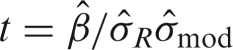 , where
  is the parameter estimate (effect size) for the regressor of interest.
We start with the most simple model, using a boxcar regressor which has a value of 1/2 when there is a stimulus and −1/2 when there is no stimulus. Panel B of Figure 3 shows how poorly this model fits. The small value of and the large residual standard deviation, , result in a test statistic of t = 3.55. This model produces a poor fit, since it assumes that when there is a stimulus the fMRI signal instantaneously increases and then drops as soon as the stimulus ends. In reality, since the fMRI signal is a measurement of hemodynamic change, there is a delay and the response to an event and the model must reflect this. The single gamma (Lange and Zeger, 1997) and double gamma (Glover, 1999) functions are two examples of HRFs.
In order to incorporate the shape of the HRF into our model we convolve the original boxcar regressor with the default HRF from the Statistical Parametric Mapping (SPM) package, the double gamma HRF. Panel C of Figure 3 illustrates how the shape of the regressor more closely fits the shape of the response, which improves the fit of our model to the data causing a decrease in the yellow area between the curves, analogously the residual variance. Notice that the increase in the estimated mean and the decrease in the residual variance contribute to an increase in the test statistic. The variance from the model does not have a noticeable change. Importantly, when using a canonical HRF it is assumed to be correct and if it isn't this could lead to a poorly fitting model. Luo and Nichols (2003) illustrate how the SPM diagnostics toolbox can be used to detect a poorly fitting HRF and Lundquist and Wager (2006) compare methods for estimating the shape of the HRF as well as introducing a new method for HRF modeling.
Now we will focus on the noise of the time series, starting with the low frequency drift which appears in this time series as a downward trend over time. The highpass filter is designed to reduce this type of noise by passing the high frequency noise and reducing the low frequency noise. Software packages handle this issue different ways. The FMRIB Software Library (FSL) fits a weighted running line smoother through the data, which will capture the low frequency trends in the data, and then removes the trend by subtracting the fitted time series from the original time series. The SPM package adds a set of low frequency cosine functions to the design matrix to model the trend. Panel D of Figure 3 shows how the fit of our model is improved by using the cosine basis functions from SPM. Notice how this fitted model curves up at the beginning of the time series fitting the low-frequency drift. The parameter estimate changes only slightly, so the increase in the test statistic is attributed to the decrease in the residual variance. When using a highpass filter you must specify the highest frequency to be filtered from the time series. To avoid filtering out your signal, it is important to choose a limit that is at least as large as twice the stimulation period. So if there were 15 s stimulus blocks followed by 15 s of rest, the highpass filter should be at least 60 s (max frequency=1/60=0.0167Hz) to avoid filtering out the signal.
The lowpass filter filters out high frequency noise. Although this type of filter was used in the past (Friston et al., 2000), it can often interfere with the signal frequency, especially in event-related study designs. Currently highpass filters are rarely used.
Some sources of colored noise, such as cardiac and respiratory function and head motion can be measured. In this case, these noise components can be modeled as fixed effects. These are typically referred to as nuisance variables since there is no interest in carrying out inferences on these variables, but the variables adjust the inferences of the covariates of interest.
The last component to add is a temporal autocorrelation model, which addresses colored noise. When the temporal autocorrelation is ignored, the standard errors from the model will be biased. In the case of positively correlated fMRI time series, the bias produces variance estimates that are too small and hence P-values that are too small, causing false positives. Once the temporal autocorrelation is estimated, the estimate is used to remove the temporal autocorrelation from both the data and the model, a step often referred to as ‘whitening’ or de-noising the model. The correlation model differs between software packages with differences such as the number of parameters used to estimate the correlation and whether the correlation estimate is unique for each voxel or a global estimate. FSL uses a voxelwise unstructured correlation estimate regularized by a Tukey taper then the correlation estimates are spatially smoothed using a nonlinear spatial filter (Woolrich et al., 2001). SPM uses a global correlation estimate of a two-term Taylor series approximation of an autoregressive model [AR(1)] (Friston et al., 2002b). The results in the fifth panel of Figure 3 show the whitened time series and fit of the whitened model, based on the global SPM correlation estimate. The fit of the whitened model does not seem much different than the previous model, but the effect of modeling the autocorrelation is seen by comparing the t-statistics, which are 8.65 and 10.26 for the models with and without an autocorrelation model, respectively. The smaller t-statistic is a result of a slightly larger variance since the positive correlation is now incorporated into the model. Although there may be more significant voxels when not modeling the temporal autocorrelation, due to larger test statistics, many of these will be false positives.
Level 2
For the student opinion change example, the second level models the three estimated university means from the first level assuming each mean has a variance that is a sum of the previously estimated first level variance and a between-university variance. This is similar to a one-sample t-test, but the variance has two parts. In the case of fMRI data we combine the first level signal change parameters and within-subject variances to estimate between-subject variability and carry out inference on group signal change. The signal change parameter estimates from the Level 1 analysis comprise the dependent variable; assume only a single parameter estimate per subject is used. Any group model can then be used, perhaps a single group mean, or the estimation and comparison of two group means. Since we are using a mixed models approach, there are two sources of variability, the within-subject variability, which was estimated in the Level 1 model, as well as a between-subject variability, which is estimated in this level. Specifically, in the group model, subject k has parameter estimate  with variance
 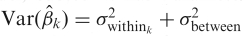 , which is estimated by
 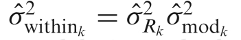 and
and 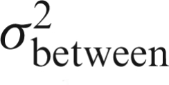 is estimated in the Level 2 model. Once the between-subject variance is estimated, weighted least squares is used to estimate the group model parameters. This is a similar to whitening but instead of temporal autocorrelation there is heteroscedastic variability across subjects.
The estimation of the between-subject variance is carried out in a variety of ways depending on the software used. FSL uses a Bayesian approach and specific details about the model estimation can be found in Beckmann et al. (2003) and Woolrich et al. (2004). SPM, on the other hand, assumes all first level within-subject variances are equal, as a result the within-subject variance is absorbed into the between-subject variance in the Level 2 model. In the case of a single group mean, second level SPM model is equivalent to a one-sample t-test using the N first-level parameter estimated . More details about the SPM model can be found in Friston et al. (2002a) and Friston et al. (2002b).
Specific group fMRI modeling assumptions of different software packages and how they differ are discussed in Mumford and Nichols (2006).
DISCUSSION
When making inference on group fMRI data, it is important to use a mixed model approach to account for both within- and between-subject variability. If a mixed effects model is not used to analyze fMRI data, the results are only applicable to the subjects who participated in the study, not the entire population from which they were sampled. If a fixed effects model is used there will be an increase in false positive test results. Since fMRI data consist of over 100 000 time series that can each be at least 100 time points long, data are analyzed in a voxelwise fashion and the mixed model is broken into two stages, where single subjects are analyzed at the first level and group analyses are carried out at the second level. First level modeling options, including convolution of regressors with HRFs, highpass filtering and correlation estimates, improve the fit of the model and validity of the statistical results. HRF convolution and highpass filtering tend to improve the fit of the model, lowering the residual variance. Modeling the positive correlation of fMRI data reduces bias in the variance estimates, which can cause false positive test results.
Another important issue, not discussed here, is multiple testing of correlated test statistics. Different methods for handling this issue are reviewed by Nichols and Hayasaka (2003).
Acknowledgments
This work was supported by a 21st Century Science Award from the James S. McDonnell Foundation to R.P. Thanks to Joe Devlin and Tor Wager for comments on the manuscript.
Footnotes
Conflict of Interest
None declared.
REFERENCES
- Beckmann CF, Jenkinson M, Smith SM. General multilevel linear modeling for group analysis in FMRI. Neuroimage. 2003;20(2):1052–63. doi: 10.1016/S1053-8119(03)00435-X. [DOI] [PubMed] [Google Scholar]
- Dehaene-Lambertz G, Dehaene S, Anton J-L, et al. Functional segregation of cortical language areas by sentence repetition. Hum. Brain Mapping. 2006;27(5):360–71. doi: 10.1002/hbm.20250. [DOI] [PMC free article] [PubMed] [Google Scholar]
- Friston KJ, Glaser DE, Henson RNA, Kiebel S, Phillips C, Ashburner J. Classical and Bayesian inference in neuroimaging: applications. Neuroimage. 2002b;16(2):484–512. doi: 10.1006/nimg.2002.1091. [DOI] [PubMed] [Google Scholar]
- Friston KJ, Josephs O, Zarahn E, Holmes AP, Rouquette S, Poline J. To smooth or not to smooth? Bias and efficiency in fMRI time-series analysis. Neuroimage. 2000;12(2):196–208. doi: 10.1006/nimg.2000.0609. [DOI] [PubMed] [Google Scholar]
- Friston KJ, Penny W, Phillips C, Kiebel S, Hinton G, Ashburner J. Classical and Bayesian inference in neuroimaging: theory. Neuroimage. 2002a;16(2):465–83. doi: 10.1006/nimg.2002.1090. [DOI] [PubMed] [Google Scholar]
- Glover GH. Deconvolution of impulse response in event-related bold fmri. NeuroImage. 1999;9:416–29. doi: 10.1006/nimg.1998.0419. [DOI] [PubMed] [Google Scholar]
- Holmes A, Friston K. Generalisability, random effects and population inference. Neuroimage. 1998;7:S754. [Google Scholar]
- Lange N, Zeger S. Non-linear Fourier time series analysis for human brain mapping by functional magnetic resonance imaging. Applied. Statistics. 1997;46:1–29. [Google Scholar]
- Lundquist M, Wager T. Validity and power in hemodynamic response modeling: a comparison study and a new approach. Human Brain Mapping. 2006 doi: 10.1002/hbm.20310. [Epub ahead of print] [DOI] [PMC free article] [PubMed] [Google Scholar]
- Luo W-L, Nichols TE. Diagnosis and exploration of massively univariate neuroimaging models. Neuroimage. 2003;19(3):1014–32. doi: 10.1016/s1053-8119(03)00149-6. [DOI] [PubMed] [Google Scholar]
- Mumford J, Nichols T. Modeling and inference of multisubject fMRI data: using mixed-effects analysis for joint analysis. IEEE Engineering in Medicine and Biology Magazine. 2006;25(2):42–51. doi: 10.1109/memb.2006.1607668. [DOI] [PubMed] [Google Scholar]
- Nichols TE, Hayasaka S. Controlling the familywise error rate in functional neuroimaging: a comparative review. Statistical Methods in Medical Research. 2003;12(5):419–46. doi: 10.1191/0962280203sm341ra. [DOI] [PubMed] [Google Scholar]
- Verbeke G, Molenberghs G. Linear Mixed Models for Longitudinal Data. New York: Springer Verlag; 2000. [Google Scholar]
- Woolrich MW, Behrens TEJ, Beckmann CF, Jenkinson M, Smith SM. Multilevel linear modelling for FMRI group analysis using Bayesian inference. Neuroimage. 2004;21(4):1732–47. doi: 10.1016/j.neuroimage.2003.12.023. [DOI] [PubMed] [Google Scholar]
- Woolrich MW, Ripley BD, Brady M, Smith SM. Temporal autocorrelation in univariate linear modeling of FMRI data. Neuroimage. 2001;14(6):1370–86. doi: 10.1006/nimg.2001.0931. [DOI] [PubMed] [Google Scholar]