Combining p-values in large scale genomics experiments

Summary

In large-scale genomics experiments involving thousands of statistical tests, such as association scans and microarray expression experiments, a key question is: Which of the L tests represent true associations (TAs)? The traditional way to control false findings is via individual adjustments. In the presence of multiple TAs, p-value combination methods offer certain advantages. Both Fisher’s and Lancaster’s combination methods use an inverse gamma transformation. We identify the relation of the shape parameter of that distribution to the implicit threshold value; p-values below that threshold are favored by the inverse gamma method (GM). We explore this feature to improve power over Fisher’s method when L is large and the number of TAs is moderate. However, the improvement in power provided by combination methods is at the expense of a weaker claim made upon rejection of the null hypothesis – that there are some TAs among the L tests. Thus, GM remains a global test. To allow a stronger claim about a subset of p-values that is smaller than L, we investigate two methods with an explicit truncation: the rank truncated product method (RTP) that combines the first K ordered p-values, and the truncated product method (TPM) that combines p-values that are smaller than a specified threshold. We conclude that TPM allows claims to be made about subsets of p-values, while the claim of the RTP is, like GM, more appropriately about all L tests. GM gives somewhat higher power than TPM, RTP, Fisher, and Simes methods across a range of simulations.

Introduction

We consider a problem encountered in large scale experiments such as genome-wide association scans. An experiment like this is usually preliminary in the sense that the primary goal is to identify a set of promising genetic variants, possibly predictive of a trait such as a disease. Results of the experiment are typically ordered by a measure of association such as a p-value, and a certain number of best-ranking results become candidates for a follow-up study. A follow-up study may consist of efforts to replicate the putative associations in independent samples, and additional genetic markers can be typed in the vicinity of the original associations. It is generally understood that the TAs may be only loosely clumped among the best-ranking results, and some may not be captured at all. Thus, statistical methods that allow making simultaneous claims about sets of results are important. A recent comprehensive overview of association scans, their goals, design and interpretation of results, including multiple testing issues is given in Hirschhorn and Daly [1].

Zaykin and Zhivotovsky [2] investigated the problem of TA ranks by examining the distribution of their relative position among the results ordered by a measure of association. They considered multiple effects including situations with highly correlated test statistics. The correlation in those experiments was due to linkage disequilibrium (LD) between alleles of neighboring genetic polymorphisms. Neither monotone decay nor block-structured LD was found to affect the distribution of ranks to a substantial degree. This is due to the local nature of LD that drives the correlation in association studies, in contrast to the recombination-driven correlation in linkage studies, which extends throughout large chromosomal segments. In the presence of multiple TAs, two questions regarding the ranks can be asked: (1) what is the distribution of the rank associated with the best-ranking TA – this is an issue of finding at least one of the multiple TAs; and (2) what is the distribution of the rank of the worst-ranking TA, which is an issue of finding all of the multiple TAs. These questions are related to the distribution of the first and the last order statistics associated with the TAs. In the first case, the ranks are improved, subject to the argument that in the context of genetically determined traits, magnitudes of each of the effects tend to decrease, as the number of effects increases. While each individual effect and the associated power might be small, discovery and the ability to score weakly predictive variants can be utilized to create highly predictive profiles involving multiple effects.

Regarding the practical issue of detecting multiple TAs, methods that combine p-values are especially promising. Many common methods for combining p-values are of the following form. First, take a transformation H of p-values, T_i = H (p_i); next, evaluate $Y={\sum }_{i=1}^L{T}_i$, where L is the total number of tests. Y is a combined test statistic, with cumulative distribution function (CDF) denoted by F (·). The combined p-value is p^c =1−F(Y). Zaykin et al. [3] discussed several such methods. Stouffer’s method takes H to be the inverse standard normal CDF, which results in F being a normal distribution. Edington’s method simply takes the sum of p-values and evaluates the CDF of the resulting random variable. The Fisher combined probability (FCP) method takes H (p_i) = −2ln( p_i), which results in F being a chi-square with 2L degrees of freedom. Note that the combined p^c in FCP can be obtained by taking the product of p-values, W, and evaluating its distribution, because Pr(Π p_i <w)= Pr(Σ − 2ln(p_i) < −2ln(w)). The binomial (Wilkinson’s) test counts the number of p-values that are below a threshold τ (where τ could be taken to be the nominal significance level, α). It has the transformation $H(p_i)={\sum }_{i=1}^{L}I(p_i\le \tau )$, so that F is the binomial CDF.

In research published before modern computing power was prominent, the form of H was typically dictated by the ease with which the resulting distribution F could be evaluated. Nowadays any form of H can be used with the aid of a simple Monte Carlo evaluation: (1) Calculate T₀ = ΣH(p_i), using the observed set of p-values. (2) Generate T_j = ΣH (p_i) for j=1,…,B simulations, where p_i ~ Uniform(0,1). The proportion of T_j ≤ T₀ gives the combined p-value, p^c. Zaykin et al. [3], Dudbridge and Koeleman [4], and Lin [5] extended this basic approach by considering ways to allow for dependencies among p-values.

Truncated Product and Rank Truncation Product Methods

For any choice of transformation H, combined p-value statisticscan also be computed on subsets of all L p-values. The truncated product method (TPM) of Zaykin et al. [3] uses only p-values that are below some threshold τ. Significance is assessed by evaluating the distribution of their product, thus the method brings together the features of Fisher’s and the binomial methods. In contrast, the rank truncation product method (RTP; [6], [7], [8]) takes the product of the first K p -values and evaluates its distribution. When K=L, this method reduces to Fisher’s method.

The choice of the transformation H is highly relevant in our context of extreme heterogeneity among effects, where only a proportion of them might be non-zero. Methods such as TPM or RTP specify an explicit threshold such that large p-values above the threshold are penalized. When the TPM threshold τ is equal to the minimum p-value, p₍₁₎, or when K=1 in the RTP method, both of the methods reduce to the Śidák correction, 1− (1 − p₍₁₎)^L (keeping in mind that with the exception of p₍₁₎, the value of τ cannot be chosen based on an observed p-value, and should be specified in advance).

Soft Truncation Threshold

Even without an explicit truncation, any form of H implicitly imposes what we call the “soft truncation threshold” (STT), a feature important in situations when there is pronounced heterogeneity of effects. Consider Fisher’s method as an example. Elston [9] noted that in the limit (L → ∞) Fisher’s method favors p-values that are below 1/e ≈ 0.368. That is, if all p-values are equal to 1/e, the combined p^c is also 1/e. If all p-values are smaller than 1/e, the combined p^c goes to zero, and if they are larger that 1/e, the p^c goes to one. Thus, 1/e provides a threshold point for Fisher’s method, which we call the STT value. Compare this to the inverse normal (Stouffer’s) method, where the threshold is 0.5 – the expected value of a p-value under the null hypothesis (H₀). Rice [10] argued that methods like Stouffer’s are more appropriate for the situation when all L tests address the same null hypothesis, for example during meta-analysis, so that p^c has an interpretation as a “consensus p-value”. It is expected that Fisher’s method should have a higher power to reject the overall (i.e. intersection) hypothesis under effect heterogeneity, as was found in simulations in [3]. In the most extreme case, when there is always only a single TA among the L tests, adjusted p-value methods such as the Śidák correction are more powerful than any of the combination methods.

The threshold of Fisher’s method is somewhat smaller than 1/e for any finite value of L. The example of L=2 is illustrative. In this case, Fisher’s combined p-value can be found as $p^c=1-{\displaystyle \underset{w}{\overset{1}{\int }}}{\displaystyle \underset{t}{\overset{1}{\int }}}(1/v)\hspace{0.17em}dvdt=w[1-ln(w)]$, where w is the product of the two p-values. Thus, the STT for L=2 can be found by determining the value of p such that p² [1 − ln(p²)] = p. This value is 0.284668 < 1/e. For larger values of L, it is convenient to take the log of the product and find the value numerically by solving 1− F[L, 1; − L ln(x)] = x, where F denotes the Gamma(L, 1) CDF evaluated at − Lln(x). For example, with L=100, the STT is ≈ 0.356; thus, the value is approaching 1/e. A notable feature of this threshold is its invariance in the presence of correlations between p-values. First, we note that under the independence of p-values, the value 1/e can be found by a Central Limit Theorem argument, as the solution for x in $1-\mathrm{\Phi }[\sqrt{L}(-ln(x)-1)]=1/2$, where Φ (·) is the standard normal CDF. Assume the correlations are of the kind as to give convergence of Y = −Σ ln( p_i) to the normal distribution for correlated p-values. The presence of correlations has an effect of increasing the variance of Y. However, the solution of 1−Φ [C (−ln(x) −1)] =1/2 is x = 1/e for any constant C, therefore the limit threshold remains the same as in the independence case.

Gamma Method

Fisher’s method is in essence to add up a series of two-degree-of-freedom chi-squares; however, the degrees of freedom do not need to be the same. An explicit weighting of p-values was given by Good [11]. Lancaster [12] suggested that varying degrees of freedom can be used to weight the respective p-values and proposed a weighted modification where the degrees of freedom can be taken to be equal to the sample sizes of the combined experiments. In Lancaster’s method, $Y={\displaystyle \sum _{i=1}^L}{G}_{d_i/2,2}^{-1}(1-p_i)$, where the transformation H is $G_{d_i/2,2}^{-1}(1-p_i)$, the inverse of the Gamma(d_i/2,2) CDF, which is the chi-square CDF with d_i degrees of freedom. Thus, under H₀, Y has a chi-square distribution with Σd_i degrees of freedom.

The following modification (which we call the “Gamma Method”, GM) exploits the same feature of the Gamma distribution as Lancaster’s weighting method - that a sum of gamma-distributed random variables with the same rate still has a gamma distribution. The rate does not affect the combined p^c, and we will assume the rate to be 1. Let the transformation H be $G_{a,1}^{-1}(1-x)$, the inverse of the Gamma(a, 1) CDF. The combination method GM is defined by

$$\begin{array}{l}Y=\sum _{i=1}^L{G}_{a,1}^{-1}(1-p_i)\\ p^c=1-G_{La,1}(Y)\end{array}$$

Thus, the method utilizes the common shape value (a) for the gamma distribution. A specific value is chosen to explicitly control the STT. When a is large, the gamma CDF becomes the normal inverse method, which has an STT of 0.5. The procedure becomes Fisher’s method when a=1, with the STT as discussed above. For a given STT=x, the large L value of a can be found by solving $a=G_{a,1}^{-1}(1-x)$. For example, a=0.0137 gives STT=0.05; a=0.0383 gives STT=0.1; and a=1 gives STT=1/e. The finite L values of a for a given value of STT=x are found by solving $x=1-G_{La,1}\left(L{G}_{a,1}^{-1}[1-x]\right)$. For STT=0.05 with L=10, the value of a is 0.0346.

Simulation Results

Table 1 gives results of a power evaluation in experiments with L=5000 and using one-degree-of-freedom chi-square tests. The number of TAs ranges from 10 to 200 with various powers specified for the individual effects at the level of 5%. The number of simulations to obtain a set of power values for each row was at least 10000. The STT values of 0.05 and 0.10 for the GM in the table are for infinite L. It appears from these experiments that GM with a low STT provides good overall power across different combinations of parameters. The method is most successful in situations with relatively low proportions of TAs when there is still advantage in using combination tests over family-wise error rate (FWER) adjustments such as the Śidák correction. We found that values of STT lower than 0.05 created difficulties with the numerical evaluation of the Gamma distribution by the DCDFLIB routines [13], possibly because the distribution becomes concentrated at zero when the parameter a is too small. In these cases, we observed somewhat inflated type-I error rates. The chosen values (STT of 0.05 and 0.10), or values higher than that were verified to give a correct proportion of rejections under H₀, i.e. when the number of TAs=0.

Table 1.

Simulation Results Comparing Power of Different Combined P-Value Methods

Śidák	Simes	GM (0.05)	GM (0.1)	TPM (0.05)	TPM (0.01)	TPM (0.005)	TPM (0.001)	RTP (10)	RTP (50)	RTP (100)	RTP (200)	FCP
#TA: 10; Power: 90%
0.738	0.756	0.791	0.650	0.279	0.455	0.550	0.752	0.879	0.814	0.739	0.625	0.225
#TA: 50; Power: 50%
0.335	0.351	0.799	0.789	0.595	0.650	0.656	0.601	0.636	0.751	0.769	0.764	0.525
#TA: 50; Power: 60%
0.529	0.553	0.961	0.950	0.788	0.876	0.888	0.864	0.875	0.947	0.951	0.942	0.693
#TA: 100; Power: 30%
0.178	0.181	0.644	0.697	0.595	0.543	0.495	0.378	0.377	0.544	0.607	0.649	0.598
#TA: 100; Power: 40%
0.327	0.339	0.926	0.944	0.861	0.853	0.825	0.715	0.703	0.874	0.907	0.926	0.831
#TA: 200; Power: 20%
0.138	0.143	0.653	0.746	0.696	0.563	0.490	0.332	0.314	0.511	0.605	0.682	0.756
#TA: 200; Power: 25%
0.203	0.216	0.883	0.936	0.895	0.814	0.742	0.545	0.509	0.765	0.847	0.904	0.920
#TA: 200; Power: 30%
0.290	0.300	0.978	0.992	0.980	0.949	0.915	0.764	0.715	0.932	0.967	0.984	0.981

The overall power of GM for the chosen combinations of power for individual TAs and the numbers of TA is consistently higher than the power of other methods. However, there is arbitrariness in the choice of parameters of the three methods. For example, it is possible to increase power for all three methods in the settings with the number of TAs=200, by increasing K, τ, and the STT. A more expanded set of these values was applied to the setting with the number of TAs=200 at 20% power. Note that for this setting, the best test in Table 1 is FCP. By examining a wide range of parameters, we found that GM at STT=0.25 gave the best power (0.800) among all methods;. TPM power kept increasing up to τ=1 (0.756 power); and the best value of K for the RTP was found to be K=1300 (0.786 power). The increments used were 0.05 for STT and τ, and 100 for K. Next, we repeated this experiment for the setting with TAs=200 at 25% power. For GM the maximum power was 0.954 at STT=0.2; for TPM, the maximum power was 0.908 at τ=0.15; for RTP the maximum power was 0.945 at K=1300. Thus, in both extended cases the GM provided a higher power, and the difference is highly statistically significant by the Mann-Whitney test.

Although the power of RTP is very close to that of the GM, there appears to be a greater uncertainty about the choice of the parameter K. When the power is low, the best value of K tends to be much higher (we will discuss this phenomenon in more detail below). On the other hand, the best choice of the STT parameter for GM appears to be around 0.25 when the number of TAs is equal to 200. It is still affected by the proportion of TAs to false associations (FAs), but not so much by the power associated with the TAs. To illustrate this, Figure 1 shows combination test power values for the GM when the individual power varies from 10% (lower graph) to 30% (upper graph). The best STT value is between 0.20 (for 30% power) and 0.30 (for 10% power). Note that because both Fisher’s and the inverse normal (Stouffer’s) methods are particular cases of the GM, the X axis in Figure 1 includes Fisher’s method at X = 1/e and the inverse normal method at STT = 0.5.

Figure 1. Power of the Gamma combination method at different values of the STT with 200 TAs and 4800 FAs.

The lowest curve (with open circle points) corresponds to 10% power for the individual TAs. The curves above that are at 15%, 20%, 25%, and 30% power, correspondingly.

The Simes test [14] has been included in Table 1 for comparison. There are certain advantages in using this test, for example, it is robust in the presence of correlations [15]. However, a feature of this test is that the overall p-value cannot be smaller than the minimum p-value, p₍₁₎, while methods that combine p-values explicitly can give an overall p that is smaller than p₍₁₎. In our case of relatively small power to detect the individual TAs, this yields a higher overall power.

Difference in Interpretation of TPM and RTP Rejections

Although the simulation results for GM in Table 1 appear very promising, we focus attention for the remainder of this report on TPM and RTP in order to address some fundamental issues of interpretation. In Table 1 and the extended results described previously, RTP exhibits higher power than TPM. However, there are important differences in the way the null hypothesis of RTP and TPM are formulated, and the claims one can make upon the rejection of the null. The claim of the TPM is that upon rejection of the null, there are one or more TAs among the effects represented by p-values that are at least as small as the truncation threshold, τ. We are careful not to assign a degree of certainty or probability to this event, and still give the corresponding p-value a standard frequentist interpretation. On the other hand, one cannot make a similar claim with the RTP: i.e. that there is at least one TA among the effects represented by the first K p-values.

An intuitive explanation for this phenomenon is as follows. The requirement that the TA p-values should rank above K would be satisfied more often when the FA p-values happened to be unusually small. Thus, if we evaluate the proportion of rejections among experiments where all TAs rank above the K, we would expect it to be above the nominal level. However, there is no similar dependency among the TAs and the FAs for the TPM with any truncation threshold τ – the event that all TA p-values are larger than τ simply has an effect of increasing L without affecting the value of the p-value product.

To verify these assertions, we conducted the following additional simulations. To evaluate RTP under the above scenario, we generated 5 true effects for each simulation experiment with L=25 and individual power 70% for a TA, under the condition that the first 5 smallest p-values represent FAs. We rejected simulated samples where this was not the case. Next, we took the product of the first K=5 p-values and obtained the computed p^c. In these simulations, RTP still had 30% power to reject the hypothesis that there are no true effects among the total of L hypotheses. Taking a smaller value of K=3 still gave 21% power. The power increased to 47% for K=10. An analogous simulation for the TPM involved L=100, and 10 TAs with 99% power each. In these simulations, experiments with the TA p-values stronger than 0.05 were rejected. As expected, the proportion of rejections for the TPM with τ=0.05 was conservative: 2.9% at the level α=5% and 6.5% at α=10%. However, TPM gained power when the truncation threshold was increased. The power was 29% and 37% for τ =0.1 and τ=0.2, correspondingly (at α=5%).

It is possible to modify TPM for interpretation on a narrower rejection set, and Appendix 1 describes details of one possible approach. This is reminiscent of an issue with Benjamini and Hochberg’s [16] false discovery rate (FDR) where FDR = E[F/(T+F) | T+F > 0] Pr(T+F > 0), denoting True and False discoveries by T and F. The difference with TPM is that we don’t necessarily know what Pr(T+F > 0) is, and in fact this probability can decrease to α as L increases. This would happen in settings such as association genome-wide scans, where most added hypotheses are FAs, so that the prior proportion of TAs would approach zero. In this case, E[F/(T+F) | T+F > 0] approaches 1, and Pr(T+F > 0) approaches α. Then across the sets of L experiments, FDR rejects α% of the time, as it should, because it becomes the Simes test which is known to maintain “weak control” of the FWER. The value of Pr(T+F > 0) depends on power and also on the prior Pr(H₀) (in other words, on the population proportion of FAs). Thus, we cannot easily obtain the FDR conditional on having made rejections, E[F/(T+F) | T+F > 0], which would be interpreted as the “proportion of false rejections among rejections”. Nevertheless, in certain settings such as microarray expression experiments, where the proportion of TAs is large and does not decrease with L, Pr(T+F > 0) may approach 1 and the conditional interpretation of FDR is warranted.

Care must also be taken in interpreting the value of K used with RTP. Closely related to RTP is the Set Association Method by Hoh et al. [17] proposed for large-scale genome association experiments. The set association approach is to take the sum of the first K largest association test statistics, $S_K={\sum }_{i=1}^k{T}_i$, to form an overall test that includes the K most significant genetic markers. Hoh et al. proposed finding the value of K that maximizes the significance of S_i, obtained from its Monte Carlo permutation distribution. While the method results in a powerful test under models with multiple contributing factors, there is a temptation to interpret the value of K that corresponds to the minimum permutational p-value for the combined test statistic (S_K) as being an estimate of the number of true associations. For example, in studying association of glucocorticoid-related genes with Alzheimer’s disease, de Quervain et al. [18] interpret the optimal value of K as an estimate of the number of TAs and write that the additional markers “indicate SNPs not contributing to the disease risk significantly, i.e. p-value is increasing due to introduction of statistical noise”. However, such an estimate is biased, for the reason that true associations tend to spread over a number of individual test results that are ordered by significance. When m is much smaller than L, and the power corresponding to TAs is low, then TAs tend to be interspersed with the first order statistics of FAs. Up to a certain value of i, these first order statistics (X_i) will have p-value distributions which are more skewed toward zero compared to those of TAs, given that the value of L is sufficiently large. Therefore the set association method is likely to reach its highest power for values of K > m. If individual test statistics are independent and follow a chi-square distribution, finding the p-value associated with S_k is equivalent to computing Pr(W_K ≤ w), where $W_K={\prod }_{i=1}^K{P}_i$, w is the observed value for the product, and P_i are ordered random p-values corresponding to individual association tests. Thus, the method is equivalent to the RTP method discussed above. Appendix 2 provides an analytical derivation of the product distribution and further theoretical justification for the preceding bias claims.

Discussion

In situations with multiple TAs that are a small proportion relative to the overall number of tests, L, truncation p-value combination methods become more powerful, although the claims associated with these methods are less specific. The objective of these approaches is to combine a subset of promising p-values, while taking into account all L tests. Focusing on a subset of small p-values can be achieved by combining the K smallest p-values such as in RTP, or by combining p-values that are smaller than a threshold τ, as in TPM. While RTP is often able to provide higher power than TPM (at τ < 1), TPM allows one to make stronger claims. In the event of rejection, the TPM claim is that there are genuine effects among those represented by p-values that are smaller than τ. The RTP claim remains the same as that of Fisher’s combination test: that there are genuine effects among all L tests. This is less specific than the claim of TPM, despite the fact that a certain value K<L led to a rejection.

The RTP and TPM formulations involve an explicit threshold, the p-value rank or the p-value magnitude, respectively. An alternative method based on the inverse gamma transformation (GM) was found to provide an overall combination test that was more powerful in simulations. A parameter of this method allows a control of what we call the soft truncation threshold (STT) – the value that favors p-values that are smaller than the STT. GM provides high power at fixed values of the STT across settings where both the power and the number of TAs are allowed to vary. In principle, it is possible to bring together the advantages of the TPM and the GM. Such a method would consider a sum of transformed p-values among p-values that are smaller than a specified threshold.

Adjustments for individual p-values can be based on any of the combination methods via the closure principle [19]. A computational shortcut is available for TPM as described in Appendix 2 of Zaykin et al. [3]. The same closure shortcut is applied for GM for p-values as small as the STT.

Appendix 1 Modified TPM

We here describe a TPM modification, where the H₀ rejection claim pertains to the subset of experiments where at least one p-value is ≤ τ. At the value of L=100, such as in the above simulations, the probability of at least one p-value falling below τ=0.05 is 99.4%, which is almost a certainty. In general, however, the standard TPM claim is that the probability of rejection under H₀ is α, including experiments where p₍₁₎ > τ. In the case when p₍₁₎ >τ, H₀ is accepted, and then the overall rate of rejections across all experiments, including these, is α. However, it is easy to make a modification so that in the case of the H₀ rejection, the claim excludes subsets of experiments with p₍₁₎ > τ, which under the H₀ happens with probability 1− (1−τ)^L. Denote the product of all p-values less than the truncation τ by W, and its observed value by w. The TPM combined p-value = Pr(W ≤ w) under H₀. Zaykin et al. [3] obtained the following formula for independent p-values:

$$\begin{array}{l}Pr(W\le w)=\sum _{k=1}^L\left(\begin{array}{c}L\\ k\end{array}\right){(1-\tau )}^{L-k}\\ \times \left(w\sum _{s=0}^{k-1}\frac{{(kln\tau -lnw)}^s}{s!}I(w\le {\tau }^k)+{\tau }^{k}I(w>{\tau }^k)\right)\end{array}$$

where I (·) is the indicator function. For τ =1, this formula gives Fisher’s combined p-value: $Pr(W\le w\mid \tau =1)=w{\displaystyle \sum _{s=0}^{L-1}}\frac{{(-lnw)}^s}{s!}$. The value of Pr(W ≤ w) cannot exceed 1− (1−τ)^L, and is equal to it when p₍₁₎ = τ. This p-value is

$$\begin{array}{l}Pr(W\le w)=Pr(W<w\mid p_{(1)}<\tau )Pr(p_{(1)}<\tau )\\ =Pr(W<w\mid p_{(1)}<\tau )\left(1-{[1-\tau ]}^L\right)\end{array}$$

Therefore, the TPM p-value concerning the subsets with at least one p-value ≤ τ is

$$p^{\ast }=\frac{Pr(W<w)}{1-{(1-\tau )}^L}$$

As an example, suppose the TPM p-value is 0.01, τ=0.05, and L=25. Then p* = 0.014, which is larger than 0.01. However, the modification gives a stronger interpretation: p* is the combined probability under the null for the subset of experiments where at least one p-value is less than τ.

Appendix 2 Distribution of W_K for RTP

Given the ordered set of random p-values, {P₁, P₂,…, P_L}, it is possible to obtain the distribution of the product of the first K smallest p-values under the null hypothesis (m=0). Dudbridge and Koeleman [6] give such expression, derived by conditioning on P_K+1. Although this is undefined for k=L, some simple adjustments can be made to get around this case; for example a random variable can be defined as X=P_K+1 for K<L and X=1 for the case K=L, and then the conditioning is made on X (Dudbridge, personal communication).

Now we will give an alternative form of the distribution that covers all cases. The distribution of the K-th smallest p-value itself is P_K ~ Beta(K, L−K+1). The product of the first K smallest p-values, W_K, can be written as

$$\begin{array}{l}{W}_K=\left(\frac{P_1}{P_2}\right){\left(\frac{P_2}{P_3}\right)}^2\dots {\left(\frac{P_{k-1}}{P_k}\right)}^{K-1}\\ U_i=P_{i-1}/P_i\\ P_K^K=U_1{U}_2^2\dots U_{K-1}^{K-1}{P}_K\end{array}$$

The variables $U_1,U_2^2,\dots ,U_{K-1}^{K-1},U_K$ are independent with distributions

$$\begin{array}{l}{U}_i\sim \text{Beta}(i,1)\\ U_i^i\sim \text{Uniform}(0,1)\end{array}$$

The variable $P_K^K$ is the K-th power of the Beta(K, L−K+1) random variable with the density $P_K^K\sim \left(\begin{array}{c}L\\ K\end{array}\right){(1-x^{1/K})}^{L-K}$. Then the product distribution is

$$\begin{array}{l}Pr(W_K\le w)=1-\underset{w}{\overset{1}{\int }}\left(\begin{array}{c}L\\ K\end{array}\right){(1-x^{1/K})}^{L-K}\\ \times \underset{w}{\overset{1}{\int }}\underset{\frac{w}{x_2}}{\overset{1}{\int }}\underset{\frac{w}{x_2{x}_3}}{\overset{1}{\int }}\dots \underset{\frac{w}{x_2\dots x_{K-1}}}{\overset{1}{\int }}d{x}_1\dots d{x}_K\\ =1-\left(\begin{array}{c}L\\ K\end{array}\right)\underset{w}{\overset{1}{\int }}{(1-x^{1/K})}^{L-K}\\ \times \left[1-\frac{w}{x}\sum _{j=0}^{K-2}\frac{{\left(ln\frac{x}{w}\right)}^j}{j!}\right]dx\end{array}$$

In practice, this integral requires a numerical evaluation. Figure 2 shows a bias resulting from interpreting the value of K that minimizes Pr(W_K ≤ w) in an experiment with m=50 true (with the individual power of 40%) and L−m=5000 false associations. Figure 2(a) shows the power (y-axis) of the test based on Pr(W_K ≤ w), assuming a given value of K on the x-axis. The number of TAs is estimated from the graph to be around 200, corresponding to the value of k that gives the largest power. Figure 2(b) shows the value of K plotted against the expected −ln(p-value), which again gives the maximum at K=200. Interestingly, there is no monotonicity in going from K=1 (Śidák correction) to K=2,3, etc. In a separate experiment with power of individual effects increased to 50%, the maximum was found at K=100. When the power was decreased to 30%, the optimum K was at 500. Thus, with a simultaneous increase in power at each of the true m effects, the “best” K approaches the true value, m. However, the peak tends to be flat, with the estimate of m being imprecise [4]. The decrease in the number of TAs tends to give power advantage to the RTP with K=1 (Śidák) and to other FWER-controlling methods. We suggest that the best interpretation of results from the tests based on the sum of the largest effects (or largest test statistic values) is that there might be an indication of several TAs if the resulting p-value is found to be small. A value of K associated with the most significant S_K should not be regarded as an estimate of the number of TAs. Nevertheless, such tests can be quite powerful and useful as providing evidence against the overall null hypothesis including all L hypotheses.

Figure 2. Simulations with L=5000; number of TA=50 with the individual power 40% at α =5%.

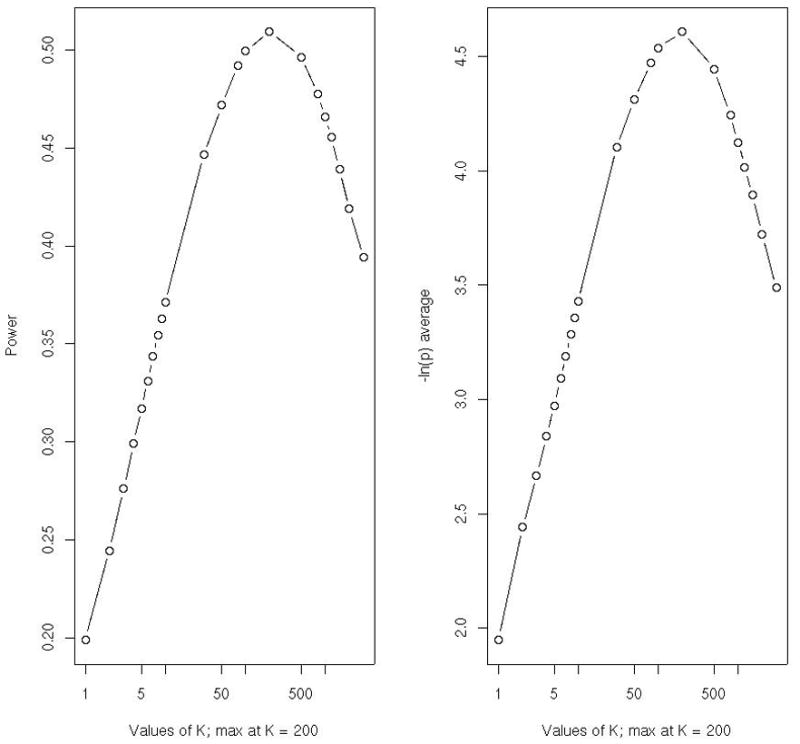
(a) Plot of power of the RTP as a function of K.

(b) Plot of expected −log(p-value) as a function of K.

References

- 1.Hirschhorn JN, Daly MJ. Genome-wide association studies for common diseases and complex traits. Nat Rev Genet. 2005;6:95–108. doi: 10.1038/nrg1521. [DOI] [PubMed] [Google Scholar]
- 2.Zaykin DV, Zhivotovsky LA. Ranks of genuine associations in whole-genome scans. Genetics. 2005;171:813–823. doi: 10.1534/genetics.105.044206. [DOI] [PMC free article] [PubMed] [Google Scholar]
- 3.Zaykin DV, Zhivotovsky LA, Westfall PH, Weir BS. Truncated product method for combining P-values. Genetic Epidemiology. 2002;22:170–185. doi: 10.1002/gepi.0042. [DOI] [PubMed] [Google Scholar]
- 4.Dudbridge F, Koeleman BP. Efficient computation of significance levels for multiple associations in large studies of correlated data, including genomewide association studies. American Journal of Human Genetics. 2004;75:424–435. doi: 10.1086/423738. [DOI] [PMC free article] [PubMed] [Google Scholar]
- 5.Lin DY. An efficient Monte Carlo approach to assessing statistical significance in genomic studies. Bioinformatics. 2005;21:781–787. doi: 10.1093/bioinformatics/bti053. [DOI] [PubMed] [Google Scholar]
- 6.Dudbridge F, Koeleman BP. Rank truncated product of P-values, with application to genomewide association scans. Genetic Epidemiology. 2003;25:360–366. doi: 10.1002/gepi.10264. [DOI] [PubMed] [Google Scholar]
- 7.Zaykin DV, Zhivotovsky LA. Unpublished, 1998.
- 8.Zaykin DV. PhD thesis. North Carolina State University; Raleigh: 1999. Statistical analysis of genetic associations. [Google Scholar]
- 9.Elston RC. On Fisher’s method of combining p-values. Biometrics. 1991;33:339–345. [Google Scholar]
- 10.Rice WR. A consensus combined p-value test and the family-wide significance of component tests. Biometrics. 1990;46:303–308. [Google Scholar]
- 11.Good IJ. On the weighted combination of significance tests. Journal of the Royal Statistical Society (B) 1955;17:264–265. [Google Scholar]
- 12.Lancaster HO. The combination of probabilities: an application of orthonormal functions. Australian Journal of Statistics. 1961;3:20–33. [Google Scholar]
- 13.Brown B, Lovato J, Russell K. Technical report. University of Texas; Houston: 1997. DCDFLIB: library of C routines for cumulative distribution functions, inverses, and other parameters, release 1.1. [Google Scholar]
- 14.Simes RJ. An improved Bonferroni procedure for multiple tests of significance. Biometrika. 1986;73:751–754. [Google Scholar]
- 15.Sarkar S, Chang CK. Simes’ method for multiple hypothesis testing with positively dependent test statistics. Journal of the American Statistical Association. 1997;92:1601–1608. [Google Scholar]
- 16.Benjamini Y, Hochberg Y. Controlling the false discovery rate - a practical and powerful approach to multiple testing. Journal of the Royal Statistical Society (B) 1995;57:289–300. [Google Scholar]
- 17.Hoh J, Wille A, Ott J. Trimming, weighting, and grouping SNPs in human case control association studies. Genome Research. 2001;11:2115–2119. doi: 10.1101/gr.204001. [DOI] [PMC free article] [PubMed] [Google Scholar]
- 18.de Quervain DJ, Poirier R, Wollmer MA, Grimaldi LM, Tsolaki M, Streffer JR, Hock C, Nitsch RM, Mohajeri MH, Papassotiropoulos A. Glucocorticoid-related genetic susceptibility for Alzheimer’s disease. Human Molecular Genetics. 2004;13:47–52. doi: 10.1093/hmg/ddg361. [DOI] [PubMed] [Google Scholar]
- 19.Marcus R, Peritz E, Gabriel KR. On closed testing procedures with special reference to ordered analysis of variance. Biometrika. 1976;63:655–660. [Google Scholar]