Image Reconstruction in SNR Units: A General Method for SNR Measurement

Abstract

The method for phased array image reconstruction of uniform noise images may be used in conjunction with proper image scaling as a means of reconstructing images directly in SNR units. This facilitates accurate and precise SNR measurement on a per pixel basis. This method is applicable to root-sum-of-squares magnitude combining, B₁-weighted combining, and parallel imaging such as SENSE. A procedure for image reconstruction and scaling is presented, and the method for SNR measurement is validated with phantom data. Alternative methods that rely on noise only regions are not appropriate for parallel imaging where the noise level is highly variable across the field-of-view. The purpose of this article is to provide a nuts and bolts procedure for calculating scale factors used for reconstructing images directly in SNR units. The procedure includes scaling for noise equivalent bandwidth of digital receivers, FFTs and associated window functions (raw data filters), and array combining.

Signal-to-noise ratio (SNR) is a frequently used metric of image quality, yet despite numerous proposed methods for measuring SNR in MR images (1–4), a number of important issues remain. In this article, current methods and limitations will be reviewed. A method for reconstructing images directly in SNR units is described. This approach facilitates accurate and precise SNR measurement on a per pixel basis and is applicable to root-sum-of-squares magnitude combining, B₁-weighted combining, and parallel imaging. Alternative methods that rely on measurement of noise from regions of interest in the signal-free background (1,2) are not appropriate for parallel imaging where the noise level is highly variable across the field-of-view. The variation in noise across the FOV, the so-called g-factor (5), arises due to the ill-condition of the inverse solution used in parallel imaging. As parallel imaging (5) is now widely used, a procedure is needed to accurately and precisely measure SNR. The purpose of this article is to provide a nuts and bolts procedure for calculating scale factors used for reconstructing images directly in SNR units. The procedure includes scaling for noise equivalent bandwidth of digital receivers, FFTs and associated window functions (raw data filters), and array combining.

SNR images provide a number of benefits. Protocols may be optimized by quantitative measurement of image SNR as parameters such as TE, TR, bandwidth, and readout flip angle are varied. Comparison between sequences and protocols is easier to perform and more reliable, as well as comparison between various coil designs and coil placement. Clinical benefits include quantitative characterization of lesions and tissue. Questions such as how much lesion enhancement or how much change is observed day-to-day may be answered with greater confidence. Quantitative measurements of contrast-to-noise (CNR) determine if a region has a statistically significant difference in intensity. Variation in tissue intensity due to heterogeneity may be discriminated from variation due to thermal noise. Quantitative measures of SNR and CNR are useful in first-pass contrast enhanced perfusion studies. Post-Processing of images is also facilitated with SNR scaled images, e.g., simple thresholding.

SNR is frequently calculated using noise SD values estimated directly from the reconstructed image or series of images. A number of methods for estimating the noise SD are described briefly in the following. These methods have limitations that serve as a motivation for using SNR scaled image reconstruction, which is based on pre-scan noise measurement. The methods of noise estimation fall into 3 general classes: (a) estimating background noise based on a noise only region; (b) estimating noise based on temporal differencing or, more generally, temporal filtering; and (c) estimating noise based on spatial derivative or highpass filter.

The method of background noise estimation from the noise only region (1,2) is perhaps the most commonly applied method. The user manually selects a noise only region within the field-of-view. The SD may be estimated from pixels in this region. The error in the SD estimate is proportional to 1/√N (6), where N is the sample size (number of independent pixels); therefore, hundreds of pixels are required to obtain reasonable estimates. In the case of magnitude images, the signal and noise values must be corrected (1,2) to calculate SNR due to the fact that magnitude detection alters the probability distribution of noise. The correction depends on the SNR as well as the number of receiver coils. As surface coil arrays with a larger number of elements are used, the noise biases and correction become more significant. While the scaling and correction are straightforward, there still remains confusion on this subject in practice. Measurement of background noise in this manner has a number of drawbacks, which include: difficulty in finding noise only regions within the FOV, limited precision due to small sample size, contamination of noise only region by artifacts, errors due to improper treatment of correlated noise, unsuitability for parallel MR image reconstruction where the noise may be highly variable across the field of view, and need for manual tracing of the noise region.

A second approach to noise estimation is to subtract images in order to cancel the stationary signal, and thereby obtain noise only (3). In this case, an estimate of the noise SD may be obtained in regions of interest that contain signal, provided that the intensity in the desired region is stationary. Differencing may be further generalized to highpass filtering of a time series of consecutive images. In this case, the highpass filter may be designed to suppress a range of temporal fluctuation frequencies. Drawbacks to this approach include the requirement to acquire multiple images; requirement for stationary tissue, which excludes many applications such as cardiac imaging; and limited precision due to small sample size. Furthermore, this method does not distinguish between thermal background noise and physiologic fluctuation, which have different significance depending on the application. This approach does have the benefit of measuring the local noise, limited by the ROI size, which determines precision, and, therefore, may be used for applications such as parallel MR with greater accuracy and precision than the use of the background noise-only approach.

A third approach is to estimate noise after spatial differentiation to eliminate signal in homogeneous regions with highly constant signal intensity (4). This may also be implemented using a generalized spatial highpass filter. This approach may be used with single image acquisitions, but is limited in applicability to relatively large regions with little to no intensity variation. The precision is again determined by the ROI size, which is limited by the size of the structure. Since the noise estimate is local, it may be used with parallel MR with limited accuracy.

The method proposed in this article estimates noise statistics from noise only data (i.e., acquired without RF pulses), which may be automatically acquired by the sequence immediately prior to signal acquisition (referred to as pre-scan noise). Therefore, the precision of estimating noise statistics may be extremely good since a large number (thousands) of samples may be acquired in a relatively short time. Furthermore, the estimates of the noise covariance between channels may be used for optimal array combining to improve SNR, as well as measurement accuracy. Optimum array combining frequently combines channels based on relative rather than absolute noise levels. In this way, the output may be optimized in SNR but not scaled in SNR units (i.e., unknown proportionality). In the proposed approach, the signal is scaled using the estimated noise in order to obtain images scaled in SNR units. In this way, SNR measurements are simple since the intensity of each pixel is an estimate of the SNR at that position. Thus, this approach may be used in applications such as parallel MR, in which the noise varies locally. In the case of magnitude images in regions of low SNR, the SNR values must still be corrected to account for noise bias and altered noise distribution. This correction is more accurate when a small region is averaged to reduce the fluctuation in the low SNR estimate. Nevertheless, even at very low values of SNR, this method produces accurate measurements with a very small number of pixels when compared to the other methods.

The procedure for calculating scale factors is presented, and a validation of SNR measurement is described using a time series of phantom images.

Methods

Overview

The pixel intensity value may be reconstructed in SNR units provided that care is taken in image and noise scaling. A general diagram of image reconstruction is shown in Fig. 1a. Each signal processing step may change the noise SD. The overall scale may be computed for the end-to-end image reconstruction or, alternatively, each step may be scaled to maintain a unity noise gain for which the output has the same noise SD as the input, as diagrammed in Fig. 1b. The article treats several cases of array combining: root-sum-of-squares (RSS) combined magnitude, B₁-weighted combining, and parallel imaging using the image domain SENSE method. The case of a single coil may be considered as a special case for which the noise weighted array combining step is simply a scaling by the noise SD.

FIG. 1.

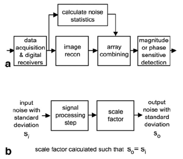
(a) Image reconstruction steps. (b) Individual signal processing step with unity gain for noise SD.

The step-by-step procedure shown in Fig. 2 is described in greater detail in the text below. A summary of signal processing steps is shown in Fig. 3.

FIG. 2.

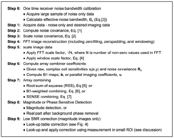
Step-by-Step procedure.

FIG. 3.

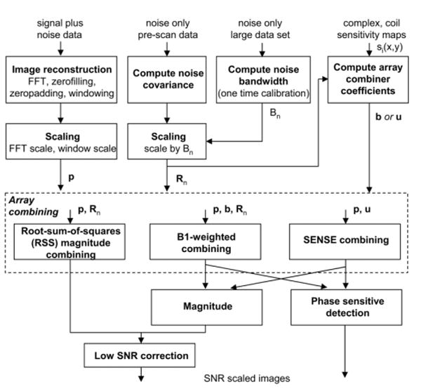
Procedure for SNR scaled image reconstruction (p is complex vector of multi-coil images, b is complex vector of coil sensitivities, u is complex vector of SENSE unmixing coefficients, R_n is noise correlation matrix, and B_n is noise equivalent bandwidth).

Noise Measurement

The noise covariance is measured in order to perform noise scaling and optimum array combining. The method proposed in this article estimates noise statistics from noise only data (i.e., acquired without RF pulses), which may be automatically acquired by the sequence immediately prior to signal acquisition (referred to as pre-scan noise). The noise covariance matrix R_n may be estimated from N pre-scan noise only data samples, n_i(k), k = 1,2,. . . N, acquired simultaneously for all coils (coil index denoted by subscript i). The sample noise covariance matrix R_n is calculated as:

$$R_{ij}=\left(1/N\right){\displaystyle \underset{k=1}{\overset{N}{\Sigma }}}{n}_i^{\ast }\left(k\right)n_j\left(k\right)$$ [1]

where R_ij are components of R_n and n_i(k) is zero mean.

The noise covariance depends on the coil loading and must be measured in vivo for each study or more frequently if the coil positions or loading change. Since the pre-scan noise acquisition and covariance computation are very rapid, the proposed method implements them with every scan; however, the noise may be measured less frequently if the coils are stationary and the loading remains unchanged. Noise scaling based on the measured covariance is applied as part of the array combining step described separately.

The noise covariance measurement is made on the raw noise samples acquired in the full bandwidth; therefore, a noise equivalent bandwidth factor is required in order to scale the image since the input noise spectrum is not flat across the full bandwidth. The noise equivalent bandwidth of a filter is the bandwidth of an equivalent rectangular filter that would produce the same output noise power for white noise input. In other words, if the image is reconstructed using N samples (number of samples integrated by uniform weighted FFT), then the noise variance (σ²) is expected to increase by N. However, since the input noise was non-uniform and the noise samples are not statistically independent, the variance increases by N_effective = B_n N, where B_n defines a noise equivalent bandwidth. The noise covariance must, therefore, be scaled by the noise bandwidth, i.e.

$${\text{R}}_{\text{n scaled}}={\text{R}}_{\text{n}}{/\text{B}}_{\text{n}}.\hspace{0.17em}\hspace{0.17em}$$ [2]

Filtering in the data acquisition electronics and digital receiver occurs in several stages, but the overall response of the combined analog and digital filters determines the noise equivalent bandwidth that must be measured and used in noise scaling. In most systems, the filter response is dictated by the digital receiver, which is typically the most selective filter. The noise equivalent bandwidth of the receiver relative to the sample rate remains fixed as the receiver bandwidth is varied. The noise equivalent bandwidth (6) is easily measured from noise only data by measuring the mean squared value of the average power spectrum, absolute value |H(k)|², normalized by the response at the center,

$$B_n=\left(1/N\right){\displaystyle \underset{k=1}{\overset{N}{\Sigma }}}{|H\left(k\right)|}^2/{|H\left(0\right)|}^2.$$ [3]

Fig. 4 shows the spectrum for noise only input. In this case, 12,288 readouts were acquired with 2× readout oversampling, followed by FFT and averaging. The noise equivalent receiver bandwidth factor is 0.79 for this example, calculated from the spectrum of Fig. 4 as the ratio of mean squared value across the full spectrum to the average value in the central flat portion of the spectrum. Thus, the measured noise covariance R_n must be scaled by 0.79 (i.e., R_{n scaled} = R_n/0.79). The noise bandwidth is fixed by the filter design and only needs to be calibrated a single time. For this reason, a larger number of noise samples is used for greater accuracy and precision.

FIG. 4.

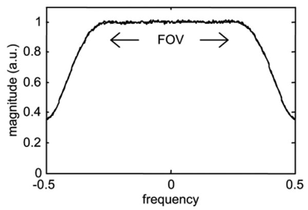
Average noise spectrum.

In systems for which the pre-scan noise is measured using a different bandwidth selection than the subsequent image scan, the noise correlation must be further scaled by the ratio of measurement bandwidths.

FFT Based Image Reconstruction

FFT based image reconstruction may include windowing for reduced Gibb's ringing, zero-filling of missing data, and zero-padding for interpolation. A standard FFT $({\Sigma }_{n=0}^{N-1}x(n)e^{-j2\pi kn/N})$with input white noise having SD = σ will have SD = σ√N after FFT; thus, a scale factor of 1/√N must be applied for unity noise gain (note the value of N is the number of actual data samples and does not include zero-padding or zero-filling). A window function, w(n), must likewise be scaled by its root-mean-squared value, $\sqrt{(1/N)\Sigma w^2(n)}$, such that the input and output have the same noise SD, σ, i.e.:

$$w_{scaled}(n)=w(n)/\sqrt{(1/N)\Sigma w^2(n)}.$$ [4]

Using this formulation, the case of partial k-space acquisition with zero-filling is also handled appropriately. In the case where the input noise spectrum is not flat, the scaling is corrected by using the effective noise bandwidth factor described in the preceding paragraphs.

The resultant scaled, complex, multi-coil image data are written in vector notation as p, comprised of pixel data p_i(x,y) for coil i.

Array Combining

Roemer et al. (7) formulated equations for phased array combined image reconstruction for both root-sum-of squares (RSS) magnitude and optimum B1-weighted combining, and Pruessmann et al. (5) formulated equations for parallel imaging using the image domain SENSE method.

$${\text{SNR}}_{\text{RSS}}=\sqrt{{\text{p}}^T{{\displaystyle {\text{R}}_n}}^{-1}{\text{p}}^{\ast }}$$ [5]

$${\text{SNR}}_{\text{B}1\text{-weighted}}=|{\text{p}}^T{{\displaystyle {\text{R}}_n}}^{-1}{\text{b}}^{\ast }|/\sqrt{{\text{b}}^T{{\displaystyle {\text{R}}_n}}^{-1}{\text{b}}^{\ast }}$$ [6]

$${\text{SNR}}_{\text{SENSE}}=|{\text{u}}^T\text{p}|/\sqrt{{\text{u}}^T{\text{u}}^{\ast }}$$ [7]

Eqs. [5] and [6] for SNR scaled images follow Roemer's formulation, where SNR is the pixel intensity in SNR units, p is the vector of complex image values for each coil, b is the vector of complex coil sensitivities, and R_n is the noise correlation matrix. Note that in Roemer's formulation, the complex pixel values in p have been conjugated. The SNR estimates for the resultant magnitude images are very good at high SNR and may be further corrected to provide a good estimate at low SNR (1,2).

In the case of SENSE (5), described by Eq. [7], u represents the vector of unmixing coefficients that are a reformatting of the unmixing matrix $\text{U}={\left({\text{S}}^{\text{H}}{{\displaystyle {\text{R}}_{\text{n}}}}^{-1}\text{S}\right)}^{-1}{\text{S}}^{\text{H}}{{\displaystyle {\text{R}}_{\text{n}}}}^{-1}$, which contains the optimum noise weighting (S is the coil sensitivity matrix, superscript ^H denotes the Hermitian or conjugate transpose operation). The unmixing vector is reformatted to be applied as a phased array combiner to the full FOV images reconstructed with zero-filling of undersampled data. In the case where relative sensitivities are used, i.e., normalized by RSS combined magnitude $(s_i(x,y)/\sqrt{\Sigma {|s_i(x,y)|}^2}$, s_i(x,y) is coil sensitivity profile for i-th coil), then diag(S^HS) = 1 and the denominator of Eq. [7] $\sqrt{{\text{u}}^T{\text{u}}^{\ast }}$ is equivalent to the g-factor computed from the sensitivities (5) $(g(x,y+kFOV/R)=gk(x,y)=\sqrt{{{\displaystyle {({\text{S}}^H{\text{R}}^{-1}\text{S})}_{(k,k)}}}^{-1}{({\text{S}}^H{\text{R}}^{-1}\text{S})}_{(k,k)}}$ for k-th sub-image, 0 < y < FOV/R, with field-of-view = FOV and k = 0,1,. . . R-1, with R aliased images from uniform undersampling by R). In the preceding, the complex coil sensitivities s_i(x,y) are assumed to be known. Sensitivity estimates may be made using in vivo images acquired separately (5), or adaptively from the images in an auto-calibrating manner (8 –10).

Eqs. [5]–[7] describe the array combining, which incorporates the noise weighting. Using the noise weighting as described along with scaling the signal to preserve the same effective gain as the noise leads to pixel intensities in SNR units. Equivalently, a noise pre-whitening step may be applied by combining channels to create virtual channels that are uncorrelated and have unit variance (11). In the pre-whitening case, the noise weighting is eliminated from the array combining step.

Magnitude Image Correction

Array combining may be implemented according to Eqs. [5]–[7] followed by either magnitude or phase sensitive detection. In the above Eqs. [5]–[7], magnitude images have been assumed. SNR image scaled reconstruction may also be used with phase sensitive detection, in which case the magnitude is replaced by the real part after phase correction for background phase (12). In the case of magnitude detection, an SNR dependent noise correction (1,2) must be applied even though the true input noise SD is used in scaling due to the inherent noise bias in magnitude detection. The noise bias increases with the number of coil elements that are magnitude combined. For example, at SNR = 0 (noise only), the bias is 1.25σ, 1.88σ, 2.74σ, 3.94σ, 5.61σ, and 7.97σ for N_c = 1, 2, 4, 8, 16, and 32 channels, respectively. SNR dependent correction may be implemented by a look-up-table (1,2). Correction curves for low SNR magnitude correction are shown in Fig. 5 for N_c = 1, 2, 4, 8, 16, and 32 combined channels. The correction factor is simply subtracted from the measured SNR. It is worth mentioning that in the case of magnitude detection with B₁-weighted combining or SENSE, the value of N_c = 1, since the multiple channels are combined prior to magnitude detection. For SNR > 10, the correction is less than 5% for up to 4 coils; however, the error without correction increases with a greater number of coils (e.g., >50% error for SNR < 10 using 32 channels). In the case of phase sensitive detection, no correction is required.

FIG. 5.

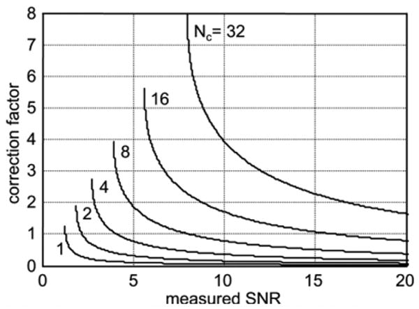
Low SNR magnitude correction curves (N_c = number of channels combined).

A Monte-Carlo simulation of the magnitude bias correction was performed in order to demonstrate the reduction in root mean squared error (RMSE) and to highlight the importance of averaging (small ROI) prior to correction. The simulation was performed using 65,536 noise samples, and was done for both single coil and N_c = 8 coil cases. The mean, SD, and RMSE were calculated for the magnitude with and without correction on both a single-pixel basis and with a 3 × 3 pixel average.

Experimental Validation

Validation of SNR scaled image reconstruction was performed using a time series of 256 phantom images acquired using a Siemens Sonata 1.5T scanner using a single-shot TurboFLASH sequence. Both full k-space imaging with RSS combined magnitude and parallel imaging using acceleration rate 2 SENSE were performed. Pre-Scan noise and raw data were acquired and reconstruction was performed off-line using Matlab. SENSE g-factors (5) were estimated from the pre-scan noise and the B₁-maps and compared with the direct measurement of SD images.

A single-shot turbo-FLASH sequence with very low flip angle was used to minimize signal fluctuations during the approach to steady state. The imaging parameters were: readout flip angle = 2°, TE/TR = 2.7/5.0 ms, bandwidth = 250 Hz/pixel, matrix size 128 × 96, 230 × 172.5 mm² FOV with 8 mm slice thickness. Frequency readout was oversampled corresponding to 2× FOV. Pre-Scan noise was acquired for 30 readouts (30^*256 = 7680 noise samples) acquired in a period of approximately 0.2s using 130 Hz/ pixel bandwidth (7.1 ms per readout). A single axial slice of a cylindrical phantom was imaged for 256 repetitions. A total of 4 coils were used, consisting of 2 elements of the Spine array and 2 elements from the CP Body array (Siemens product coils). For parallel imaging using SENSE, the sequence was custom modified to implement the TSENSE auto-calibration method (10), which uses a cyclic phase encode acquisition order and integrates the undersampled data to obtain a full k-space dataset for estimating B₁-maps.

The sample mean and SD were computed for each pixel using the 256 image frames, and a direct estimate of the SNR was calculated as the ratio of sample mean to sample SD. This direct SNR measurement was then compared to the mean of the SNR scale image reconstructed images, which should be equivalent. Comparison was made by comparing the mean SNR estimates within ROIs at several positions in the phantom. In the case of SENSE accelerated parallel imaging, estimates of g-factor maps were made directly from background noise SD as well as from estimated sensitivity profiles.

In vivo images were acquired using the 32-channel Siemens 1.5T Avanto and a prototype 32-element cardiac array (Invivo Corp). Cardiac imaging of a normal volunteer was performed with informed consent using a breath-held, segmented, ECG triggered, true-FISP cine sequence. Full k-space images were acquired and reconstructed using RSS magnitude combining, as well as accelerated images acquired at rates 2, 3, and 4 and reconstructed using SENSE. B₁-maps were calculated using the auto-calibrating TSENSE method (10). A single, doubly oblique, short-axis slice was acquired with phase encoding performed along the “AP” and “LR” directions for comparison (separate acquisitions). Imaging parameters for phase encoding along the AP direction were: matrix size = 192 × 108, FOV = 320 × 240 mm², slice thickness = 6 mm, readout flip angle = 50°, TE/TR = 1.41/2.82 ms, views per segment = 9, in-plane spatial resolution = 1.7 × 2.2 mm², temporal resolution = 25.4 ms. Breath-Hold durations were 12, 6, 4, and 3 heartbeats for acceleration at rates 1, 2, 3, and 4, respectively. Imaging parameters for phase encoding along the LR direction were: matrix size = 128 × 216, FOV = 240 × 405 mm², slice thickness = 6 mm, readout flip angle = 50°, TE/TR = 1.37/2.74 ms, views per segment = 9, in-plane spatial resolution = 1.9 ×1.9 mm², temporal resolution = 24.7 ms. Breath-Hold durations were 24, 12, 8, and 6 heartbeats for acceleration at rates 1, 2, 3, and 4, respectively. Pre-Scan noise was acquired for 30 readouts. SNR scaled images are shown as an example, although it is not possible to validate using a simple temporal derivative due to cardiac motion; the residual signal after differencing consecutive image frames is shown to illustrate this point. SENSE g-factors were calculated from the raw coil sensitivity maps without spatial smoothing.

Results

SNR scaled image reconstruction and direct measurement of pixel SNR using repeated measurements were compared for phantoms using both RSS magnitude combined imaging and SENSE accelerated parallel imaging. For the case of RSS magnitude combined imaging, Fig. 6 shows (a) mean SNR scaled image (256 trials averaged), (b) SD of SNR scaled images (256 trials), and (c) direct SNR estimate calculated as ratio of mean (a) and SD (b). The SNR images of Figs. 6a and c are in close agreement, window-leveled the same. The mean SNR scaled images of Fig. 6a agree with the SNR measurements of Fig. 6c within 4% in the phantom as measured using a circular ROI of 500 pixels at several locations including the center and edges. The noise SD used in Fig. 6c SNR estimate is based on 256 samples (trials), whereas the noise SD used in Fig. 6a is based on 30 × 256 samples (pre-scan noise) and, therefore, the sample estimate Fig. 6c has greater statistical fluctuation. The noise SD (Fig. 6b) had a mean value = 1.03 within the phantom and 0.73 in a noise only region outside the phantom, representing a 3–4% error. Note that for 4 coils, the noise only region in the magnitude image should have an SD of 0.695. This results in the noise SD image appearing darker in the noise only region outside the phantom. The images have not been pixelwise corrected for magnitude related noise bias. The uncorrected SNR scaled reconstruction (Fig. 6a) has mean = 2.87σ in the noise only region outside the phantom (SNR = 0) where there is a noise bias of 2.74σ (SNR = 0.13 error after correction).

FIG. 6.

Root-Sum-of-Squares (RSS) combined magnitude image reconstruction example: (a) average SNR scaled image (256 trials averaged), (b) SD of SNR scaled images (256 trials), (c) direct SNR estimate computed as ratio of (a) and (b) (note that (a) and (c) are displayed with same window-level and are in close agreement).

For the case of SENSE imaging with acceleration rate = 2, only 4 coils with relatively large size were used to illustrate SNR scaled images with a poor g-factor (g_max ≈ 1.3). Fig. 7 shows the (a) mean SNR scaled image (256 trials averaged), (b) SD of SNR scaled images (256 trials), and (c) direct SNR estimate calculated as ratio of mean (a) and SD (b), with SNR images of Figs. 7a and c window-leveled the same. The SNR scaled reconstruction produces a uniform noise image, as evidenced by uniform SD within the phantom (Fig. 7b). The uniform noise image Fig. 7a after 256 averages clearly shows the spatially dependent loss due to g-factor. The mean SNR scaled images of Fig. 7a agree with the SNR measurements of Fig. 7c within 5% in the phantom as measured using a circular ROI of 128 pixels at several locations including the center and edges in regions with minimum and maximum g-factor.

FIG. 7.

SENSE combined image reconstruction example: (a) average SNR scaled image (256 trials averaged), (b) SD of SNR scaled images (256 trials), (c) direct SNR estimate computed as ratio of (a) and (b) (note that (a) and (c) are displayed with same window-level and are in close agreement).

As previously mentioned, the effective number of channels for magnitude detection after SENSE combining is N = 1, with noise only mean = 1.25σ and noise SD = 0.655σ. The measured noise SD had a mean value 0.68 in a noise only region outside the phantom. The uncorrected SNR scaled reconstruction (Fig. 7a) has mean = 1.31σ in the noise only region outside the phantom (SNR = 0) where there is a noise bias of 1.25σ (SNR = 0.06 error after correction).

Fig. 8a shows a more standard reconstruction weighted by RSS magnitude of sensitivities without scaling for uniform noise. The corresponding noise SD map calculated directly is shown in Fig. 8b. The image of Fig. 8a is scaled by all noise factors with the exception of the SENSE g-factor $(\sqrt{{\text{u}}^T{\text{u}}^{\ast }})$The SENSE g-factor computed directly from the sensitivities shown in Fig. 8c is less noisy than Fig. 8b, both displayed using the same window-level (1 < g < 1.4). In cases such as this with poor g-factor, the uniform noise image of Fig. 7a appears to have an artifact due to the local noise amplification. Therefore, it may be preferable to output the image of Fig. 8a as well as g-map of Fig. 8c. Then the SNR scaled image of Fig. 7a may be derived as the ratio (Fig. 8a image divided by Fig. 8c g-map) for precise SNR measurement, while the output image does not show an intensity variation due to noise enhancement.

FIG. 8.

SENSE combined image reconstruction example: (a) average SNR scaled image without including g-factor term (256 trials averaged), (b) SD of images (256 trials) in (a) is direct estimate of SENSE g-factor, (c) estimate of SENSE g-factor computed from complex coil sensitivities (note that (b) and (c) are displayed with same window-level, 1 < g < 1.4).

Example SNR scaled (uniform noise) cardiac short-axis images are shown in Fig. 9 for acceleration rates 1 through 4 from left to right columns, and with phase encoding along the AP direction (top row) and LR direction (bottom row). Images in Figs. 9a–d (top row) are displayed with the same window and level values. The window and level values for Figs. 9e–h (bottom row) are scaled up by √2 to account for the $\sqrt{2}$SNR increase due to the doubled acquisition time required for LR encoding to achieve approximately the same temporal and spatial resolution. Corresponding g-factor maps based on the coil sensitivity estimates are shown in Fig. 10 for rates 2, 3, and 4, respectively, displayed with the same FOV as Fig. 9. The elliptical ROIs shown in Fig. 10 correspond to the heart region. For phase encoding in the AP direction, 95% of the g-factor values in the heart region of interest are less than 1.03, 1.3, and 2.3, for rates 2, 3, and 4, respectively. For phase encoding in the LR direction, 95% of the g-factor values in the heart region of interest are less than 1.03, 1.1, and 1.25, for rates 2, 3, and 4, respectively. Although the uniform noise SNR scaled images of Fig. 9 have intensity variation due to g-factor variation, this does not appear to be a problem in this range of g-values.

FIG. 9.

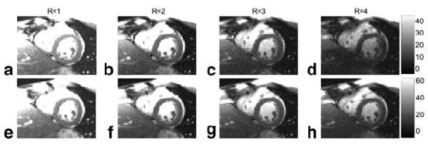
Short-Axis cardiac imaging example of SNR scaled uniform noise reconstructions using full k-space RSS combined magnitude and SENSE acceleration rates 2, 3, and 4 (left to right) with phase encoding direction AP (top row) and LR (bottom row). Note that the bottom row images have approximately $\sqrt{2}$SNR due to the double acquisition time required for LR encoding to achieve approximately the same temporal and spatial resolution.

FIG.10.

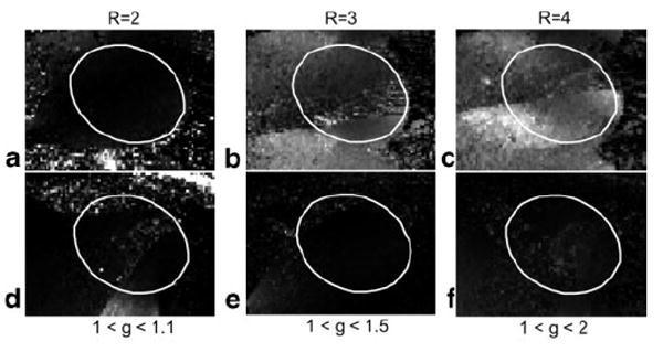
SENSE g-factor computed from raw complex coil sensitivities for rates 2, 3, and 4 (left to right) with phase encoding direction AP (top row) and LR (bottom row) for same cases and FOV as in Fig. 9, with the ellipse corresponding to the heart region.

SNR measurements may be made by simply reading the pixel intensity or using an average value in a region of interest that may be small. For example, at rate R = 1 (i.e., without SENSE acceleration), the SNR in the myocardium of the left ventricle was measured as 30.9 for mid-septal and 22.0 for anterolateral with AP phase encoding (Fig. 9a), and 39.3 and 26.9 for corresponding locations with LR phase encoding (Fig. 9e). This is within 10% of expected after considering the √2 factor for acquisition time and factor of 1.05 for ratio of voxel volumes. The ROI positions were adjusted as closely as possible to be at the same location (12 pixel ROI area) to compensate differences between breath-holds. The measured SNR for AP phase encoding was 30.9, 19.8, 14.2, and 10.5 for mid-septal ROI for rates R = 1, 2, 3, and 4, respectively, indicating a g-factor loss (SNR loss above √R) of 1.1, 1.3, and 1.5 at this location for rates 2, 3, and 4, respectively. The measured SNR for LR phase encoding was 39.3, 26.6, 23.0, and 19.7 for mid-septal ROI for rates R = 1, 2, 3, and 4, respectively, indicating only a few percent difference from expected √R SNR loss at this location for all rates (g-factor ≈1). Correction for noise bias at low SNR may be readily performed by a look-up-table in low SNR regions.

In cardiac imaging, the temporal derivative method of SNR measurement (differencing consecutive frames) is problematic due to motion of the heart. This is illustrated in Fig. 11, which shows two different frames of the magnitude of temporal derivative (a) end-systole and (b) end-diastole to demonstrate that there is significant residual signal, which contaminates a background noise estimate by this method (intensity scale is 0 to 16σ).

FIG. 11.

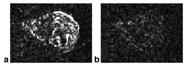
Magnitude of difference between consecutive image frames illustrates contamination of background noise estimate due to motion using this method: (a) end-systolic phase with large residual due to motion, (b) end-diastolic phase with small residual (0 < Δl < 16σ).

Results of a Monte-Carlo simulation of the magnitude bias correction are shown in Fig. 12 for N_c = 1 coil (top row) and N_c = 8 coils (bottom row). The mean value (Figs. 12a and d) has significant bias at low SNR for the uncorrected magnitude (bold), as previously shown (1,2), whereas the bias is reduced after correction. Correction of the average magnitude (dashed) with average of 3 × 3 pixels further reduces the bias as compared with single-pixel correction (normal solid line). However, while the bias correction improves the accuracy, noise in the SNR measurement will affect the precision. The bias correction does in fact result in an increased SD (Figs. 12b and e) as compared to no correction. The RMSE (Figs. 12c and f) provides a combined measure that accounts for both accuracy and precision. For the case of a single coil (N_c = 1), the RMSE for single-pixel correction is comparable to the case without correction, depending on the SNR (slightly better after correction for SNR < 1 and slightly worse after correction, 1 < SNR < 4). With just 3 × 3 pixels averaged, the corrected magnitude has significant improvement as compared with the uncorrected case at low SNR (SNR < 1). For the case of multiple coils (N_c = 8), where the noise bias is more significant, the performance of magnitude bias correction is significantly improved (see Discussion). The RMSE of the corrected magnitude is improved as compared with uncorrected over the full range of SNR, with significant reduction in error at low SNR (SNR < 2), even for single-pixel correction, and improves dramatically with a small amount of averaging.

FIG. 12.

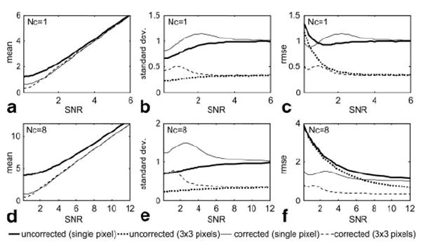
Monte-Carlo simulation results for magnitude noise correction for single-pixel and 3 × 3 pixel average for N_c = 1 and 8 coils. The RMSE provided combined measure of accuracy and precision.

Discussion

The use of pre-scan noise measurement for SNR scaled image reconstruction may be extended to more general image reconstruction algorithms not treated in this article. Any step such as filtering must be scaled to preserve the noise SD. For example, if temporal filtering or interpolation such as sliding window or UNFOLD (13) is used, then the noise equivalent bandwidth of the temporal filter must be accounted for in the scaling (14). In reconstruction that applies spatial filtering or interpolation such as gradient warping correction (15), the local noise statistics are varied and must be compensated for locally by measuring the mean square value of the local interpolation kernel. Extension to iterative reconstruction such as conjugate gradient SENSE (11) as well as extension to k-space domain parallel imaging need to be investigated.

Physiologic noise contributions are not accounted for in the SNR scaled image reconstruction using pre-scan noise, which considers thermal noise sources alone. Physiologic noise is typically measured by time series analysis. By using SNR scaled image reconstructions, it is possible to determine the relative levels of physiologic and thermal noise contributions (16).

Magnitude bias correction may be used to reduce the overall error of the SNR estimate at low SNR. The benefit of bias correction is more significant in the multi-coil case for which there is greater bias. Bias correction is more effective in this case since the low SNR noise distribution is becoming more well behaved, i.e., the chi-squared distribution becomes more normal with an increased number of degrees of freedom. This is also the case using a small degree of spatial averaging (e.g., 3 × 3 pixels), which also alters the noise distribution, becoming more favorable with reduced tails. Importantly, the error in magnitude correction of the proposed method of SNR based image reconstruction using a noise only reference with a large number of noise samples is essentially limited by the inherent noise fluctuation in the magnitude; the magnitude correction error for other schemes may be substantial due to increased fluctuation and biases of background noise estimates.

Finally, care must be taken in noise only acquisition to ensure that there is no RF leakage that will bias the noise measurement. In some vendor systems, the transmitter gain as well as instruction amplitudes must be zeroed.

Conclusion

The proposed image scaling and SNR measurement method is broadly applicable to a number of image reconstruction methods. It has a number of advantages over using a noise only region to estimate background noise. The use of pre-scan noise avoids contamination of the noise region by signal artifact; may use a large number of pre-scan noise samples, which reduces the fluctuation of the noise estimate; and properly accounts for the noise correlation between array elements. The method may be used with parallel imaging such as SENSE for which the noise is locally varying due to the g-factor. SNR measurement using SNR scaled images is both easy and accurate and may be used as ready means for quality control.

References

- 1.Henkelman RM. Measurement of signal intensities in the presence of noise in MR images. Med Phys. 1985;12:232–233. doi: 10.1118/1.595711. [Published erratum in Med Phys 1986;13:544] [DOI] [PubMed] [Google Scholar]
- 2.Constantinides CD, Atalar E, McVeigh ER. Signal-to-noise measurements in magnitude images from NMR phased arrays. Magn Reson Med. 1997;38:852–857. doi: 10.1002/mrm.1910380524. [Published erratum in: Magn Reson Med. 2004 Jul;52:219] [DOI] [PMC free article] [PubMed] [Google Scholar]
- 3.Sijbers J, Den Dekker AJ, Van Audekerke J, Verhoye M, Van Dyck D. Estimation of the noise in magnitude MR images. Magn Reson Imaging. 1998;16:87–90. doi: 10.1016/s0730-725x(97)00199-9. [DOI] [PubMed] [Google Scholar]
- 4.De Wilde JP, Lunt JA, Straughan K. Information in magnetic resonance images: evaluation of signal, noise and contrast. Med Biol Eng Comput. 1997;35:259–265. doi: 10.1007/BF02530047. [DOI] [PubMed] [Google Scholar]
- 5.Pruessmann KP, Weiger M, Scheidegger MB, Boesiger P. SENSE: sensitivity encoding for fast MRI. Magn Reson Med. 1999;42:952–962. [PubMed] [Google Scholar]
- 6.Bendat JS, Piersol AG. Random Data: Analysis and Measurement Procedures. 3. New York: John Wiley & Sons; 2000. [Google Scholar]
- 7.Roemer PB, Edelstein WA, Hayes CE, Souza SP, Mueller OM. The NMR phased array. Magn Reson Med. 1990;16:192–225. doi: 10.1002/mrm.1910160203. [DOI] [PubMed] [Google Scholar]
- 8.McKenzie CA, Yeh EN, Ohliger MA, Price MD, Sodickson DK. Self-calibrating parallel imaging with automatic coil sensitivity extraction. Magn Reson Med. 2002;47:529–538. doi: 10.1002/mrm.10087. [DOI] [PubMed] [Google Scholar]
- 9.Walsh DO, Gmitro AF, Marcellin MW. Adaptive reconstruction of phased array MR imagery. Magn Reson Med. 2000;43:682–690. doi: 10.1002/(sici)1522-2594(200005)43:5<682::aid-mrm10>3.0.co;2-g. [DOI] [PubMed] [Google Scholar]
- 10.Kellman P, Epstein FH, McVeigh ER. Adaptive sensitivity encoding incorporating temporal filtering (TSENSE) Magn Reson Med. 2001;45:846–852. doi: 10.1002/mrm.1113. [DOI] [PubMed] [Google Scholar]
- 11.Pruessmann KP, Wieger M, Boernert P, Boesiger P. Advances in sensitivity encoding with arbitrary k-space trajectories. Magn Reson Med. 2001;46:638–651. doi: 10.1002/mrm.1241. [DOI] [PubMed] [Google Scholar]
- 12.Noll DC, Nishimura DG, Macovski A. Homodyne detection in magnetic-resonance-imaging. IEEE Trans Med Imaging. 1991;10:154–163. doi: 10.1109/42.79473. [DOI] [PubMed] [Google Scholar]
- 13.Madore B, Glover GH, Pelc NJ. Unaliasing by Fourier encoding the overlaps using the temporal dimension (UNFOLD), applied to cardiac imaging and fMRI. Magn Reson Med. 1999;42:813–828. doi: 10.1002/(sici)1522-2594(199911)42:5<813::aid-mrm1>3.0.co;2-s. [DOI] [PubMed] [Google Scholar]
- 14.Kellman P, Sorger JM, Epstein FH, McVeigh ER. Low-latency temporal filter design for real-time MRI using UNFOLD. Magn Reson Med. 2000;44:933–939. doi: 10.1002/1522-2594(200012)44:6<933::aid-mrm15>3.0.co;2-i. [DOI] [PMC free article] [PubMed] [Google Scholar]
- 15.Lai CM. Reconstructing NMR images under non-linear field gradients. J Phys E Sci Instrum. 1983;16:34–38. [Google Scholar]
- 16.de Zwart JA, van Gelderen P, Kellman P, Duyn JH. Application of sensitivity-encoded EPI for BOLD functional brain imaging. Magn Reson Med. 2002 Dec;48:1011–1020. doi: 10.1002/mrm.10303. [DOI] [PubMed] [Google Scholar]