Cardiac Motion Tracking Using CINE Harmonic Phase (HARP) Magnetic Resonance Imaging

Abstract

This article introduces a new image processing technique for rapid analysis of tagged cardiac magnetic resonance image sequences. The method uses isolated spectral peaks in SPAMM-tagged magnetic resonance images, which contain information about cardiac motion. The inverse Fourier transform of a spectral peak is a complex image whose calculated angle is called a harmonic phase (HARP) image. It is shown how two HARP image sequences can be used to automatically and accurately track material points through time. A rapid, semiautomated procedure to calculate circumferential and radial Lagrangian strain from tracked points is described. This new computational approach permits rapid analysis and visualization of myocardial strain within 5-10 min after the scan is complete. Its performance is demonstrated on MR image sequences reflecting both normal and abnormal cardiac motion. Results from the new method are shown to compare very well with a previously validated tracking algorithm.

Major developments over the past decade in tagged cardiac magnetic resonance imaging (1-6) have made it possible to measure the detailed strain patterns of the myocardium in vivo (7-11). MR tagging uses a special pulse sequence to spatially modulate the longitudinal magnetization of the subject to create temporary features, called tags, in the myocardium. Fast spoiled gradient echo imaging techniques are used to create CINE sequences that show the motion of both the anatomy of the heart and the tag features that move with the heart. Analysis of the motion of the tag features in many images taken from different orientations and at different times can be used to track material points in 3D, leading to detailed maps of the strain patterns within the myocardium (11,12).

Tagged MRI has figured prominently in many recent medical research and scientific investigations. It has been used to develop and refine models of normal and abnormal myocardial motion (7,8,12-14) to better understand the correlation of coronary artery disease with myocardial motion abnormalities (15), to analyze cardiac activation patterns using pacemakers (16), to understand the effects of treatment after myocardial infarction (17), and in combination with stress testing for the early detection of myocardial ischemia (18). Despite these successful uses, tagged MRI has been slow in entering into routine clinical use, in part because of long imaging and postprocessing times (19).

Generally, the processing and analysis of tagged MR images can be divided into three stages: finding the left ventricular (LV) myocardium in 2D images, estimating the locations of tag features within the LV wall, and estimating strain fields from these measurements. There has been much creativity in the approaches to these stages. Much work has relied on fully manual contouring of the endocardium and epicardium (20,21), although semiautomated approaches have been proposed as well (22). There is promising recent work on fully automated contouring as well (23). In most cases, contouring results are required for the tag feature estimation stage, for which there are several semiautomated methods available (20,22) and new algorithms that appear very promising for its full automation (23,24).

The third stage in tagged MR image processing, estimation of strain, is largely an interpolation and differentiation computation, and there are several methods described in the literature, including finite element methods (7,20,25), a global polynomial fitting approach (26), and a so-called model-free stochastic estimation approach (10,27). Methods to estimate tag surfaces (25,28,29) represent an intermediate stage between tag identification and strain estimation. Despite the apparent differences between these tagged MRI processing methods, they all share two key limitations: they are not fully automated and they require interpolation in order to form dense strain estimates. This article addresses both of these concerns.

In previous work (30,31), we described a new approach to the analysis of tagged MR images, which we call harmonic phase (HARP) imaging. This approach is based on the use of SPAMM tag patterns (2), which modulates the underlying image, producing an array of spectral peaks in the Fourier domain. It turns out that each of these spectral peaks carry information about a particular component of tissue motion, and this information can be extracted using phase demodulation methods. In (31), we described what might be referred to as single-shot HARP image analysis techniques: reconstructing synthetic tag lines, calculating small displacement fields, and calculating Eulerian strain images. These methods require data from only a single phase (time-frame) within the cardiac cycle, but are limited because they cannot calculate material properties of the motion. In this study, we extend these methods to image sequences—CINE tagged MR images—describing both a material point tracking technique and a method to use these tracked points to calculate Lagrangian strain, including circumferential and radial strain.

The methods proposed in this article are fast and fully automated and use data that can be collected rapidly. It must be clearly understood, however, that at present these methods apply only to 2D images; therefore, the estimated motion quantities must be thought of (and can be rigorously defined as) “apparent” motion, since they represent the projection of 3D motion onto a 2D plane (see Apparent Motion, below). Although the methods can be extended in principle to 3D, dense data acquisition methods must be developed before it would become practical. Despite this present limitation, we believe that the described methods will have immediate clinical impact because the methods are automatic and because circumferential strain is particularly important in the analysis of left ventricular motion.

This article is organized as follows. In the following section, we briefly review both SPAMM tagging and static HARP analysis techniques. In next section, we develop HARP analysis of CINE tagged MR images, describing a method for (apparent) material point tracking and an approach for Lagrangian strain estimation using these tracked points. In Results and Discussion, we demonstrate results using both human and animal data on both normal and abnormal motion. We validate our methods through comparison to existing tag analysis methods. The conclusion is a discussion of these results, their implications, and the possibilities for the future.

MR TAGGING AND HARP IMAGES

SPAMM Tagging

Let I(y, t) represent the intensity of a tagged cardiac MR image at image coordinates y = [y₁ y₂]^T and time t. In this study, we chose y₁ to be the readout direction and y₂ the phase-encoding direction. A typical image showing abnormal motion of a canine heart is shown in Fig. 1a. The left ventricle (LV) looks like an annulus in the center of the image. The effect of tagging can be described as a multiplication of the underlying image by a tag pattern. The pattern appearing in Fig. 1a is a 1D SPAMM tag pattern (stripe) (2), which can be written as a finite cosine series having a certain fundamental frequency (32). Multiplication by this pattern causes an amplitude modulation of the underlying image, which replicates its Fourier transform into the pattern shown in Fig. 1b. The locations of the spectral peaks in Fourier space are integer multiples of the fundamental tag frequency determined by the SPAMM tag pulse sequence. It is also possible to generate a 2D pattern of spectral peaks by using a 2D SPAMM tag pattern. Our approach applies to this case as well.

FIG. 1.

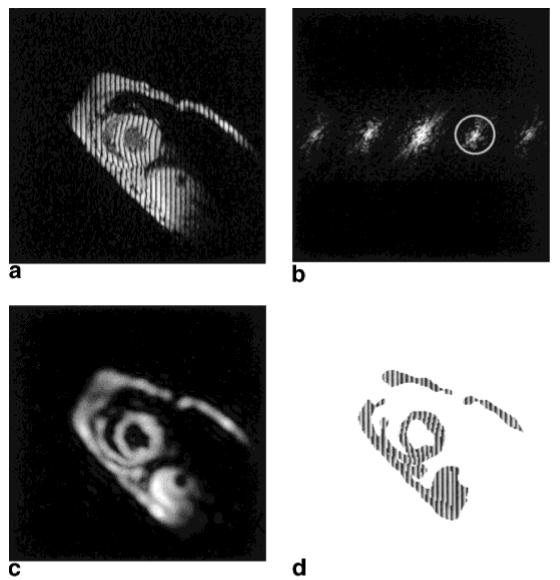
a: An MR image with vertical SPAMM tags. b: Shows the magnitude of its Fourier transform. By extracting the spectral peak inside the circle in b, a complex image is produced with a magnitude (c) and a phase (d).

HARP Imaging

HARP imaging (31) uses a bandpass filter to isolate the k-th spectral peak centered at frequency ω_k—typically the lowest harmonic frequency in a certain tag direction. Thebandpass filter usually has an elliptical support with edges that roll off smoothly to reduce ringing. The contour drawn in Fig. 1b—a circle in this case—represents the -3 dB isocontour of the bandpass filter used to process this data. Once the filter is selected, the same filter is used in all images of the sequence, except that a rotated version is used to process the vertical tagged images. Selection of the filters for optimal performance is discussed in (31). The inverse Fourier transform of the bandpass region yields a complex harmonic image, which is given by:

$$I_k(\mathbf{y},t)=D_k(\mathbf{y},t)e^{j{\varphi }_k(\mathbf{y},t)}$$ [1]

where D_k is called the harmonic magnitude image and ϕ_k is called the harmonic phase image.

The harmonic magnitude image D_k(y, t) reflects both the changes in geometry of the heart and the image intensity changes caused by tag fading. Fig. 1c shows the harmonic magnitude image extracted from Fig. 1a using the filter in Fig. 1b. It basically looks like the underlying image except for the blurring caused by the filtering process. Because of the absence of the tag pattern in the harmonic magnitude image, it can be used to provide a segmentation that distinguishes tissue from background. We use a simple threshold to provide a crude segmentation, where the threshold is selected manually at both end-diastole and end-systole and linearly interpolated between these times.

The harmonic phase image ϕ(y, t) gives a detailed picture of the motion of the myocardium in the direction of ω_k. In principle, the phase of I_k can be computed by taking the inverse tangent of the imaginary part divided by the real part. Taking into account the sign of I_k, the unique range of this computation can be extended to [-π, +π)—using the atan2 operation in C, Fortran, or MATLAB, for example. Still, this produces only the principle value—that is, its “wrapped” value in the range [-π, +π)—not the actual phase, which takes its values on the whole real line in general. We denote this principle value by a_k(y, t); it is mathematically related to the true phase of I_k by:

$$a_k(\mathbf{y},t)=\mathcal{W}\left({\varphi }_k(\mathbf{y},t)\right),$$ [2]

where the nonlinear wrapping function is given by

$$\mathcal{W}\left(\varphi \right)=\mathrm{mod}(\varphi +\pi ,2\pi )-\pi .$$ [3]

Either a_k or ϕ_k might be called a harmonic phase (HARP) image, but we generally use this expression for a_k since, unlike ϕ_k, it can be directly calculated and visualized from the data. Where the two might be confused, however, we refer to ϕ_k as the harmonic phase and a_k as the harmonic phase angle. The HARP angle image corresponding to the spectral peak outlined in Fig. 1b is shown in Fig. 1d. For clarity, it is displayed on a mask created using a crude segmentation of the harmonic magnitude image in Fig. 1c.

Careful inspection of the HARP image in Fig. 1d reveals intensity ramps in the horizontal direction interrupted by sharp transitions caused by the wrapping artifact. The locations of these transitions are very nearly coincident with the tag lines in Fig. 1a, and both reflect myocardial motion occurring during systolic contraction. The intensity ramps in HARP images actually contain denser motion information than what is readily apparent in the original image. For example, calculated isocontours of HARP angle images can produce tag lines throughout the myocardium with arbitrary separation (31). The underlying principle is that both the harmonic phase and the HARP angle are material properties of tagged tissue; therefore, a material point retains its HARP angle throughout its motion. This is the basis for HARP tracking.

Apparent Motion

In tagging pulse sequences, the tag gradients are usually applied in the plane of the image. In this case—which we assume to be true in this article—a tag line appearing in an image at end-diastole is actually part of a tag plane that is orthogonal to the image plane, as shown in Fig. 2a. Since harmonic phase is a material property, the set of points having the same harmonic phase ϕ at end-diastole is also a plane orthogonal to the image plane, and can be considered to be just another type of tab plane. We note that the set of points having the same HARP angle a at end-diastole comprises a collection of parallel planes rather than just a single plane. This creates a problem in HARP tracking, which we address in the following section. To describe apparent motion, however, we need the unique association afforded by the harmonic phase ϕ.

FIG. 2.

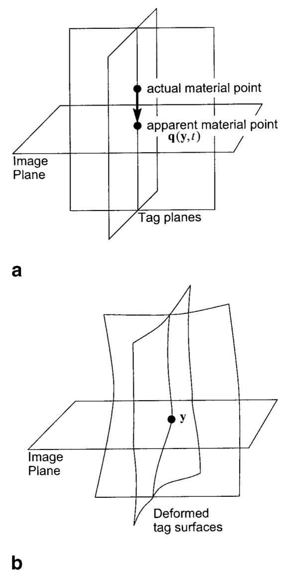
a: Tag planes at end-diastole. b: distortion of the tag planes due to motion.

Given both horizontal and vertical tagged images, it is clear from Fig. 2a that the set of points having the same two harmonic phases at end-diastole comprises a line orthogonal to the image plane intersecting at a single point. As depicted in Fig. 2b, the tag planes distort under motion, causing this line to distort into a curve. Under modest assumptions about the motion, this curve will still intersect the image at a single point. This point can then be uniquely associated with the corresponding point at end-diastole representing an apparent motion within the image plane.

Mathematically, we can describe the apparent motion using an apparent reference map, denoted by q(y, t). This function gives the reference position within the image plane where the point, located at y at time t, apparently was at end-diastole (in the sense that it has the same two harmonic phases). It is clear from Fig. 2—and can be rigorously shown—that q(y, t) is the orthogonal projection of the true 3D material point location at end-diastole onto the image plane. Thus, although calculation of apparent 2D motion has its limitations, it does have a very precise relationship to the true 3D motion. All motion quantities derived from apparent motion, such as strain, can be related to the true 3D quantities in equally rigorous fashion.

HARP PROCESSING OF CINE-TAGGED MR IMAGES

In this section, we describe how to 1) track the apparent motion of points in an image plane, and 2) calculate Lagrangian strain from such tracked points. To arrive at compact equations, we use vector notation. In particular, we define the vectors ϕ = [ϕ₁ ϕ₂]^T, and a = [a₁ a₂]^T to describe pairs of harmonic phase images and HARP angle images, respectively, of the harmonic images I₁ and I₂.

HARP Tracking

Because harmonic phase cannot be directly calculated, we are forced to use its principle value, the HARP angle, in our computations. An immediate consequence is that there are many points in the image plane having the same pair of HARP angles. For a given material point with two HARP angles, only one of the points sharing the same HARP angles in a later image is the correct match—that is, it also shares the same pair of harmonic phases. If the apparent motion is small from one image to the next, then it is likely that the nearest of these points is the correct point. Thus, our strategy is to track apparent motion through a CINE sequence of tagged MR images. We now formally develop this approach.

Consider a material point located at y_m at time t_m. If y_m+1 is the apparent position of this point at time t_m+1, then we must have:

$$\varphi ({\mathbf{y}}_{m+1},t_{m+1})=\varphi ({\mathbf{y}}_m,t_m).$$ [4]

This relationship provides the basis for tracking y_m from time t_m to time t_m+1. We see that our goal is to find y that satisfies:

$$\varphi (\mathbf{y},t_{m+1})-\varphi ({\mathbf{y}}_m,t_m)=0$$ [5]

and then set y_m+1 = y. Finding a solution to Eq. [5] is a multidimensional, nonlinear, root finding problem, which can be solved iteratively using the Newton-Raphson technique. After simplification, the Newton-Raphson iteration is:

$${\mathbf{y}}^{(n+1)}={\mathbf{y}}^{\left(n\right)}-{[\nabla \varphi ({\mathbf{y}}^{\left(n\right)},t_{m+1})]}^{-1}[\varphi ({\mathbf{y}}^{\left(n\right)},t_{m+1})-\varphi ({\mathbf{y}}_m,t_m)]$$ [6]

where ∇ is the gradient with respect to y.

There are several practical problems with the direct use of Eq. [6]. The first problem is that ϕ is not available, and a must be used in its place. Fortunately, it is relatively straightforward to replace the expressions involving ϕ with those involving a. It is clear from Eq. [2] that the gradient of a_k is the same as that of ϕ_k except at a wrapping artifact, where the gradient magnitude is theoretically infinite—practically very large (see also Fig. 1d). As previously shown (31), adding π to a_k and rewrapping shifts, the wrapping artifact by 1/2 the spatial period, leaving the gradient of this result equal to that of ϕ_k whereever the original wrapping artifact occurred. Thus, the gradient of ϕ_k is equal to the smaller (in magnitude) of the gradients of a_k and $\mathcal{W}\left(a_k\right)+\pi$. Formally, this can be written as:

$$\nabla \varphi =\nabla \ast \mathbf{a}$$ [7]

where

$$\nabla \ast \mathbf{a}\equiv \left[\begin{array}{c}\hfill \nabla \ast a_1\hfill \\ \hfill \nabla \ast a_2\hfill \end{array}\right]$$ [8]

and

$$\nabla \ast a_k\equiv \{\begin{array}{cc}\nabla a_k\hfill & \parallel \nabla a_k\parallel \le \parallel \nabla \mathcal{W}(a_k+\pi )\parallel \hfill \\ \nabla \mathcal{W}(a_k+\pi )\hfill & \text{otherwise}\hfill \end{array}\phantom{\}}k=1,2.$$ [9]

A second problem with the use of Eq. [6] is calculation of the difference ϕ(y⁽ⁿ⁾, t_m+1) - ϕ(y_m, t_m), which appears to be impossible since we do not know the phase itself, but only its wrapped version, the harmonic phase. However, provided that |ϕ_k(y⁽ⁿ⁾, t_m+1) - ϕ_k(y_m, t_m)| < π for k = 1, 2—a small motion assumption—it is straightforward to show that:

$$\varphi ({\mathbf{y}}^{\left(n\right)},t_{m+1})-\varphi ({\mathbf{y}}_m,t_m)=\mathcal{W}(\mathbf{a}({\mathbf{y}}^{\left(n\right)},t_{m+1})-\mathbf{a}({\mathbf{y}}_m,t_m)).$$ [10]

Substituting Eq. [7] and Eq. [10] into Eq. [6] provides the formal iterative equation:

$${\mathbf{y}}^{(n+1)}={\mathbf{y}}^{\left(n\right)}-{[\nabla \ast \mathbf{a}({\mathbf{y}}^{n)},t_{m+t})]}^{-1}\mathcal{W}(\mathbf{a}({\mathbf{y}}^{\left(n\right)},t_{m+1})-\mathbf{a}({\mathbf{y}}_m,t_m)).$$ [11]

There are several issues to consider in the implementation of an algorithm based on Eq. [11]. First, because of the phase wrapping the solution is no longer unique; in fact, we can expect a solution y satisfying a(y, t_m+1) = a(y_m, t_m) approximately every tag period in both directions. Thus, it is necessary both to start with a “good” initial point and to restrain the step size to prevent jumping to the wrong solution. Accordingly, we initialize the algorithm at y⁽⁰⁾ = y_m and limit our step to a distance of one pixel. A second issue has to do with the evaluation of a(y, t_m+1) for arbitrary y. Straight bilinear interpolation would work ordinarily; but in this case, the wrapping artifacts in a cause erroneous results. To prevent these errors, we perform a local phase unwrapping of a in the neighborhood of y, bilinearly interpolate the unwrapped angle, and then wrap the result to create an interpolated HARP angle. A final consideration is the stopping criterion. We use two criteria: 1) that the calculated angles are close enough to the desired HARP vector, or 2) that an iteration count is exceeded.

Putting all these considerations together, we can readily define an algorithm that will track a point in one time frame to its apparent position in the next time frame. It is useful to cast this algorithm in a more general framework in order to make it easier to define the HARP tracking algorithm, which tracks a point through an entire sequence of images. Accordingly, we consider y_init to be an initialization from which the search is started, and a* to be a target HARP vector, and t to be the time at which the estimated position ŷ is sought. To track point y_m at time t_m to its apparent position in time t_m+1, we set y_init = y_m, a* = a (y_m, t_m), t = t_m+1, pick a maximum iteration count N, and then run the following algorithm. The result is ŷ, so our desired result is ŷ_m+1 = ŷ.

Algorithm 1 (HARP Targeting)

Let n = 0 and set y⁽⁰⁾ = y_init.

1. If n > N or $\parallel \mathcal{W}(\mathbf{a}({\mathrm{y}}^{\left(n\right)},t)-{\mathbf{a}}^{\ast })\parallel <∊$ then the algorithm terminates with ŷ = y⁽ⁿ⁾.

2. Compute a step direction

   $${\mathbf{v}}^{\left(n\right)}=-{[\nabla \ast \mathbf{a}({\mathbf{y}}^{\left(n\right)},t)]}^{-1}\mathcal{W}(\mathbf{a}({\mathbf{y}}^{\left(n\right)},t)-\mathbf{a}\ast )$$

   using appropriate interpolation procedures.
3. Compute a step size

   $${\alpha }^{\left(n\right)}=\min \left\{\frac{1}{\parallel {\mathbf{v}}^{\left(n\right)}\parallel },1\right\}.$$
4. Update the estimate

   $${\mathbf{y}}^{(n+1)}={\mathbf{y}}^{\left(n\right)}+{\alpha }^{\left(n\right)}{\mathbf{v}}^{\left(n\right)}.$$

5. Increment n and go to step 1.

To track that point through a sequence of images and obtain also ŷ_m+2, ŷ_m+3,..., we successively apply HARP targeting to each image in the sequence. At time t_m+2, the initialization used is ŷ_m+1, the estimated apparent position from the previous time frame; at subsequent time frames this recursive updating of the initialization continues. The target vector, on the other hand, remains the same throughout the entire sequence—given by a* = a(y_m, t_m). This strategy finds a succession of points having the same HARP angles, but (usually) avoids jumping to the wrong solution by keeping the initial point used in HARP targeting near to the desired solution. To formally state this algorithm, suppose that we want to track y_m at time t_m through all images at times t_m+1, t_m+2,..., HARP tracking is given by the following algorithm.

Algorithm 2 (HARP Tracking)

Set a* = a(y_m, t_m), ŷ_m = y_m, and i = m. Choose a maximum iteration threshold N (for HARP targeting).

1. Set y_init = ŷ_i.

2. Apply Algorithm 1 (HARP targeting) with t = t_i+1 to yield ŷ.

3. Set ŷ_i+1 = ŷ.

4. Increment i and go to step 1.

We note that HARP tracking can be used to track points backward in time in exactly the same way as forward. Therefore, it is possible to specify a point in any image at any time and track it both forward and backward in time, giving a complete trajectory of an arbitrary point in space and time.

Lagrangian Strain

Taking the reference time t = 0 to be at end-diastole, HARP tracking allows us to track a material point q at t = 0 to its (apparent) location y at time t (at least for the collection of available image times). This gives us an estimate of the motion map y(q, t). Using y(q, t), it is possible to estimate the deformation gradient tensor F = ▽_qy(q, t) at any material point q and time t using finite differences. The operator ▽_q is the gradient with respect to q. By computing the deformation gradient, most other motion quantities of interest are readily calculated (33). But a more powerful application of HARP tracking is revealed in a somewhat simpler calculation within a semiautomated analysis, which we now describe.

Consider the motion of two material points q_i and q_j. The unit elongation or simple strain is given by:

$$e=\frac{\parallel \mathbf{y}({\mathbf{q}}_i,t_m)-\mathbf{y}({\mathbf{q}}_j,t_m)\parallel }{\parallel {\mathbf{q}}_i-{\mathbf{q}}_j\parallel }-1.$$ [12]

This quantity is zero if the distance between the points remains unchanged, negative if there is shortening, and positive if there is lengthening. To measure circumferential strain at any location within the LV wall we simply place two points along a circle centered at the LV long axis. To measure radial strain we simply place two points along a ray emanating from the long axis. In either case, the strain is measured by tracking the two points using HARP tracking and calculating e. It must be emphasized again that the locations of these points need not be at “tag intersections” or even pixel locations since HARP tracking is fundamentally capable of tracking arbitrary points in the image. This measure of strain has two advantages over the dense calculation of the Lagrangian (or Eulerian strain) tensor. First, it is extremely fast, since only two points need to be tracked instead of the entire image (or region-of-interest). Second, the points are generally placed farther apart than a single pixel, so the elongation calculation is intrinsically less sensitive to noise.

To exploit these advantages, we implemented an approach that tracks points on concentric circles within the myocardium and calculates regional radial and circumferential Lagrangian strain. A simple user interface allows the placement of three concentric circles within the LV wall, as shown in Fig. 3. These circles are manually placed by first clicking on the center of the ventricle—the location of the long axis—and then dragging one circle close to the epicardium and another close to the endocardium. The third circle is automatically placed halfway between these two. Usually the circles are defined on the end-diastolic image, but sometimes it is easier to define them using the end-systolic image because the cross-section of the LV may be more circular. Sixteen equally spaced points are automatically defined around the circumference of each circle, and all 48 points are tracked (forward or backward in time) using Algorithm 2.

FIG. 3.

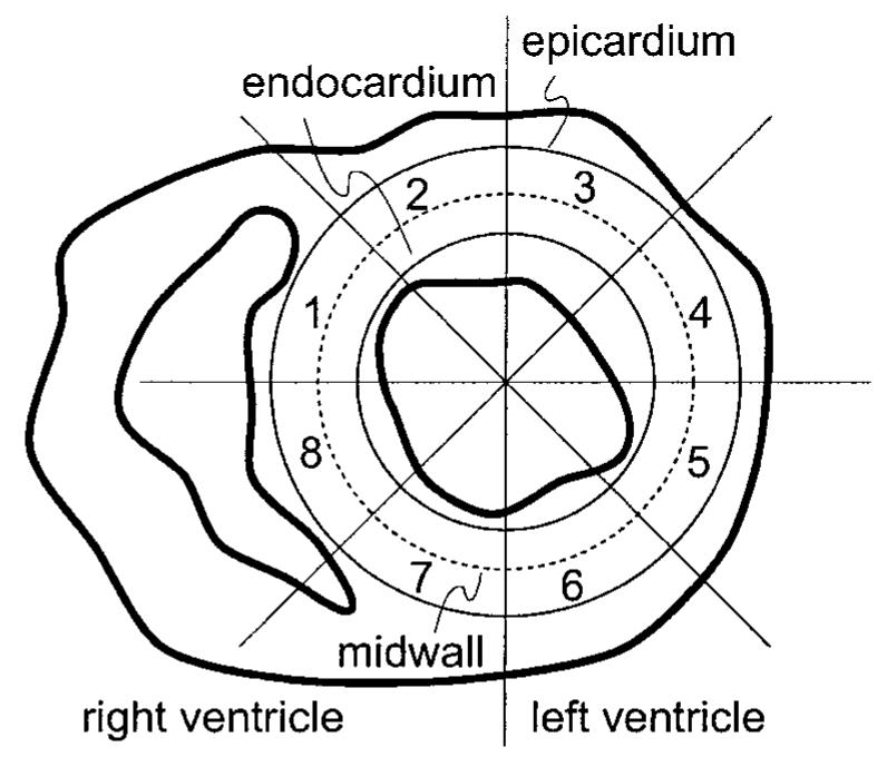
Concentric circles within the LV wall and eight octants.

Strain is computed by measuring the change in distance between neighboring points through the time frames. Regardless of whether the circles were defined at end-diastole or at end-systole (or at any time in between for that matter) the end-diastolic image frame is used as the material reference. The change in distance between points on the same circle corresponds to circumferential strain; change in distance between radially oriented points corresponds to radial strain. Because there are three concentric circles, we can calculat eendocardial, epicardial, and midwall circumferential strain and endocardial and epicardial radial strain. To obtain some noise reduction and for simplicity in presentation, the circles were divided into eight octants and the computed strains were averaged in each of these octants. By convention, the octants were numbered in the clockwise direction starting from the center of the septum, as shown in Fig. 3. The resulting strains are plotted as a function of both time and octant, yielding a spatio-temporal display of cardiac performance within a cross-section.

HARP Refinement

The above procedure requires tracking a collection of points, which ordinarily can be successfully accomplished by applying Algorithm 2 to each point independently. In some cases, however, large myocardial motion or image artifacts may cause a point to converge to the wrong target (tag jumping) at some time frame, causing erroneous tracking in successive frames as well. In this section, we describe a simple approach, which we call refinement, that uses one or more correctly tracked points to correct the tracking of erroneously tracked points.

As stated, Algorithm 2 is initialized at the previous estimated position of the point being tracked. If the in-plane motion between two time frames is very large, however, this initial point may be too far away from the correct solution and it will converge to the wrong point. Refinement is based on the systematic identification of better initializations for Algorithm 2. Suppose it can be verified that one point on a given circle has been correctly tracked throughout all frames. In our experiments, we always found such a point on the septum, where motion is relatively small. We use this point as an “anchor” from which the initializations of all other points on the circle (and possibly all points on all three circles) can be improved and the overall collective tracking result refined.

Starting with the correctly tracked anchor, we define a collection of points separated by less than one pixel on a line segment connecting the anchor with one of its neighbors on the circle. Suppose the anchor is tracked to point y at some particular time. Since by assumption this point is correctly tracked, it is reasonable to assume that the correct tracking result of a point near to the anchor will be near y. Accordingly, we use y as the initial point in Algorithm 2 to track the first point in the collection. We then use this result as the initial point for the second point in the collection, and so on. Upon arriving at the anchor’s first neighbor on the circle, there will have been no opportunity to converge to the wrong result and jump a tag. The neighbor now serves as a new anchor, and the procedure is repeated for the next neighbor on the circle, until all the points on the circle have been tracked.

It is possible to use refinement to “bridge” circles along a radial path and successively correct all three circles. Generally, we have found that tag jumping errors occur only in the free wall, and since refinement is computationally demanding, we generally restrict its operation to a single circle at a time. As a check, we can complete the circle by tracking all the way around and back to the original anchor. If the result is different, then there is a gross error, and it is probably necessary to redefine the circle. Tag fading or other image artifacts can occasionally cause this type of gross error, but it is more likely to be caused by out-of-plane motion. Out-of-plane motion causes the actual tissue being imaged to change. In this case, it is possible that there is no tissue in the image plane carrying the harmonic phase angles corresponding to the point being tracked. In short, the tags may disappear, and the HARP tracking algorithm will simply converge to another point having the correct HARP angles. Because of the particular relationship between the motion and geometry of the LV, we have not found this to be a very significant problem. Since the problem is most likely to occur near the boundaries of the LV, the main limitation it imposes is that we generally must not place our circles very near to the epicardium or endocardium.

EXPERIMENTAL RESULTS AND DISCUSSION

We present the results of three sets of experiments in this section. The first section shows qualitative results using an abnormally paced canine dataset. The second section shows results on a normal human heart under dobutamine stress. The third section describes quantitative comparisons between HARP tracking and a previously validated tracking algorithm called FindTags.

HARP Tracking of a Paced Canine Dataset

To demonstrate the capabilities of HARP tracking, a set of tagged images of an ectopically paced canine heart were used. The strain generated from LV ectopic pacing shows very rapid changes in both time and space. Hence, the strain fields generated are some of the most challenging for the existing strain modeling methods. These data were previously used in a study of cardiac motion under ectopically paced activation using tagged MR imaging and previously proposed analysis techniques. A complete description of the experimental protocol and their results are given in (16). Although our results yield only apparent motion and strain on a single cross-section, rather than giving a complete 3D description, the results we obtain here are very nearly the same as those in (16) and are generated in only a fraction of the time.

Data Description

A pacing lead was sewn onto the epicardial surface of left ventricular basal free wall of a canine heart. MR imaging was performed on a standard 1.5 T scanner with software release 4.7 (General Electric Medical Systems, Milwaukee, WI). A 6 ms SPAMM pulse sequence was used to produce a tag pattern in the myocardium comprising parallel plane saturation bands separated by 5.5 mm in the image plane. The tagging pulse sequence was triggered with a signal from the pacer, and the imaging sequence started 3 ms after the tagging pulses were completed. The image scanning parameters were: TR = 6.5 ms, TE = 2.1, readout-bandwidth = ±32 kHz, 320 mm field of view, 256 × 96 acquisition matrix, fractional echo, two readouts per movie frame and 6-mm slice thickness.

Two sequences of 20 tagged MR short-axis images, one with horizontal tags and the other with vertical tags, were acquired at 14 ms intervals during systole. The images were acquired during breath-hold periods with segmented k-space acquisition, and in this article we use those acquired in a basal plane, near the location of the pacing lead. Figure 4 shows the resulting images cropped to a region of interest around the LV and multiplied together to show vertical and horizontal tags in a single image. Strong early contraction can be seen near the pacing lead on the inferior lateral wall at about 5 o’clock. The septal wall is seen to bow outward in frames 4-8, an abnormal motion called prestretching caused by a delay in the electrical activation signal to the septal region. After this, the entire LV myocardium experiences continued contraction throughout systole in nearly normal fashion.

FIG. 4.

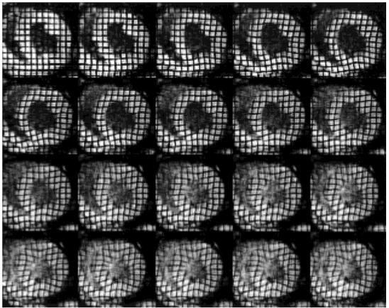
A sequence of tagged MR images of a paced canine heart composed by multiplying the vertical and horizontal tag images to show a grid. The images are 20 time frames depicting the motion of a paced canine heart from end-diastole (top left) to end-systole (bottom right).

HARP Tracking

HARP images were computed from the horizontal tagged image sequence using the bandpass filter depicted in Fig. 1b; a 90° rotated version of this filter was used to compute the vertical HARP images. To demonstrate HARP tracking (Algorithm 2), we selected two tag lines, one vertical and one horizontal, and manually selected a collection of tag points on each. The locations of these points and their individually tracked positions at three later times are shown in Fig. 5. With just one exception, all the points are tracked where one would expect to see them even after considerable tag fading. In particular, both the inward “bowing” of normal contraction and the outward “bowing” of the abnormal prestretching motion are captured very well by HARP tracking. The only incorrectly tracked point can be seen at the top of the image in Fig. 5d. Careful examination of the images shows that out-of-plane motion has caused the horizontal tag line present at the top of the LV in the first time frame to disappear over time. This problem cannot be solved by refinement, unfortunately, but can be avoided by choosing points that are not very near to the myocardial boundaries.

FIG. 5.

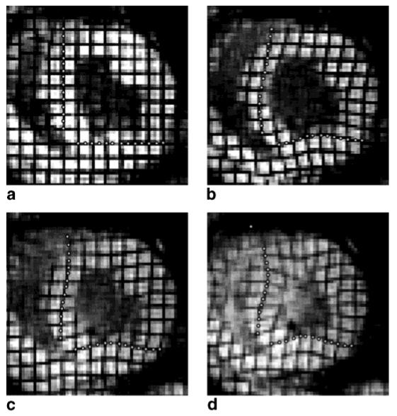
(a) Manually selected points at time frame 1 are tracked through time and displayed at time frames (b) 5, (c) 10, and (d) 20.

To show that HARP tracking is not limited to points on tag lines and to show its potential for calculating strain tensors, a 6 × 6 grid of points separated by one pixel (1.25 mm) was placed in a region bounded by four tag lines in the anterior lateral side of the LV, as shown in Fig. 6a. These points were independently tracked through the full image sequence; Fig. 6b-e shows enlarged pictures of their positions at time frames 1, 5, 10, and 20. Subpixel resolution of tracked points are clearly manifested in the later images, and the underlying local pattern of strain is clearly visible. The pronounced progression of the grid’s shape from a square to a diamond demonstrates very clearly both the radial thickening and circumferential shortening present in normal cardiac motion. It is evident from the regularity of the tracked points that finite differences could be easily used to compute a strain tensor from this data. From this, various quantities related to motion can be computed, including regional area changes and directions of principle strains.

FIG. 6.

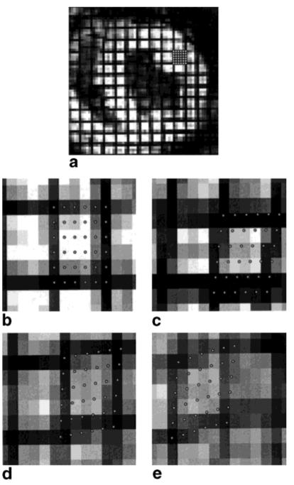
(a) The heart at end-diastole showing the position of the densely picked points; an enlargement of the tracked material points at time frames 1 (b), 5 (c), 10 (d), and 20 (e).

Lagrangian Strain

Next, we computed the regional Lagrangian strain using the procedure described above. Using a user interface, epicardial and endocardial circles were defined. Since the LV looks most circular at end-systole, we used the last image in Fig. 4 to define these circles. The resulting three circles and the defined octants are shown in Fig. 7a. Sixteen points on each circle were tracked backwards in time to end-diastole, resulting in the shapes shown in Fig. 7b. The entire sequence of deformed states is shown in Fig. 7c. From this sequence, we can see that the shape of the LV cross-section starts somewhat elongated, but rapidly becomes circular and then undergoes a mostly radial contraction. We note that it is easy to see that there are no incorrectly tracked points in Fig. 7 because such tag jumps would yield a very distorted contour in one or more time frames.

FIG. 7.

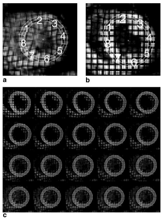
a: Manually defined circles at end-systole. b: The deformed shape of these circles after tracking backwards to end-diastole. c: The entire sequence of tracked circles.

Lagrangian strain profiles were computed for the tracked points depicted in Fig. 7c, as described above. The temporal evolution of radial strain in each octant is shown in Fig. 8a. Positive values indicate myocardial thickening while the negative values indicate thinning. Early myocardial thickening is apparent only in octants 3-6, while octants 8, 1, and 2, show thinning. This is a direct expression of both the early strong contraction taking place in the myocardium nearest the pacing lead and the prestretching of the myocardium on the opposite wall. During time frames 5-10 the myocardium nearest the pacing lead in octants 5-7 relax before contracting a second time toward the strongest radial thickening at end-systole. We note that there is very little apparent difference between epicardial and endocardial radial strain except in quadrant 7, where the endocardial thickening is larger.

FIG. 8.

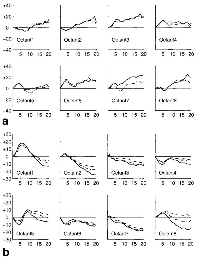
a: The time evolution of epicardial (dot-dashed) and endocardial (solid) radial strain in each octant. b: The time evolution of epicardial (dashed), midwall (dot-dashed), and endocardial (solid) circumferential strain in each octant.

Figure 8b shows the temporal evolution of circumferential strain within each octant. Positive values indicate stretching in the circumferential direction while the negative values indicate contraction. These plots show the same general behavior as in the radial strain profiles. Early contraction in octants 4-6 is seen as a shortening, while octants 8, 1, and 2 show a significant stretching during this same period. After some interval, all myocardial tissues exhibit contractile shortening. These plots also demonstrate a consistently larger endocardial shortening than the midwall, which had more shortening than the epicardium. This agrees with the known behavior of left ventricular myocardium during contraction (13).

Normal Human Heart

In this section, we demonstrate the use of HARP tracking of the cardiac motion of a normal human male volunteer age 27 undergoing a dobutamine-induced (5 μg/kg/min) cardiac stress. We chose this study for demonstration because the very rapid motion of this heart under dobutamine stress requires the use of HARP refinement to correct incorrectly tracked points (see above).

The images were acquired on the same magnet using the same basic imaging protocol as in the canine studies described above. SPAMM tags were generated at end-diastole to achieve saturation planes orthogonal to the image plane separated by 7 mm. Two sets of images with vertical and horizontal tags were acquired in separate breath-holds. Four slices were acquired, but only the midwall-basal slice is used here. Scanner settings were as follows: field of view 36-cm, tag separation 7-mm, 8-mm slice thickness, TR = 6.5 ms, TE = 2.3 ms, 15° tip angle, 256 × 160 image matrix, five phase-encoded views per movie frame.

Figure 9a shows the resulting horizontal and vertical tagged images multiplied together and cropped to a region of interest around the LV. The contours appearing in these images were generated by manually placing epicardial and endocardial circles in the first image and tracking them forward in time using HARP tracking. Because of large motion between the first and second time frames, several points on the anterior wall were mistracked in the second frame. This error was not corrected in the remaining frames because the basic HARP tracking approach uses the previously tracked point as an initialization in the current frame. The result of applying HARP refinement using three manually identified anchors (one on each circle) within the septum is shown in Fig. 9b. By visual inspection, one can see that the refined result has placed the tracked points where one would expect them in each time frame; tag jumping has been eliminated.

FIG. 9.

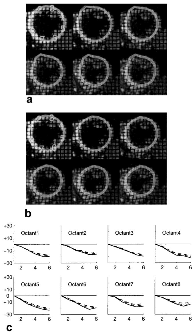
Results from a normal human heart undergoing dobutamine induced stress. a: Short-axis images and tracked circles from first (top-left) to last (bottom-right) without HARP refinement. b: The result after application of HARP refinement. c: The temporal evolution of circumferential strain calculated using the refined points.

Using the refined tracking result, we calculated the temporal evolution of circumferential strain in each quadrant. The result is shown in Fig. 9c. These plots show fairly uniform shortening throughout the LV, with the strongest persistent shortening in the free wall. These results also demonstrate the greatest shortening occurring in the endocardium, as is usual in normal muscle.

Quantitative Comparisons

We have conducted two preliminary analyses of the accuracy of HARP tracking in comparison to an accepted technique known as FindTags (22). The accuracy of FindTags has been shown both in theory and phantom validation to be in the range of 0.1-0.2 pixels, depending on the contrast-to-noise ratio (CNR) of the image (34,35). Our results strongly suggest that the accuracy of HARP is approximately the same as FindTags. It is emphasized that the following experiments report comparative results on tracking tag lines and tag crossings because FindTags is limited to the tracking of these features; HARP has no such limitations and can be used to track arbitrary points within the myocardium or elsewhere.

Finding Tag Lines

Using data from a normal human subject, we used FindTags to estimate both the contours (endocardium and epicardium) and the tag lines in 27 images from a vertical tagged, short axis dataset comprising nine-image sequences from three short-axis slices within the LV. We generated HARP images from these nine images using the first harmonic and a bandpass filter similar to the one shown in Fig. 1b. Theory predicts that tag brightness minima should be located at a phase angle of π radians, and therefore π isocontours of HARP images should be very close to the tag points identified by FindTags. Figure 10a superposes tag points from FindTags onto these HARP isocontours in a mid-ventricular image taken at the seventh time frame, where significant tag fading has occurred.

FIG. 10.

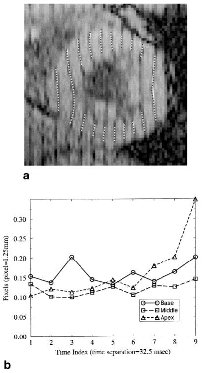
HARP accuracy in comparison to FindTags using normal human data. a: A tagged image with tag points from FindTags (black dots) overlaying HARP π isocontours (white curves). b: Average distance between the FindTags tag points and the HARP isocontour.

There appear to be only minor differences between HARP isocontours and tag contours estimated using FindTags. HARP appears to yield a very slightly smoother result, the main difference being a slight fluctuation around the HARP result on the free wall (3 o’clock). It is hard to say which is more visually satisfying. We note that the average HARP angle calculated using the entire collection of FindTags tag points is indeed π to three significant digits, verifying the theoretical prediction that tag valleys should have a HARP angle of π. We note that local phase unwrapping was required in order to compute this average angle since π corresponds exactly to the location of a wrapping artifact in HARP images.

To arrive at a quantitative measure of accuracy, we calculated the distance between each tag point and the nearest HARP π radian isocontour in the same image. Plots of the root-mean-square (rms) distances as a function of time for the basal, mid-ventricle, and apical short-axis images are shown in Fig. 10b. Since FindTags does not represent the truth and since we do not know the exact FindTags rms error for this dataset, however, it is only possible to give a rough bound on the actual HARP rms error. For example, in the first time frame, the rms distance between FindTags and HARP is approximately 0.13 pixel. The rms error of FindTags alone is estimated to be 0.10 pixel, based on the CNR of the images and previous validation studies (34). A straightforward calculation then shows that the HARP rms error is in the range 0.03-0.23 pixel. The extremes are possible, however, only if the errors from HARP and FindTags are perfectly correlated (either negatively or positively), which is very unlikely. Also unlikely, but arguably closer to correct, would be that the respective errors are uncorrelated. In this case, the expected rms error of HARP would be approximately 0.08 pixel. Similar numerical results hold for the remaining time frames, suggesting that HARP tracking errors are approximately the same as those of FindTags.

Finding Tag Crossings

HARP tracking uses two HARP images simultaneously, and is rather more like finding tag line crossings than tag lines themselves. So in this experiment, we compare HARP tracking with tag line crossing estimation using FindTags. Using the paced canine heart data described above, we used FindTags to compute the positions of all tag lines, both vertical and horizontal, in the 20-image basal short-axis image sequence. Using the endocardial and epicardial contours, also estimated using FindTags, we computed the tag line intersections falling within the myocardium. We then ran HARP tracking on each of these points seeking the target vector a = [π π]^T radians, including the first time-frame.

The rms distance between the FindTags intersections and the HARP tracked points is shown as a function of time in Figure 11. We observe that these errors are somewhat larger than the previous experiment. This can be mostly accounted for by noting that when seeking two lines instead of just one, the error should go up by approximately √2. Other minor differences can be accounted for by the different experimental setups and imaging protocols. The general trend of increasing distance over time is also to be expected because the signal-to-noise ratio drops as the tags fade.

FIG. 11.

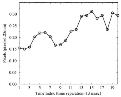
Root mean square difference in tag crossing estimation between Findtags and HARP.

One interesting feature in the plot in Fig. 11 is the “hump” occurring in time frames 4-7. It is reasonable to conclude that the presence of this hump is caused by the dramatic motion taking place over this time period—strong contraction in the inferior lateral wall and prestretching in the septum—but the specific mechanism for this performance difference between the two approaches is unclear. It is possible that FindTags errors are increasing, as it is known that changes in the tag profile due to contraction and stretching degrade the performance of the underlying matched filter. It is also possible that HARP errors are increasing, perhaps because the spectral changes associated with the motion are not completely captured by the HARP bandpass filter. Further analytic and experimental evaluation is needed to identify and quantify these subtle differences in performance; this is a subject for future research.

Computation Speed

All the computations, including the HARP tracking method and the Lagrangian strain computations, were done on a 400 MHz Intel Pentium II processor using MATLAB (Math-works, Natick, MA). Despite the fact that we have not optimized our MATLAB code (to eliminate loops, for example) HARP processing is very fast in comparison to other methods that we are aware of. For the paced canine heart, computation of 20 vertical and 20 horizontal HARP images took about 30 sec. Positioning endocardial and epicardial circles within the LV myocardium takes about 20 sec of human interaction. Tracking the 48 points defined by this process through all 20 time-frames took only about 5 sec, and the computation of the Lagrangian strain also took about 5 sec. The overall time from images to strain takes only about 2 min, which includes time to click on buttons and arrange images. There is potential for significant streamlining of certain steps, as well. It is worth mentioning that for the same dataset it would take more than 1 hr to track the tag lines using FindTags.

The organization of image data and the definition of the bandpass filters also adds time to the overall processing time of HARP analysis. On standard scans these times are negligible, and the image sequences can be constructed automatically and preset bandpass filters can be used. On special scans or new experimental protocols, some additional time must be spent in preparing the data for HARP processing. An experienced user can generally perform these additional steps in less than 30 min, and a convenient user interface will reduce this time even further. After further validation and optimization, HARP will certainly be feasible for clinical use.

Notes on Optical Flow

We previously suggested a method for computing optical flow, a dense incremental velocity field, using HARP images (31). This HARP optical flow method used the idea of the HARP angle as a material property and the notion of apparent motion, but it did not iteratively seek the point sharing two HARP values. In fact, Eq. [11] can be thought of as the successive application of the basic optical flow calculation of (31) in order to obtain an increasingly better solution. If HARP tracking were applied to every pixel in an image and tracked only to the next time frame, it would give the same basic result as optical flow only with greater accuracy. HARP tracking would also require a factor of 4-5 times longer, since that is the number of iterations typically used before satisfying the termination criterion. There may be applications for use of the fast and dense optical flow calculation, however. Rapid visualization of flow fields, intelligent feedback of tag pattern frequency based on the motion pattern, or interactive modification of bandpass filters are possibilities.

CONCLUSION

In this article, the material property of HARP angle was exploited to develop a 2D HARP tracking method that is fast, accurate, and robust. Points were tracked in a coordinate system that was used to directly compute both circumferential and radial Lagrangian strain in the left ventricle. Experiments on a paced canine heart demonstrated the ability for HARP to track abnormal motion and to compute strains that are consistent with previously reported analyses. A refinement technique for the correction of incorrectly tracked points was developed and demonstrated on a normal human heart undergoing dobutamine stress. Finally, a preliminary error analysis was conducted showing that HARP tracking compares very favorably with FindTags, a standard template matching method. HARP tracking and Lagrangian strain analysis was shown to be computationally very fast, amenable to clinical use after suitable further validation.

REFERENCES

- 1.Zerhouni EA, Parish DM, Rogers WJ, Yang A, Shapiro EP. Human heart: tagging with MR imaging—a method for noninvasive assessment of myocardial motion. Radiology. 1988;169(1):59–63. doi: 10.1148/radiology.169.1.3420283. [DOI] [PubMed] [Google Scholar]
- 2.Axel L, Dougherty L. MR imaging of motion with spatial modulation of magnetization. Radiology. 1989;171:841–845. doi: 10.1148/radiology.171.3.2717762. [DOI] [PubMed] [Google Scholar]
- 3.McVeigh ER, Atalar E. Cardiac tagging with breath-hold cine MRI. Magn Reson Med. 1992;28:318–327. doi: 10.1002/mrm.1910280214. [DOI] [PMC free article] [PubMed] [Google Scholar]
- 4.Fischer SE, McKinnon GC, Maier SE, Boesiger P. Improved myocardial tagging contrast. Magn Reson Med. 1993;30:191–200. doi: 10.1002/mrm.1910300207. [DOI] [PubMed] [Google Scholar]
- 5.Atalar E, McVeigh ER. Minimization of dead-periods in MRI pulse sequences for imaging oblique planes. Magn Reson Med. 1994;32(6):773–777. doi: 10.1002/mrm.1910320613. [DOI] [PMC free article] [PubMed] [Google Scholar]
- 6.Fischer SE, McKinnon GC, Scheidegger MB, Prins W, Meier D, Boesiger P. True myocardial motion tracking. Magn Reson Med. 1994;31:401–413. doi: 10.1002/mrm.1910310409. [DOI] [PubMed] [Google Scholar]
- 7.Young AA, Axel L. Three-dimensional motion and deformation of the heart wall: estimation with spatial modulation of magnetization—a model-based approach. Radiology. 1992;185:241–247. doi: 10.1148/radiology.185.1.1523316. [DOI] [PubMed] [Google Scholar]
- 8.Moore C, O’Dell W, McVeigh E, Zerhouni E. Calculation of three-dimensional left ventricular strains from biplanar tagged MR images. J Magn Reson Imaging. 1992;2(2):165–175. doi: 10.1002/jmri.1880020209. [DOI] [PMC free article] [PubMed] [Google Scholar]
- 9.Park J, Metaxas D, Axel L. Analysis of left ventricular wall motion based on volumetric deformable models and MRI-SPAMM. Med Image Anal. 1996;1(1):53–71. doi: 10.1016/s1361-8415(01)80005-0. [DOI] [PubMed] [Google Scholar]
- 10.Denney TS, Jr, McVeigh ER. Model-free reconstruction of three-dimensional myocardial strain from planar tagged MR images. J Magn Reson Imag. 1997;7:799–810. doi: 10.1002/jmri.1880070506. [DOI] [PMC free article] [PubMed] [Google Scholar]
- 11.McVeigh ER. Regional myocardial function. Cardiol Clin. 1998;16(2):189–206. doi: 10.1016/s0733-8651(05)70008-4. [DOI] [PubMed] [Google Scholar]
- 12.McVeigh ER. MRI of myocardial function: motion tracking techniques. Mag Reson Imag. 1996;14(2):137. doi: 10.1016/0730-725x(95)02009-i. [DOI] [PubMed] [Google Scholar]
- 13.Clark NR, Reichek N, Bergey P, Hoffman EA, Brownson D, Palmon L, Axel L. Circumferential myocardial shortening in the normal human left ventricle. Circulation. 1991;84:67–74. doi: 10.1161/01.cir.84.1.67. [DOI] [PubMed] [Google Scholar]
- 14.McVeigh ER, Zerhouni EA. Noninvasive measurements of transmural gradients in myocardial strain with MR imaging. Radiology. 1991;180(3):677–683. doi: 10.1148/radiology.180.3.1871278. [DOI] [PMC free article] [PubMed] [Google Scholar]
- 15.Lugo-Olivieri CH, Moore CC, Guttman MA, Lima JAC, McVeigh ER, Zerhouni EA. The effects of ischemia on the temporal evolution of radial myocardial deformation in humans. Radiology. 1994;193:161. [Google Scholar]
- 16.McVeigh ER, Prinzen FW, Wyman BT, Tsitlik JE, Halperin HR, Hunter WC. Imaging asynchronous mechanical activation of the paced heart with tagged MRI. Magn Reson Med. 1998;39:507–513. doi: 10.1002/mrm.1910390402. [DOI] [PMC free article] [PubMed] [Google Scholar]
- 17.Lima JA, Ferrari VA, Reichek N, Kramer CM, Palmon L, Llaneras MR, Tallant B, Young AA, Axel L. Segmental motion and deformation of transmurally infarcted myocardium in acute postinfarct period. Am J Physiol. 1995;268(3):H1304–12. doi: 10.1152/ajpheart.1995.268.3.H1304. [DOI] [PubMed] [Google Scholar]
- 18.Croisille P, Judd RM, Lima JAC, Moore CC, Arai RM, Lugo-Olivieri C, Zerhouni EA. Combined dobutamine stress 3D tagged and contrast enhanced MRI differentiate viable from non-viable myocardium after acute infarction and reperfusion. Circulation. 1995;92(8):I–508. [Google Scholar]
- 19.Budinger TF, Berson A, McVeigh ER, Pettigrew RI, Pohost GM, Watson JT, Wickline SA. Cardiac MR imaging: report of a working group sponsored by the National Heart, Lung, and Blood Institute. Radiology. 1998;208(3):573–576. doi: 10.1148/radiology.208.3.9722831. [DOI] [PubMed] [Google Scholar]
- 20.Young AA, Kraitchman DL, Dougherty L, Axel L. Tracking and finite element analysis of stripe deformation in magnetic resonance tagging. IEEE Trans Med Imaging. 1995;14(3):413–421. doi: 10.1109/42.414605. [DOI] [PubMed] [Google Scholar]
- 21.Amini AA, Chen Y, Curwen RW, Mani V, Sun J. Coupled B-snake grids and constrained thin-plate splines for analysis of 2-D tissue deformations from tagged MRI. IEEE Trans Med Imaging. 1998;17(3):344–356. doi: 10.1109/42.712124. [DOI] [PubMed] [Google Scholar]
- 22.Guttman MA, Prince JL, McVeigh ER. Tag and contour detection in tagged MR images of the left ventricle. IEEE Trans Med Imaging. 1994;13(1):74–88. doi: 10.1109/42.276146. [DOI] [PubMed] [Google Scholar]
- 23.Denney TS. Identification of myocardial tags in tagged MR images without prior knowledge of myocardial contours. In: Duncan J, Gindi G, editors. Proc Inf Proc Med Imaging. 1997. pp. 327–340. [Google Scholar]
- 24.Kerwin WS, Prince JL. Tracking MR tag surfaces using a spatiotemporal filter and interpolator. Int J Imag Sys Tech. 1999;10(2):128–142. [Google Scholar]
- 25.Moulton MJ, Creswell LL, Downing SW, Actis RL, Szabo BA, Vannier MW, Pasque MK. Spline surface interpolation for calculating 3-D ventricular strains from MRI tissue tagging. Am J Physiol (Heart Circ Physiol) 1996;270:H281–H297. doi: 10.1152/ajpheart.1996.270.1.H281. [DOI] [PubMed] [Google Scholar]
- 26.O’Dell WG, Moore CC, Hunter WC, Zerhouni EA, McVeigh ER. Three-dimensional myocardial deformations: calculations with displacement field fitting of tagged MR images. Radiology. 1995;195:829–835. doi: 10.1148/radiology.195.3.7754016. [DOI] [PMC free article] [PubMed] [Google Scholar]
- 27.Denney TS, Prince JL. Reconstruction of 3-D left ventricular motion from planar tagged cardiac MR images: an estimation theoretic approach. IEEE Trans Med Imaging. 1995;14(4):625–635. doi: 10.1109/42.476104. [DOI] [PubMed] [Google Scholar]
- 28.Kerwin WS, Prince JL. Cardiac material markers from tagged MR images. Med Image Anal. 1998;2(4):339–353. doi: 10.1016/s1361-8415(98)80015-7. [DOI] [PubMed] [Google Scholar]
- 29.Amini A, Huang J, Klein A. Flexible shapes for segmentation and tracking of cardiovascular data; Proc IEEE Int Conf Image Proc; IEEE Comp Soc Press. 1998.pp. 5–9. [Google Scholar]
- 30.Osman NF, Prince J. Direct calculation of 2D components of myocardial strain using sinusoidal MR tagging; Proc SPIE Med Imag Conf; 1998.pp. 142–152. [Google Scholar]
- 31.Osman NF, Prince JL. Motion estimation from tagged MR images using angle images; Proc Int Conf Imag Proc; Chicago: Comp Soc Press. 1998.pp. 704–708. [Google Scholar]
- 32.Shinnar M, Leigh JS. Inversion of the Bloch equation. J Chem Phys. 1993;98(8):6121–6128. [Google Scholar]
- 33.Gurtin ME. An introduction to continuum mechanics. Academic Press; New York: 1981. [Google Scholar]
- 34.Atalar E, McVeigh ER. Optimization of tag thickness for measuring position with magnetic resonance imaging. IEEE Trans Med Imaging. 1994;13(1):152–160. doi: 10.1109/42.276154. [DOI] [PMC free article] [PubMed] [Google Scholar]
- 35.Moore CC, Reeder SB, McVeigh ER. Tagged MR imaging in a deforming phantom: photographic validation. Radiology. 1994;190:765–769. doi: 10.1148/radiology.190.3.8115625. [DOI] [PMC free article] [PubMed] [Google Scholar]