Diffraction-Biased Shear Wave Fields Generated with Longitudinal Magnetic Resonance Elastography Drivers

Abstract

Magnetic Resonance Elastography (MRE) is a technique for quantifying the acoustic response of biological tissues to propagating waves applied at low frequencies in order to evaluate mechanical properties. Application-specific MRE drivers are typically required to effectively deliver shear waves within the tissue of interest. Surface MRE drivers with transversely oriented vibrations have often been used to directly generate shear waves. These drivers may have disadvantages in certain applications, such as poor penetration depth and inflexible orientation. Therefore, surface MRE drivers with longitudinally oriented vibrations are used in some situations. The purpose of this work was to investigate and optimize a longitudinal driver system for MR elastography applications. It is shown that a cone-like hemispherical distribution of shear waves are generated by these drivers and the wave propagation is governed by diffraction in the near field. Using MRE visualization of the vector displacement field, the properties of the shear wave field created by longitudinal MRE drivers of various sizes were studied to identify optimum shear wave imaging planes. The results offer insights and improvements in both experimental design and imaging plane selection for 2-D MRE data acquisition.

Introduction

Measurement of motion with MR in medical applications was originally directed at blood flow measurement and vascular imaging (1–4). Dynamic Magnetic Resonance Elastography is a technique in which propagating shear waves are generated in tissue, typically by an external mechanical driver, and the waves are imaged using a modified phase-contrast technique (5,6). The oscillating cyclic motion-encoding gradients (MEG) that are used to allow visualization of the shear waves in tissue are synchronized with the mechanical driver via trigger pulses or some other method. The maximum phase shift measured at each pixel in the resulting phase-contrast MR images is proportional to the scalar product of the displacement amplitude vector, the motion-encoding gradient vector and the number of gradient pairs (5,6). By adjusting the phase offset between the mechanical excitation and the oscillating magnetic gradient, wave images can be obtained at various phases of the wave cycle. Typically, 4–8 phase offsets are sampled for one cycle of motion. This allows for an extraction of the harmonic component of the motion at the driving frequency, giving the amplitude and the phase of the harmonic displacement at each point in space, which is used in most MR elastography inversion algorithms (7,8).

Drivers with transverse motions have often been used to directly generate planar shear waves parallel to the coupling surface (5,9), as indicated schematically in Figure 1 (a). In some applications, transverse drivers provide insufficient penetration depth and a lack of design flexibility for shear motion orientation. Therefore, longitudinal drivers applying cyclic longitudinal vibrations were developed to overcome these limitations (10–17). However, even with a simple geometry, longitudinal drivers do not generate simple planar shear waves parallel to the contact surface, like those seen with conventional transverse drivers (for example, the shear wave projection along the direction parallel to the driving surface indicated in Figure 1 (b)). Consequently, the objectives of our study were: (1) to better understand the mechanism of wave formation for application-specific longitudinal MRE drivers from theory and by wave component analysis; (2) to visualize and quantitatively delineate the diffraction-biased field of shear waves within an isotropic homogeneous medium; and (3) to optimize imaging planes for 2-D MRE using longitudinal drivers by investigating the wave field properties and the reliability of shear stiffness estimates in different imaging planes.

Figure 1. Comparison of transverse and longitudinal MRE drivers.

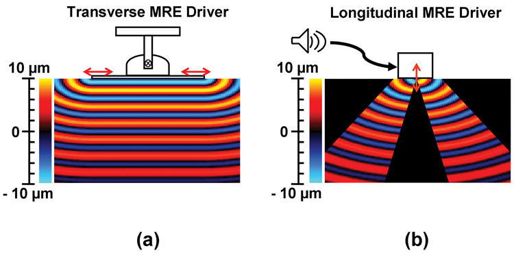
(a): A direct shear driver applies cyclic transverse vibrations (shown as the red double-headed arrows) to the surface of an object. A planar shear wave is generated within the homogeneous medium.

(b): A longitudinal driver generates longitudinal vibrations (shown as the red double-headed arrow) to the surface of an object. A cone-like hemispherical shear wave field is generated in the homogeneous medium.

The color bars indicate the particle shear displacement (in micrometers) along the horizontal direction. (positive motion is assumed from the left to the right)

Theory

Consider a finite circular disk of radius a vibrating normal to the surface of a semi-infinite isotropic homogeneous medium. An analytical solution in the near field can be developed for the problem of shear wave generation. The harmonic force excitation of circular frequency ω from the finite circular disk applies a uniform stress P_ine^iωt on the surface of the medium in the circular region of r < a. The solution has been addressed by Miller and Pursey (18), and is frequently cited by many authors. In the medium, the wave equation is given by Miller and Pursey (19–23), as shown in Equation (1).

$$(\lambda +2\mu )\nabla \nabla \cdot \overrightarrow{u}-\mu \nabla \times \nabla \times \overrightarrow{u}=\rho \frac{{\partial }^2\overrightarrow{u}}{\partial t^2}$$ (1.)

Here, $\overrightarrow{u}$ is the displacement vector, ρ is the density of the medium, ∂/∂t denotes a derivative with respect to time, and λ and μ are the Lame constants of the linear viscoelastic medium. The generated wave field may be regarded as comprising three parts: a compression wave, a shear wave and a surface or Rayleigh wave (5,24).

While soft tissues are generally neither isotropic nor linear, for this work it is impractical for the following derivations to be based on a more exact and comprehensive mechanical description of real tissues. Therefore, the mechanical properties used will be those approximating the gel phantoms used in the accompanying experiments. The further assumption of low attenuation results in the following equation relating the shear wave speed (c) to the material density (ρ) and the “shear stiffness” (μ):

$$\mu =c^2\rho$$ (2.)

To derive expressions for the compression and shear waves, whose wave surfaces are spherical in form, Miller and Pursey used the spherical polar coordinate system with the center of the disk as the origin. For the following equations, the time dependence e^iωt is assumed but omitted for clarity, and the displacement vector is $\overrightarrow{u}={[u_R{u}_{\theta }{u}_{\varphi }]}^T.$ For the case of large R and small a, the radial and transverse components of the displacement u_R and u_θ are

$$\begin{array}{c}\frac{u_R}{P_{in}}\approx -\frac{a^2}{2\mu }\frac{e^{-iR}}{R}\frac{\text{cos}\theta ({\eta }^2-2{\text{sin}}^2\theta )}{F_0(\text{sin}\theta )}\hfill \\ \frac{u_{\theta }}{P_{in}}\approx -\frac{i{a}^2{\eta }^3}{2\mu }\frac{e^{-i\eta R}}{R}\frac{\text{sin}2\theta \sqrt{{\eta }^2{\text{sin}}^2\theta -1}}{F_0(\eta \text{sin}\theta )}\hfill \end{array}$$ (3.)

Where

$$\begin{array}{c}{F}_0(\zeta )={(2{\zeta }^2-{\eta }^2)}^2-4{\zeta }^2\sqrt{{\zeta }^2-{\eta }^2}\sqrt{{\zeta }^2-1}\hfill \\ \eta =\frac{k_2}{k_1},k_1=\omega \sqrt{\frac{\rho }{\lambda +2\mu },}{k}_2=\omega \sqrt{\frac{\rho }{\mu }}\hfill \end{array}$$ (4.)

k₁ and k₂ are the wave numbers for compression and shear wave propagation, respectively.

Considering the surface wave, Miller and Pursey derived an expression in the cylindrical polar coordinate system. Due to the cylindrical symmetric properties, we have $\overrightarrow{u}={[u_r{u}_{\phi }{u}_z]}^T$ with u_φ = 0 and derivatives with respect to φ vanish. The following are wave propagation equations in the r and z directions at any location on the surface or within the medium (z ≥ 0).

$$\begin{array}{c}\\ \begin{array}{c}\frac{u_z}{P_{in}}=\frac{a}{\mu }{\int }_0^{\infty }\frac{J_1(\zeta a{k}_1)\sqrt{{\zeta }^2-1}}{F_0(\zeta )}\{2{\zeta }^2{e}^{-z{k}_1\sqrt{{\zeta }^2-{\eta }^2}}+({\eta }^2-2{\zeta }^2)e^{-z{k}_1\sqrt{{\zeta }^2-1}}\}{J}_0(\zeta r{k}_1)d\zeta \hfill \\ \frac{u_r}{P_{in}}=\frac{a}{\mu }{\displaystyle {\int }_0^{\infty }\frac{J_1(\zeta a{k}_1)\zeta }{F_0(\zeta )}\{2\sqrt{{\zeta }^2-1}\sqrt{{\zeta }^2-{\eta }^2}{e}^{-z{k}_1\sqrt{{\zeta }^2-{\eta }^2}}+({\eta }^2-2{\zeta }^2)e^{-z{k}_1\sqrt{{\zeta }^2-1}}\}{J}_1(\zeta r{k}_1)d\zeta }\hfill \end{array}\end{array}$$ (5.)

where J₀ and J₁ are Bessel functions of the first kind. The variable ζ is used to denote integration over the wave number domain which has been normalized with respect to k₁. The asymptotic solutions of (Equation 5) for large R and small a are

$$\begin{array}{c}\frac{u_z}{P_{in}}\approx \frac{a^2{e}^{-(1/4)i\pi }}{\mu F_0\text{'}(p)}\sqrt{\frac{\pi k_{1}p(p^2-1)}{2r}}{e}^{-i{k}_{1}pr}\{2p^2{e}^{-k_{1}z\sqrt{p^2-{\eta }^2}}+({\eta }^2-2p^2)e^{-k_{1}z\sqrt{p^2-1}}\}\hfill \\ \frac{u_r}{P_{in}}\approx \frac{a^2{e}^{(1/4)i\pi }}{\mu F_0\text{'}(p)}\sqrt{\frac{\pi k_1{p}^3}{2r}}{e}^{-i{k}_{1}pr}\{2\sqrt{p^2-1}\sqrt{p^2-{\eta }^2}{e}^{-k_{1}z\sqrt{p^2-{\eta }^2}}+({\eta }^2-2p^2)e^{-k_{1}z\sqrt{p^2-1}}\}\hfill \end{array}$$ (6.)

Where p is defined as the positive root of the equation F₀(ζ) = 0, which is a function of the Poisson’s ratio of the medium. When p has been determined, the value of F₀'(p)is most easily obtained from the formula.

$$F_0\text{'}(p)=8p\{(2p^2-{\eta }^2)-\frac{{(2p^2-{\eta }^2)}^2}{4p^2}-\frac{2p^4(2p^2-{\eta }^2-1)}{{(2p^2-{\eta }^2)}^2}\}$$ (7.)

These expressions can be used to model the ideal condition of a point source (equivalent to the case of large R and small a) vibrating normally to the free surface of a semi-infinite isotropic medium. For a point source, if the Poisson’s ratio of the incompressible material is assumed to be 0.5, it has been shown experimentally that a maximum diffraction angle of the shear waves of 35° occurs (25).

The wave expressions for the compression, shear and surface waves from an arbitrarily shaped driver can be modeled by summing contributions from numerous point-source elements of the driver. Constant stress is assumed over the region of the surface beneath each radiating element. While a useful guide, in practice the shear wave fields generated by longitudinal MRE drivers have not been systematically evaluated and proper understanding of the wave fields produced is crucial to obtaining accurate shear stiffness values.

Methods

Data were collected to investigate the properties of the wave fields produced by longitudinal MRE drivers and to determine optimal imaging planes for 2-D MRE.

Figure 2 illustrates the experimental setup. A function generator was triggered to produce synchronized sinusoidal waves which were power amplified to 17.6 volts peak-to-peak amplitude and input into a 30-cm diameter active audio speaker that was located at least 3 meters away from the magnet bore. The speaker was enclosed in a stiff plastic box to channel the pressure variations into a 2.5-cm diameter outlet. A drum-shaped passive longitudinal driver was connected to the speaker via a 6-m long plastic tube 2.5-cm in diameter. The driver was made of stiff plastic (6-mm acrylic) except for the top surface which was made of a soft flexible material and could be acoustically driven at low frequencies (20–200 Hz) to give longitudinal vibrations. In this study, two different sized cylindrical longitudinal drivers were used: one was 3-cm in diameter, 7-cm in height and its top surface was made of polycarbonate Lexan with 0.25-mm thickness; the other one was 8-cm in diameter, 5-cm in height and its top surface was made of a polycarbonate sheet with 0.5-mm thickness. The driver sizes were far less than the wavelength of the acoustic pressures used (1.7–17 m). Therefore, it is reasonable to assume that a uniform pressure is exerted on both pneumatic drivers. A cylindrical 15% B-Gel (from bovine skin powder, SIGMA Chemical Company, St. Louis, MO) phantom 25-cm in diameter and 6.2-cm in height was used as an isotropic homogeneous medium simulating soft tissues.

Figure 2. Schematic diagram of the experimental setup for MR Elastography system.

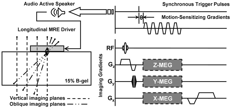
Phantom experiment set-up. Low-frequency longitudinal acoustic waves were generated by an audio speaker and then conducted into the cylindrical passive longitudinal MRE driver as shown in the upper left part of the figure. A cylindrical 15% B-gel phantom was placed against the vibrating surface of the longitudinal driver as shown in the bottom left. The dotted lines and dash-dotted lines indicate the vertical and oblique imaging planes for the MRE image acquisitions, respectively. The GRE MRE pulse sequence is shown at the bottom right. The cyclic motion-sensitizing gradients and the acoustic driver are synchronized using trigger pulses provided by the imager (upper right). The phase offset (θ) between the two can be adjusted. As shown by the shaded regions, the motion-sensitizing gradients can be applied along any desired axis to detect cyclic motion in that direction.

All experiments were performed on a 1.5 T whole-body GE imager (Signa, GE Medical System, Milwaukee, WI) using the body coil.

Both longitudinal MRE drivers were used for each experiment. In a preliminary experiment, the resonance frequency of the experimental setup was determined to be 100 Hz and 90 Hz for the 3-cm and 8-cm drivers respectively.

The resonance frequencies were chosen as operating frequencies for each driver in the following experiments. The shear stiffness of the phantom was assessed at 20 °C and 4 °C (cooler to stiffen the gel) with a conventional transverse driver. Planar shear waves were obtained using a 2-D MRE acquisition and the corresponding mean shear stiffness value in multiple imaging planes orthogonal to the driving surface were regarded as gold standards for the following experiments since MRE results in these types of gel phantoms has already been validated with dynamic mechanical testing (26,27).

1. Wave component analysis and visualization

To investigate the wave components generated from the longitudinal MRE drivers, 2-D MRE data with three orthogonal MEGs were analyzed to obtain quiver plots of the wave fields. The Cylindrically symmetric experimental setup ensured that a central imaging plane (a plane passing through the central axis of the driver and perpendicular to the surface of the driver) sensitized in three orthogonal motion directions in space (X, Y and Z) is adequate to delineate the wave field generated by the longitudinal MRE drivers. By using Matlab (Version 7.0.1, The Mathworks, Inc.), three dimensional cyclic motion was visualized by quiver plot animations, which showed the particle motion for every sampling volume within the central imaging plane. This provided a method to compare experimental data with the wave equations and corresponding solutions reported by Miller and Pursey.

2. Dependence of wave amplitude and shear stiffness on imaging plane

To investigate the dependence of wave amplitude and stiffness measurements on the choice of imaging plane, multiple imaging planes were selected for 2-D MRE acquisitions. The phantom was imaged at room temperature (20 °C) using a 2-D GRE MRE sequence (7). In order to reduce the scanning time, the longitudinal MRE driver was operated continuously with the TR set to an integer multiple of the wave period (40 ms for 100-Hz motion, 33.3 ms for 90-Hz motion). The TE was set to a minimum value of 14.7 ms for the 100-Hz experiments and 15.8 ms for the 90-Hz experiments. The other MRE imaging parameters included a 26-cm FOV, 256×64 acquisition matrix, 30° flip angle, 10-mm slice thickness, and one pair of 1.76-G/cm cyclic trapezoidal MEG synchronized to the longitudinal driver by using a trigger provided by the scanner. The trigger timing was varied to obtain wave images of 8 different phase offsets during one motion cycle.

Vertical imaging planes (located at distances d 0 to 60 mm from the central axis of the driver at 10-mm increments) and oblique imaging planes (tilted at angles θ 0° to 60° from the central axis at 10° intervals) were obtained to study the spatial properties of the wave field. For each imaging plane, the MEGs were applied successively in the three orthogonal directions of space. A coordinate system aligned with each imaging plane was used throughout the experiments and defined as: 1) X-MEG: in-plane from left to right and parallel to the acoustic coupling surface; 2) Y-MEG: in-plane perpendicular to X; 3) Z-MEG: through-plane and perpendicular to the slice. Compared to the Cartesian coordinate system typically used in MRI, spherical polar coordinates are much more suitable for describing the wave field produced by this type of driver, as indicated in Equation (3), because both the compression and shear waves propagate semi-spherically. Furthermore, the desired shear motion is not simply in the horizontal direction (parallel to the vibrating surface) as it is for planar waves Instead, it is perpendicular to the shear wave propagation direction, which might deviate from the vertical central axis depending on the properties of the driver and the object under investigation.

The mean displacement amplitude and the mean shear stiffness (using the Direct Inversion algorithm (25,28–31)) were calculated in all shear wave images by using a standardized region of interest (square ROI, 20×20 pixels) positioned 15-mm below the driving surface.

3. Diffraction quantification of the biased shear wave fields

To investigate the diffraction properties of the generated shear wave fields from each driver, 2-D MRE data were obtained with various driving frequencies and material stiffness. X-MEG phase difference images were obtained with each driver in an imaging plane passing through the central axis of the driver and orthogonal to its vibrating surface. The same MRE parameters as above were used except that the mechanical driving frequency was varied from 20 Hz to 200 Hz in 10 Hz increments. The corresponding TR times were adjusted to maintain continuous wave illumination. The protocol was repeated first with the phantom at room temperature (20 °C), and then again after the phantom was cooled to 4 °C to stiffen it.

Quantitative displacement maps were calculated from the wave images of 8 phase offsets. Diffraction angles of the shear wave fields were estimated by tracing the maximum acoustic energy flow on the displacement maps. Using the measured diffraction angle, shear stiffness estimates were obtained at 20 °C and 4 °C by acquiring oblique images tilted at an angle equal to the measured diffraction angle α with Z-MEG.

Results

The gold standard shear stiffness of the 15% B-gel phantom, measured using a traditional transverse driver, was 2.67 ± 0.06 kPa at 20 °C, and 23.7 ± 0.8 kPa at 4 °C. The displacement components in the direction parallel to the driving surface were calculated using Equation (3) for two different sized circular pistons within a semi-infinite medium (incompressible material with Poisson ratio of 0.5), and shown in the polar plots and 3-D renderings in Figure 3. These two theoretical results demonstrate that this component of the shear motion distribution from a piston driver is expected to be cylindrically symmetric about the central axis where a cone-shaped blind zone of decreased displacement is observed. Furthermore, the width of the cone-shaped blind zone appears to be governed by diffraction. That is, the angle of divergence decreases when the size of the vibrating source increases. The perpendicular component of the motion from Equation (3) has significant contributions from both the shear and longitudinal motion, especially under the driver. The shear component stems from the superposition of shear wave fronts coming from the distributed source of a non-point-source driver. Since it is not practical to separate the shear from the longitudinal information in these equations, renderings equivalent to those in Figure 3 do not yield any useful insights into the properties of the shear wave motion.

Figure 3. Theoretical shear wave diffraction from longitudinal MRE drivers.

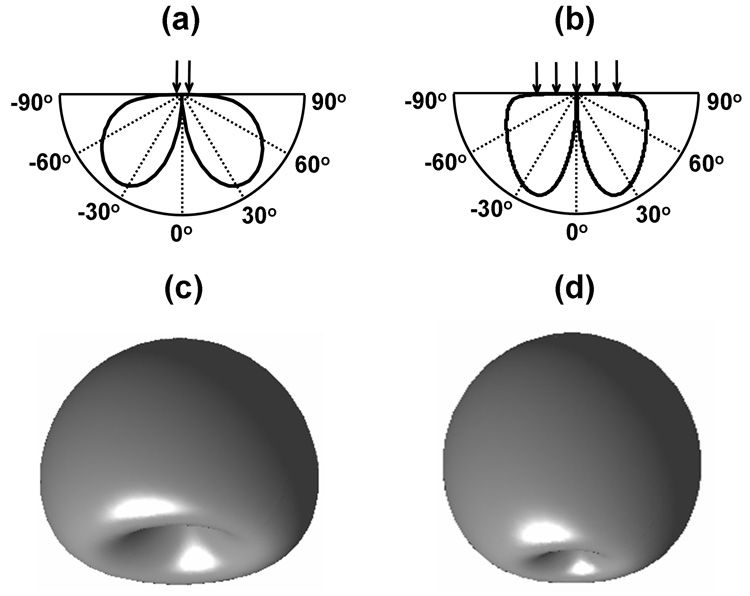
The two polar plots in (a) and (b) illustrate the horizontal component of the shear displacement field directivities of a point source and a circular source, respectively, in the far field from the Miller and Pursey’s theory. Shear displacement projection along the direction parallel to the driving surface were also calculated in a semi-infinite medium and presented in plots of (c) and (d).

1. Wave component analysis and visualization

Figure 4 shows in multiple vertical imaging planes the X and Z polarizations of the vector wave field produced by the 3-cm and 8-cm longitudinal drivers. No substantial through-plane motion (Z direction) was detected within the central imaging plane for either driver. Therefore, it is sufficient for wave component analysis in the central imaging plane to depend on only the two orthogonal in-plane components of motion (X and Y directions) visualized in the quiver plots shown in Figure 5. Four different phase offsets selected from a harmonic motion cycle are demonstrated in Figure 5(b) for the 3-cm and 8-cm drivers.

Figure 4. Measured shear wave fields from longitudinal MRE drivers.

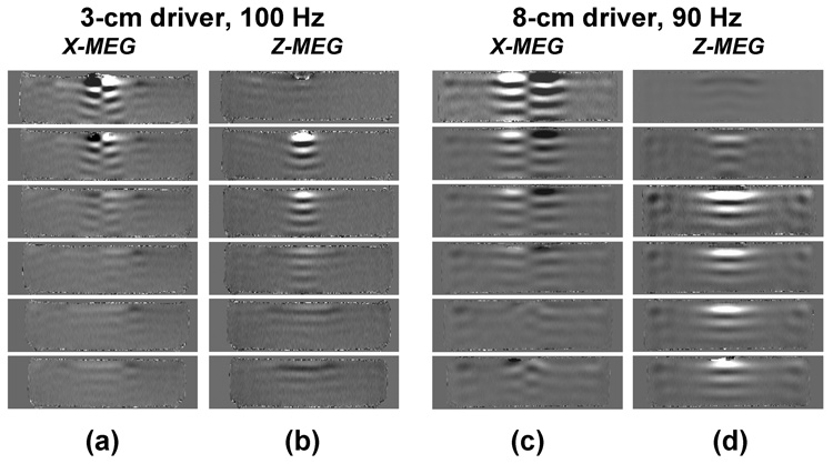
Shear wave images in multiple vertical imaging planes (distanced from 0 to 50 mm) using X-and Z-MEG for 3-cm and 8-cm drivers respectively.

Figure 5. Wave field visualizations.

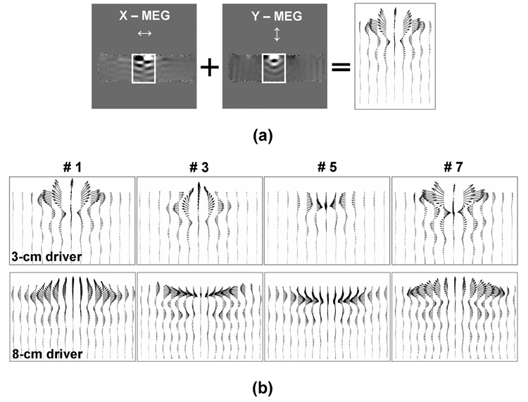
(a): Wave images in the central imaging plane perpendicular to the surface of the driver using X-and Y-MEG. The rectangular ROI shown in the two images was then chosen for the wave visualization as a 2-D quiver plot, which indicates both the motion magnitude and direction for each sampling volume.

(b): For both the 3-cm and 8-cm drivers, quiver plots from four phase offsets equally spaced over one period of motion were chosen for delineating the cyclic in-plane motions of the generated wave field.

The observed spatially and temporally varying motion vectors indicate a very complex waveform, which is composed of transverse and elliptic waves. Each vector in Figure 5 indicates the shear wave motion, and also the elliptic Rayleigh wave motion within one wavelength of the surface. Meanwhile, the motion vectors along the central axis give the appearance of a compression wave propagating with a similar velocity to the shear waves due to the superposition of the wave motion vectors.

When considering the wave images using the X-MEG direction in Figure 4, two out-of-phase lobes of shear waves were observed in all imaging planes as shown in the left column of Figure 4 (a) and (b). They are separated by a certain diffraction angle α with no obvious shear motion observed along the central axis. The shear motion was found to be maximal in the central imaging plane and then decreased as the imaging planes moved to the distal end of the phantom.

Considering the wave images using the Z-MEG direction in Figure 4, no obvious shear motion was observed within the central imaging plane. One lobe of planar shear waves was observed in all the other imaging planes as shown in the right column of Figure 4 (a) and (b), and the maximum shear displacement was found at a vertical imaging plane located approximately 1/4 diameter from the driver center.

2. Shear stiffness measurements in multiple imaging planes

Figure 6 shows the wave amplitude and stiffness estimates from a standardized ROI 15 mm beneath the surface of the driver in several vertical and oblique imaging planes. Although the shear waves were detectable in all the X-MEG images, the shear stiffness estimations did not show consistency. For different vertical imaging planes, as shown in Figure 6 (a) and (b), the shear stiffness estimates for the 3-cm driver decreased to a minimum 20 mm from the central axis and then increased as the imaging plane moved to the distal end. However, with the 8-cm driver, the estimates were fairly stable around 2.68 ± 0.03 kPa 0–30 mm from center, and then increased as the imaging planes moved further away. For different oblique X-MEG imaging planes, as shown in Figure 6 (c) and (d), the shear stiffness measurement was minimum in the 0° oblique planes for both drivers, and then increased dramatically when the imaging plane tilted further away from vertical.

Figure 6. Wave amplitude and stiffness estimates in different imaging planes.

Mean displacement and shear stiffness (using X- and Z-MEG data) were measured in multiple vertical or oblique imaging planes for the two different sized drivers. For each displacement/shear stiffness plot in (a), (b), (c) and (d), the horizontal axis indicates either the image plane location from the central axis of the driver or degree of obliqueness of the plane from vertical. All measurements were taken by using an ROI of 20×20 pixels placed 15 mm away from the surface of the driver.

Inconsistency of the shear stiffness estimates was also observed in the Z-MEG wave images. For different vertical imaging planes, as shown in Figure 6 (a) and (b), the estimated shear stiffness for the 3-cm driver decreased to a minimum 30 mm from the central axis and then increased as the imaging plane moved to the distal end. The shear stiffness measurements for the 8-cm driver were fairly stable around 2.67 ± 0.02 kPa within 0–30 mm of the central axis. For different oblique imaging planes, as shown in Figure 6 (c) and (d), the shear stiffness measurement was minimum in the 10° and 0° oblique planes for the 3-cm and 8-cm drivers, respectively, and increased dramatically when the imaging plane obliqueness increased.

3. Diffraction quantification of the biased shear wave fields

Figure 7 (a) illustrates the method of diffraction quantification by tracking the propagation direction of acoustic energy using MRE displacement maps. The four different wave image examples in Figure 7 (b) show the diffraction phenomena via X-MEG wave images in the central imaging plane with phantoms of two different stiffnesses and two different sized drivers. Diffraction quantification demonstrated that the diffraction angle increased when either the phantom stiffness increased, the driving frequency decreased, or the driver size decreased as shown in Figure 7 (c). In order to combine all these factors, the relative aperture size (the ratio between the driver size and the wavelength of the shear waves) was used. Agreement was observed among all four curves as shown in Figure 7 (d). That is, the diffraction angle increased when the relative aperture size decreased. Furthermore, a diffraction angle of approximately 0° was observed if the relative aperture size was greater than 4.

Figure 7. Diffraction analysis for various driver sizes, frequencies and material stiffnesses.

(a): Illustration of the technique to quantify the diffraction angle α for each experiment. The left half of the image shows an X-sensitized phase difference image in the central imaging plane. The right half shows the displacement map corresponding to the detected cyclic shear motions from 8 phase offsets. The white dotted lines indicate the direction of maximum motion amplitude as determined from the amplitude map and defined the diffraction angle α.

(b): Four different wave images for quantifying the diffraction angles for various driver sizes and material stiffnesses. The diffraction pathways are all marked as red lines and demonstrate that the diffraction increases when either the driver size decreases or the shear stiffness increases.

(c): This plot shows the measured diffraction angle as a function of motion frequency for each set of experiments. This indicates that the diffraction angle decreases when the vibration frequency increases in each case. However, the data from these four cases do not correlate with each other.

(d): This plot shows the relationship between the diffraction angle and the relative aperture size for each set of experiments. All four cases agree well with each other when normalized in this fashion.

Oblique Z-MEG wave images tilted with an angle equal to the diffraction angle α yielded stiffness estimates near the gold standard: for the 3-cm driver at 20°C, the stiffness estimate was 2.68 ± 0.09 kPa in a 12° oblique plane; for the 3-cm driver at 4°C, the stiffness estimate was 23.6 ± 0.6 kPa in a 25° oblique plane; for the 8-cm driver at 4°C, the stiffness estimate was 24.0 ± 0.7 kPa in a 21° oblique plane; and for the 8-cm driver at 20°C, the stiffness estimate was 2.67 ± 0.02 kPa in the vertical plane (0° oblique) distanced 20 mm from the central axis in order to avoid the null region along the central axis and to obtain maximum shear displacement.

Discussion

It has been demonstrated that the optimal acquisition orientation for a single-slice, single-direction, 2-D MRE analysis using a longitudinal driver is an imaging plane oriented along the angle of diffraction of the shear waves with through-plane (Z) motion-sensitizing gradients. The diffraction angle was shown to be dependent on the relative aperture size of the experiment, which depends on the driver size and the shear wavelength in the medium. The results were demonstrated in a series of phantom experiments.

1. Analysis of the shear wave field

The homogeneous phantom used in these experiments approximates a semi-infinite medium in the near field, ignoring wave reflections and interference. In the wave propogation theory presented, longitudinal drivers do not generate only shear waves within a semi-infinite space. They generate longitudinal waves and Rayleigh waves as well.

Transverse waves (i.e. shear waves) are waves with motion perpendicular to their propagating direction. The generated shear waves observed here had bilateral directivities, as has been observed by other researchers (25,28–31), and did not propagate simply along two parallel straight lines. Instead, they were prone to deviate from the center axis and formed a biased diffraction field. It was anticipated that in these experiments the particle motion would be orthogonal to the direction of the wave normal and, because of the spherical and cylindrical symmetries of the experiment, shear waves might be observed using any or all three orthogonal motion-sensitizing directions. As shown in Figure 5 (a), the particle shear motion vector had nonzero components in both the X and Y motion-sensitizing directions, with the X-MEG data best depicting the diffraction angle of the field.

The acoustic longitudinal waves propagate very rapidly in tissue and tissue-like media (~ 1540 m/s in the 15% B-gel phantom) and have very long wavelengths (~ 10 m). Therefore, even with Y-MEG, it is difficult to study them using MRE. In the Y-MEG wave data shown in Figure 5 (a), a wave is observed that has a component of motion along the direction of wave propagation, yet has the wavelength of a shear wave due to the vector summation of the cylindrically symmetric shear motion of the driver. This wave was less apparent with the larger driver (larger relative aperture size), which indicated that the Y-MEG data would not be very robust for 2-D MRE analysis.

Rayleigh waves are surface waves with a similar velocity to shear waves (C_Rayleigh ≈ 0.95×C_shear) (19). MRE is able to visualize Rayleigh waves that are also superimposed on the shear waves. This wave energy, which propagates along the surface of the gel, produces elliptical motion consisting of both horizontal and vertical components that are detected using either X or Y motion-sensitizing gradients. However, Rayleigh waves do not propagate far into a medium and are attenuated within approximately one wavelength of the surface (19). The elliptical Rayleigh waves are depicted via in-plane wave vector visualization as shown in the quiver plots of Figure 5 (a).

In wave images using X-MEG, the phase difference signal was composed of two wave components: the projections of both the shear and Rayleigh wave motion. The images show two out-of-phase wave lobes indicating opposite particle motion directions anti-symmetric about the central axis. No substantial shear motion was detected along a central vertical line or cone area (the blind zone determined by diffraction). It was further demonstrated by the 2-D quiver plots in Figure 5 that only the vertical (Y) component of motion was detected in that central area. This motion propagated forward at the same velocity as the shear waves as described above.

In wave images with Y-MEG, the phase difference accumulation was caused by all 3 wave components: bulk longitudinal motion and projections of both shear and Rayleigh waves. Usually, bulk longitudinal motion can be removed from the wave images with high pass filters. Shear wave illumination of soft tissue using Y-MEG is limited because the wave energy is focused primarily within the diffraction cone. Because the diffraction angle for soft tissues is typically less than about 35° for soft tissues (and near 0° for large relative aperture sizes), shear stiffness estimation and further investigation of shear waves were discouraged in the wave images of Y-MEG.

2. Optimum imaging plane selection for shear stiffness measurement

Besides comparing with the gold standard stiffness values in these experiments, the planar nature of the shear waves was also regarded as an important criterion for optimum imaging plane selection. From the shear wave patterns in the wave images with X-MEG and Z-MEG, we found a cone-shaped blind zone of low shear displacement along the central axis when using X-MEG. The problem becomes more severe with increasing amounts of diffraction, and it inevitably causes artifacts in the resulting elastograms because of the loss of wave information. Also, the out-of-phase, bimodal wave field in the X-MEG images produces a discontinuous wave field that can also produce artifacts in the elastograms. Therefore, wave images with Z-MEG are preferred due to their more uniform planar wave pattern.

For the room temperature gel and the 3-cm driver, the optimum imaging plane with Z-MEG was an oblique plane tilted at ~10° from the central axis of the driver (shear stiffness = 2.65 kPa ± 0.03 kPa). For the 8-cm driver, the optimum imaging planes were a series of vertical imaging planes 10 mm to 30 mm from the central axis of the driver (shear stiffness = 2.67 ± 0.02 kPa). These imaging plane orientations correspond to the diffraction angle of the corresponding wave field. If the diffraction angle is zero, then all vertical imaging planes passing through the driver, except along the central axis, are optimal.

For 2-D MRE image acquisitions, if the imaging plane is improperly selected and deviates away from the actual wave propagation direction, it is inevitable that one will obtain an overestimate of the shear stiffness. If α is the diffraction angle and θ is the angle of the oblique imaging plane; |α-θ| is the angle between the imaging plane and the wave propagation direction. The apparent shear wavelength in the oblique image will be a projection of the true wavelength, and is given by λ/cos(α-θ). Inspecting the data in Figure 6 (d) with Z-MEG using a 8-cm driver as an example, the measured mean shear stiffness for 10°, 20° and 30° oblique images were 2.76 kPa, 3.03 kPa and 3.69 kPa, respectively. Assuming an actual shear stiffness of 2.67 kPa and a 0° diffraction angle, the overestimated shear stiffness values can be corrected with the factor cos²(α-θ) (assuming µ = ρ×(λ×f)²). The resulting corrected stiffness estimates are 2.68 kPa, 2.68 kPa, and 2.77 kPa respectively, which more strongly agree with the gold standard stiffness of 2.67 kPa. Imaging planes far away from the primary shear wave direction have no significant shear motion detected, so unreliable stiffness estimates result from the noise sensitivity of the inversion algorithms themselves. Also, in many practical situations, geometric biases due to complicated boundary conditions and shear wavelengths being on the same scale as the geometry of the object under investigation can obfuscate the diffraction effects reported here.

3. Diffraction-governed optimum imaging plane selection

From the diffraction quantification results in Figure 7, the smaller the size of the longitudinal driver and the lower the frequency of the vibrating source, the more diffraction there was in the generated shear wave field. In addition, the results also demonstrated that the stiffer medium caused more diffraction as well. Furthermore, based on the experimental evidence of the accuracy of the stiffness estimates at different oblique orientations, optimal imaging planes were defined as planes at the diffraction angle of the waves in each case. In other words, the optimum imaging plane traces the energy flow of the shear wave field (i.e. the maximum shear displacement) determined by the diffraction.

The quantification of the diffracted shear wave field indicates that the amount of diffraction was determined by the relative aperture size, which describes the relative size of the longitudinal vibrating source to the wavelength of shear waves generated in the medium. Therefore, an optimal imaging plane for a particular experiment can be predetermined by estimating the relative aperture size.

At the two extreme ends of the curves shown in Figure 7 (d), large relative aperture sizes (>4) resulted in little diffraction, while small relative aperture sizes resulted in large diffraction angles. Since a relative aperture size of zero is equivalent to a point source, a maximum diffraction angle of 35° can be calculated theoretically (19), if the Poisson’s ratio of the material is assumed to be 0.5. This agrees with the maximum diffraction angle of 40° obtained experimentally. Variations in the maximum diffraction angle may be due to a smaller Poisson’s ratio in the tested medium and uncertainties in the measurements.

Using the relationship between the relative aperture size and the wave diffraction angle, experiments can be designed to generate planar shear wave fields with minimal diffraction in an object. For example, planar shear waves have been produced with a 19-cm passive pneumatic driver in normal to fibrotic liver tissue (13). This application of the passive driver, compared to conventional electromechanical drivers, tends to deliver superior motion amplitude, produces no MR artifacts and is well tolerated by the human subjects. In addition, the passive driver has a freely orientated field of view and compatibility with many other receiver coils such as multichannel phased-array torso coils (13). This promising application suggests that longitudinal MRE drivers can be extended to many other applications, such as brain, breast and other abdominal organs.

4. Future work

The work presented here focused on shear stiffness measurements in an isotropic homogeneous medium. Wave propagation would likely be more complex if the medium were anisotropic or inhomogeneous. The best approach to obtain accurate shear stiffness values is to perform 3-D, 3-axis MRE acquisitions instead of using a single-slice, single-polarization, 2-D MRE acquisition.

The work presented here assumed that all drivers studied had a uniform longitudinal motion across their surfaces. This simplified assumption is not accurate when approaching the edges of the vibrating surface for the drivers discussed here. This property of the drivers will result in some disagreement between the measured wave data and the theory presented here. The wave field generated by various longitudinal MRE drivers of different designs can be simulated by regarding the driver as a sum of point source drivers of different amplitudes and directions. The resulting wave field is then a superposition of the wave fields from all of the point sources. For simulation, detailed information would need to be obtained by measuring or modeling the different amplitudes and directions of points on the vibrating surface. This could be evaluated with a laser Doppler vibrometer, for example. This technique, or a comparable finite element model (FEM), could be used to model different drivers to predict and optimize the diffracted shear wave field in each case. Furthermore, accounting for the geometry of a particular object of interest, drivers could be designed to produce optimal shear wave fields even in the presence of strong boundary conditions.

Conclusion

This work demonstrated several important considerations in designing longitudinal drivers for generating shear waves within an object. Using MR elastography imaging techniques, it was validated both theoretically and experimentally that the choice of optimal 2-D imaging planes for accurate shear stiffness calculations is governed by the diffraction behavior of the shear wave field. The experiments demonstrated that the amount of diffraction was merely determined by the relative aperture size for the experiment, which is the ratio between the driver size and the shear wavelength in the medium. These results offer a guide for improving 2-D slice orientation for MR elastography data acquisitions.

References

- 1.Pelc NJ, Shimakawa A, Glover GH. Phase contrast cine MRI. 1989:101. [Google Scholar]
- 2.Plewes DB, Betty I, Urchuk SN, Soutar I. Visualizing tissue compliance with MR. 1994:410. doi: 10.1002/jmri.1880050620. [DOI] [PubMed] [Google Scholar]
- 3.Plewes DB, Betty I, Urchuk SN, Soutar I. Visualizing tissue compliance with MR imaging. Journal of Magnetic Resonance Imaging. 1995;5:733–738. doi: 10.1002/jmri.1880050620. [DOI] [PubMed] [Google Scholar]
- 4.Plewes DB, Bishop J, Samani A, Sciarretta J. Visualization and quantification of breast cancer biomechanical properties with magnetic resonance elastography. Physics in Medicine and Biology. 2000;45:1591–1610. doi: 10.1088/0031-9155/45/6/314. [DOI] [PubMed] [Google Scholar]
- 5.Muthupillai R, Lomas DJ, Rossman PJ, Greenleaf JF, Manduca A, Ehman RL. Magnetic resonance elastography by direct visualization of propagating acoustic strain waves. Science. 1995;269(5232):1854–1857. doi: 10.1126/science.7569924. [DOI] [PubMed] [Google Scholar]
- 6.Muthupillai R, Rossman PJ, Lomas DJ, Greenleaf JF, Riederer SJ, Ehman RL. Magnetic resonance imaging of transverse acoustic strain waves. Magn Reson Med. 1996;36(2):266–274. doi: 10.1002/mrm.1910360214. [DOI] [PubMed] [Google Scholar]
- 7.Manduca A, Oliphant TE, Dresner MA, Mahowald JL, Kruse SA, Amromin E, Felmlee JP, Greenleaf JF, Ehman RL. Magnetic resonance elastography: non-invasive mapping of tissue elasticity. Med Image Anal. 2001;5(4):237–254. doi: 10.1016/s1361-8415(00)00039-6. [DOI] [PubMed] [Google Scholar]
- 8.Manduca A, Lake DS, Kruse SA, Ehman RL. Spatio-temporal directional filtering for improved inversion of MR elastography images. Med Image Anal. 2003;7(4):465–473. doi: 10.1016/s1361-8415(03)00038-0. [DOI] [PubMed] [Google Scholar]
- 9.Braun J, Braun K, Sack I. Electromagnetic actuator for generating variably oriented shear waves in MR elastography. Magn Reson Med. 2003;50(1):220–222. doi: 10.1002/mrm.10479. [DOI] [PubMed] [Google Scholar]
- 10.Felmlee JP, Rossman PJ, Muthupillai R, Manduca A, Dutt V, Ehman RL. Magnetic Resonance Elastography of the Brain: Preliminary In Vivo Results. Vancouver, Canada: 1997. p. 683. [Google Scholar]
- 11.Dresner MA, Fidler JL, Ehman RL. MR Elastography of in vivo human liver. Kyoto, Japan: 2004. p. 502. [Google Scholar]
- 12.Yin M, Rouviere O, Ehman RL. Shear Wave Diffraction Fields Generated by Longitudinal MRE Drivers. Miami Beach, FL, USA: 2005. p. 2560. [Google Scholar]
- 13.Yin M, Talwalkar JA, Glaser KJ, Manduca A, Grimm RC, Rossman PJ, Fidler JL, Ehman RL. Assessment of hepatic fibrosis with magnetic resonance elastography. Clin Gastroenterol Hepatol. 2007;5(10):1207–1213. e1202. doi: 10.1016/j.cgh.2007.06.012. [DOI] [PMC free article] [PubMed] [Google Scholar]
- 14.Rouviere O, Yin M, Dresner MA, Rossman PJ, Burgart LJ, Fidler JL, Ehman RL. MR elastography of the liver: preliminary results. Radiology. 2006;240(2):440–448. doi: 10.1148/radiol.2402050606. [DOI] [PubMed] [Google Scholar]
- 15.Bensamoun SF, Ringleb SI, Littrell L, Chen Q, Brennan M, Ehman RL, An KN. Determination of thigh muscle stiffness using magnetic resonance elastography. J Magn Reson Imaging. 2006;23(2):242–247. doi: 10.1002/jmri.20487. [DOI] [PubMed] [Google Scholar]
- 16.Weaver JB, Doyley M, Cheung Y, Kennedy F, Madsen EL, Van Houten EE, Paulsen K. Imaging the shear modulus of the heel fat pads. Clin Biomech (Bristol, Avon) 2005;20(3):312–319. doi: 10.1016/j.clinbiomech.2004.11.010. [DOI] [PubMed] [Google Scholar]
- 17.Van Houten EE, Doyley MM, Kennedy FE, Weaver JB, Paulsen KD. Initial in vivo experience with steady-state subzone-based MR elastography of the human breast. J Magn Reson Imaging. 2003;17(1):72–85. doi: 10.1002/jmri.10232. [DOI] [PubMed] [Google Scholar]
- 18.Miller GF, Pursey H. The field and radiation impedance of mechanical radiators on the free surface of a semi-infinite isotropic solid. Proceedings of the Royal Society of London Series A, Mathematical and Physical Sciences. 1954;223(1155):521–541. [Google Scholar]
- 19.Graff KF. Wave motion in elastic solids. New York: Dover Publications, Inc; 1991. [Google Scholar]
- 20.Miller GF, Pursey H. On the partition of energy between elastic waves in a semi-infinite solid. Proceedings of the Royal Society of London Series A, Mathematical and Physical Sciences. 1955;233(1192):55–69. [Google Scholar]
- 21.Catheline S, Gennisson JL, Delon G, Fink M, Sinkus R, Abouelkaram S, Culioli J. Measuring of viscoelastic properties of homogeneous soft solid using transient elastography: an inverse problem approach. J Acoust Soc Am. 2004;116(6):3734–3741. doi: 10.1121/1.1815075. [DOI] [PubMed] [Google Scholar]
- 22.Royston TJ, Mansy HA, Sandler RH. Excitation and propagation of surface waves on a viscoelastic half-space with application to medical diagnosis. J Acoust Soc Am. 1999;106(6):3678–3686. doi: 10.1121/1.428219. [DOI] [PubMed] [Google Scholar]
- 23.Sandrin L, Cassereau D, Fink M. The role of the coupling term in transient elastography. J Acoust Soc Am. 2004;115(1):73–83. doi: 10.1121/1.1635412. [DOI] [PubMed] [Google Scholar]
- 24.Kruse SA, Smith JA, Lawrence AJ, Dresner MA, Manduca A, Greenleaf JF, Ehman RL. Tissue characterization using magnetic resonance elastography: preliminary results. Phys Med Biol. 2000;45(6):1579–1590. doi: 10.1088/0031-9155/45/6/313. [DOI] [PubMed] [Google Scholar]
- 25.Catheline S, Thomas J-L, Wu F, Fink MA. Diffraction field of a low frequency vibrator in soft tissues using transient elastography. IEEE Transactions on Ultrasonics, Ferroelectrics and Frequency Control. 1999;46(4):1013–1019. doi: 10.1109/58.775668. [DOI] [PubMed] [Google Scholar]
- 26.Ringleb SI, Chen Q, Lake DS, Manduca A, Ehman RL, An KN. Quantitative shear wave magnetic resonance elastography: comparison to a dynamic shear material test. Magn Reson Med. 2005;53(5):1197–1201. doi: 10.1002/mrm.20449. [DOI] [PubMed] [Google Scholar]
- 27.Chen Q, Ringleb SI, Hulshizer T, An KN. Identification of the testing parameters in high frequency dynamic shear measurement on agarose gels. J Biomech. 2005;38(4):959–963. doi: 10.1016/j.jbiomech.2004.05.015. [DOI] [PubMed] [Google Scholar]
- 28.Catheline S, Wu F, Fink M. A solution to diffraction biases in sonoelasticity: the acoustic impulse technique. J Acoust Soc Am. 1999;105(5):2941–2950. doi: 10.1121/1.426907. [DOI] [PubMed] [Google Scholar]
- 29.Hamhaber U, Sack I, Papazoglou S, Rump J, Klatt D, Braun J. Three-dimensional analysis of shear wave propagation observed by in vivo magnetic resonance elastography of the brain. Acta Biomater. 2007;3(1):127–137. doi: 10.1016/j.actbio.2006.08.007. [DOI] [PubMed] [Google Scholar]
- 30.Klatt D, Asbach P, Rump J, Papazoglou S, Somasundaram R, Modrow J, Braun J, Sack I. In vivo determination of hepatic stiffness using steady-state free precession magnetic resonance elastography. Invest Radiol. 2006;41(12):841–848. doi: 10.1097/01.rli.0000244341.16372.08. [DOI] [PubMed] [Google Scholar]
- 31.Hamhaber U, Papazoglou S, Sack I, Klatt D, Rump J, Braun J. Direction dependent overestimation of local wavelengths in MR elastography by discretized Helmbholtz inversion. Berlin, Germany: 2007. [Google Scholar]