Quantitative MR Imaging using “LiveWire” to Measure Tibiofemoral Articular Cartilage Thickness

Introduction

Osteoarthritis (OA) of the tibiofemoral (TF) joint is marked by distinct changes in cartilage volume and thickness ^1–13. In vivo methods that accurately track these initial changes are crucial for documenting the onset and progression of OA. Quantitative magnetic resonance imaging (qMRI) has shown promise for assessing changes in cartilage morphometry, and may prove to be a valuable measure for OA progression ^{2, 7, 9, 14–16}.

Quantitative MRI requires accurate, reliable, and efficient cartilage segmentation techniques. Both manual and semi-automated segmentation approaches have been developed ^{2, 17–23}. While manual segmentation allows full user control, it is user-dependent, tedious, and time-consuming Semi-automated approaches, while generally faster, are also prone to segmentation errors because they may miss localized features of cartilage damage, and do not function well in regions of poor contrast. Some studies have shown semi-automated segmentation techniques to be more reliable than manual methods ²¹; despite these findings, some commercial segmentation companies, including Chondrometrics GmbH, have returned from semi-automated methods to manual segmentation ^{2, 24–27}. Despite recent attempts ²⁸ and the use of cartilage-sensitive MRI sequences, a fully automated cartilage segmentation technique remains elusive due to the limited contrast between the cartilage and adjacent tissues. Various pulse sequences, such as the double-echo steady state (DESS), and the use of contrast agents have been added to scanning protocols in an effort to improve cartilage contrast. Each method has theoretical and practical trade-offs ^{29, 30}, and no sequence or protocol has shown unequivocal superiority.

There are several semi-automated segmentation algorithms, the most common of which uses active contours, or “snakes” ^{20, 21, 31–33}. With this method, the user plants “seed points” near cartilage interfaces, and cartilage boundaries are fit to those surfaces based on image contrast differences. Because active contours rely upon gradient descents, they are prone to instabilities, errors, and selection of local minima, particularly in regions of low contrast and local defects ^{34, 35}. Because of these limitations, an approach that directly follows cartilage edges may be advantageous. One such approach is “LiveWire,” which uses localized image intensity to directly map cartilage boundaries ^{23, 36, 37}. With this approach, the user initiates a contour with the cursor, which then “snaps” to the optimal boundary closest to the current cursor position. To continue the segmentation, the user merely moves the cursor in the general vicinity of the cartilage boundary, and the LiveWire algorithm selects the appropriate edge. Although semi-automated, it is less likely to get trapped in local minima than active snakes or other approaches. In a cadaver study of the patellofemoral (PF) joint, the accuracy of a LiveWire segmentation approach for measuring cartilage volume was within 97.8% of the true volume, with inter- and intra-operator coefficients of variation of 3.0% and 0.4%, respectively ²³. For the present study, the LiveWire algorithm was adapted for segmentation of the TF joint.

While many studies have examined the use of qMRI for tracking overall changes in cartilage volume and thickness ^{8, 12, 38, 39}, only a few have defined specific regions of interest (ROIs) within segmented cartilage for morphological evaluation ^{9, 31, 40, 41}. The identification of specific ROIs allows investigators to focus on primary load-bearing regions, where thickness changes are most significant, while excluding regions that are not affected and may mitigate these changes. For longitudinal studies, ROIs must be defined such that they can be reproducibly identified at each time point.

The objectives of this study were to develop and implement a LiveWire-based segmentation method to quantify TF articular cartilage thickness, and to compare measurements to those obtained with manual segmentation. The specific aims were: (1) to evaluate the reliability of TF cartilage thickness measurements using the LiveWire and manual segmentation approaches both ex vivo and in vivo, and (2) to assess the accuracy of TF cartilage thickness measurements ex vivo by comparing LiveWire and manual segmentation approaches to laser scanning, a reference standard.

Materials and Methods

MR Imaging

All images (fourteen total scans: seven of one cadaver, and seven of one subject) were acquired on a 3T system (Siemens Trio; Erlangen, Germany) using a commercially available polarized knee coil. MR images were acquired using the T1-weighted water-excitation three-dimensional fast low-angle shot (WE-3D FLASH) sequence: repetition time, 20ms; echo time, 7.6ms; flip angle, 12°; field of view, 160mm; in-plane resolution, 0.3125mm; slice thickness/interslice gap, 1.5mm/0mm; slices per slab, 80; matrix, 512 × 512; phase-encoding, right-to-left; number of averages, one.

Manual Segmentation

The femoral and tibial articular cartilage structures of each specimen were manually segmented in the sagittal plane by a single experienced investigator, and reconstructed using commercial software (Mimics 9.11; Materialise, Ann Arbor, MI, USA). 3D voxel models were generated and wrapped with a triangular mesh to create a virtual solid model of each cartilage structure. The solid models captured both articular cartilage volume and morphology.

LiveWire Segmentation

The femoral and tibial cartilage structures from each scan of each knee were also segmented using LiveWire. For this application, the LiveWire algorithm was adapted to work in concert with manual segmentation, such that the user could override the semi-automated method in regions where cartilage boundaries were not clear. The resulting contours were exported as point clouds that were used to generate closed-surface (solid) models for each structure. The solid models were constructed by wrapping a triangular surface mesh to the 3D point cloud ⁴².

Both the manual and LiveWire segmentations were completed independently by an experienced user who was trained by a musculoskeletal radiologist. The resulting 3D models were used to make cartilage thickness measurements.

Laser Scanning

The accuracy of each segmentation technique was assessed on a cadaver specimen using a 3D laser scanner to obtain the true cartilage morphometry (ShapeGrabber PLM Series; Vitana Corp, Ottawa, Ont). The laser scanner employed a high-resolution scan head (SG-1000). The resolution along the scanning direction was 100µm, and the depth resolution was 5µm. For each bone that was scanned, all soft tissues, except the articular cartilage, were first removed. Laser scans from twenty different views of each bone were taken to fully image the cartilage surfaces, with sufficient overlap for subsequent reconstruction [Fig. 1]. Six dry wall screws were inserted into each bone to provide additional reference landmarks to facilitate the registration of different views. The articulating end of each bone was regularly bathed in physiological saline to prevent soft tissues from drying. After one set of scans was completed, the cartilage was dissolved from the bone by immersing the articulating surface in 5.25% sodium hypochlorite solution (Clorox© bleach) for four hours. The bone was then rescanned using the same protocol. After scanning, the laser data were smoothed by treating each scan as a two-dimensional function (horizontal and vertical directions as the x- and y- axes; depth as the z-axis), and smoothing the function using a two-dimensional Gaussian kernel. The twenty scans were then merged to construct the contours of the cartilage and bone surfaces ³¹. The two surfaces were then superimposed to obtain a laser scan model of each cartilage structure. The reliability of the laser scanning method was determined to create a baseline for comparison of the previously described segmentation techniques. For the purpose of this study, the resulting 3D models were considered the gold standard for comparison to the 3D models generated from the cartilage segmentation algorithms.

Figure 1.

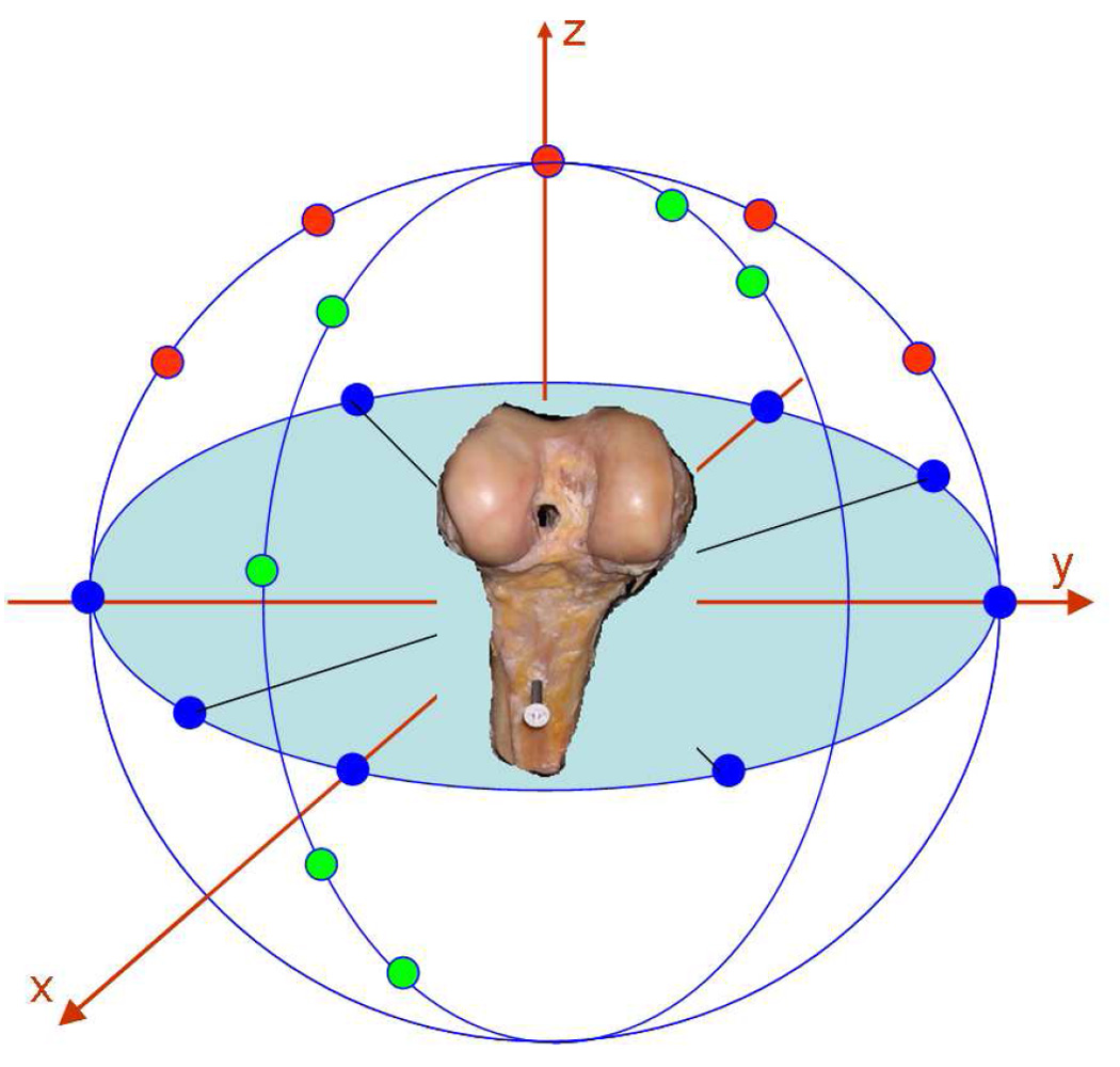
Schematic representation of the laser scanning method. Each bone, with and without articular cartilage, was scanned from twenty different views. Each view is represented as a dot in this figure. The views were then merged to create 3D models, from which a cartilage model was extracted.

Cartilage Thickness

TF cartilage thickness measurements were performed on specific load-bearing ROIs ^{31, 41}. A distinct notch marking the junction between the TF and PF joints on the lateral femoral condyle was identified on the first sagittal MR image in which it appeared [Fig. 2a]. The bone-cartilage interface of the 3D femoral cartilage model was fit with a cylinder [Fig. 2b]. A line was drawn from the notch (0°) to the center of the cylinder. Each femoral condyle was then divided at 40°, 70°, 100°, and 130° from the notch point toward the posterior aspect of the femur to create six femoral ROIs [three medial (M1: 40–70°), (M2: 70–100°), (M3: 100–130°); and three lateral: (L1: 40–70°), (L2: 70–100°), (L3: 100–130°)] [Fig. 2b, c]. Each ROI’s medial-lateral width was 20% of the overall medial-lateral width of the femoral cartilage, and each ROI was centered about the midline of its respective condyle [Fig. 2c].

Figure 2.

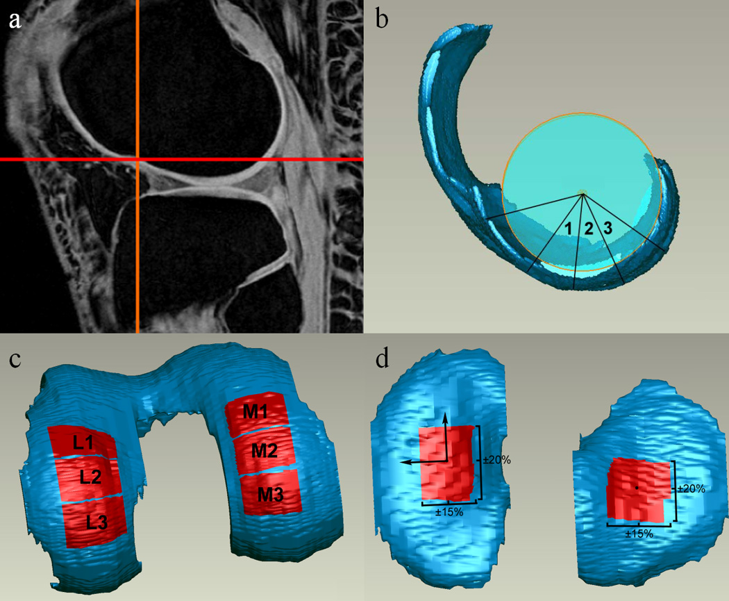
Determination of cartilage regions of interest (ROIs) for thickness measurements. ROIs were selected to represent load-bearing regions of TF articular cartilage. Portions of this figure adapted from a previous manuscript with permission ⁴¹.

Two tibial ROIs [one medial (MT) and one lateral (LT)] were defined on the cartilage regions of the 3D model resulting from segmentation. The centroid of each compartment was calculated with MATLAB (The Mathworks, Inc., Natick MA, USA). The inertial axes of the medial compartment were also determined using MATLAB, and axes of the same orientation were projected onto the centroids of both the medial and lateral tibial compartments. The ROI of each compartment was then defined as the area ±20% of the overall anterior-posterior length and ±15% of the overall medial-lateral width from the centroid [Fig. 2d]. The mean thickness of each cartilage patch was calculated with a closest point algorithm using MATLAB.

The same procedures were used to identify the corresponding ROIs on the tibial and femoral cartilage models obtained from the laser scanning process described above.

Ex vivo Assessment

One fresh-frozen human cadaver knee (54-year-old female) was used to evaluate both the accuracy and reliability of the manual and LiveWire segmentation methods. The specimen showed no evidence of knee injury or cartilage damage upon visual inspection. It was imaged seven times using the T1-weighted WE-3D FLASH sequence. Between each scan, the knee was removed from the coil, flexed and extended twenty times, and reinserted into the coil. The resulting images were segmented and reconstructed using both methods described above. After MR imaging was complete, the joint was disarticulated, and the distal femur and proximal tibia were assessed using the described 3D laser scanning method.

In vivo Assessment

The knee of a healthy volunteer (23-year-old female) was also scanned seven times. Between each scan, the subject exited the scanner, walked around the facility for five minutes, and then re-entered the scanner for the next scan. The MR scans were segmented and reconstructed using both methods described above.

Statistical Analysis

The reliability of each technique (Aim 1) was established by calculating the coefficients of variation (CVs) for the ex vivo and in vivo experiments. To assess the accuracy of both segmentation methods, two-way analyses of variance (factors: method and trials) were performed to compare the mean thickness values of the two segmentation methods with those obtained from the laser scanner, and with each other. Each ROI was analyzed in a separate ANOVA.

Results

Reliability (Aim 1)

The reliability of both segmentation methods was assessed both ex vivo and in vivo by determining the CV(%) for each ROI (M1–3, L1–3, MT, and LT) over the seven repeated MR scans [Table 1]. The cadaver specimen showed mean CVs across all ROIs of 4.16%, 3.02%, and 1.59% for manual segmentation, LiveWire segmentation, and laser scanning, respectively.

Table 1.

Coefficients of variation (%) for each specimen, method, and region of interest.

		Femur						Tibia
Specimen	Method	M1	M2	M3	L1	L2	L3	MT	LT
Cadaver	Manual	4.83	3.35	4.78	3.70	4.41	6.82	2.43	2.93
	LiveWire	3.66	4.72	3.00	2.73	2.16	3.48	2.15	2.23
	Laser	1.00	1.27	2.48	0.75	1.86	1.10	1.52	2.74
Volunteer	Manual	2.89	0.81	1.33	3.74	3.03	3.95	4.23	1.68
	LiveWire	1.59	1.48	5.45	5.80	3.84	6.43	2.54	2.08

In vivo, the mean CVs across all ROIs were 2.71% and 3.65% for manual and LiveWire segmentation, respectively [Table 1].

Accuracy (Aim 2)

The accuracy of both segmentation methods was assessed ex vivo by the comparison of mean ROI thicknesses to laser scanning results [Fig. 3]. The mean absolute error across all ROIs between manual segmentation and laser scanning was 4.07% (5.35% over six femoral ROIs; 0.22% over two tibial ROIs), while this error between LiveWire segmentation and laser scanning was 7.46% (8.93% over six femoral ROIs; 3.06% over two tibial ROIs). With the exception of MT, there were significant differences in thickness values in each ROI measured ex vivo between LiveWire and manual segmentation (p<0.02). Thickness values obtained from LiveWire segmentation consistently underestimated those obtained by manual segmentation and laser scanning [Fig. 3]. The region MT showed no significant differences between manual segmentation, LiveWire segmentation, or laser scanning (p=0.11). The regions M1, M2, and L1 showed significant differences in thickness measurements between LiveWire segmentation and laser scanning (p<0.001), whereas regions M3, L2, L3, and LT did not (p>0.08). Similarly, the regions M2, M3, and L2 showed significant differences in thickness measurements between manual segmentation and laser scanning (p<0.025), whereas regions M1, L1, L3, and LT did not (p>0.11).

Figure 3.

Ex vivo mean cartilage thickness values (mm) for (a) femoral and (b) tibial regions of interest (ROIs) assessed with each technique. Significant differences between laser scanning and manual segmentation, and between laser scanning and LiveWire, are denoted with * (p<0.05) and # (p<0.01). Significant differences between LiveWire and manual segmentation are not shown.

In vivo, each ROI over seven trials showed significantly different thickness measurements between the two segmentation methods (p<0.011). LiveWire segmentation consistently underestimated manual segmentation. When pooled across the femoral ROIs, manual and LiveWire segmentations produced mean thickness values of 2.33(±0.024)mm and 2.04(±0.034)mm, respectively. Similarly, when pooled across the tibial ROIs, the manual and LiveWire segmentations produced mean values of 2.81(±0.061)mm and 2.47(±0.041)mm, respectively.

Discussion

Both the LiveWire and manual segmentation techniques were repeatable for analyzing TF articular cartilage thickness. The segmentation-based thickness measurements each had mean CVs of less than 4.17%, both ex vivo and in vivo, in the defined ROIs over seven trials (Aim 1). Similarly, laser scanning thickness measurements had a mean CV of 1.59% over seven trials, suggesting that this method is an acceptable gold standard for the evaluation of segmentation-based cartilage thickness measurements. In vivo, the mean CVs across all ROIs were 2.71% and 3.65% for manual and LiveWire segmentation, respectively. When the accuracy of each segmentation technique was assessed, the mean absolute error between manual segmentation and laser scanning was 4.07% (5.35% over the femoral ROIs; 0.22% over the tibial ROIs), while the mean absolute error between LiveWire segmentation and laser scanning was 7.46% (8.93% over the femoral ROIs; 3.06% over the tibial ROIs) (Aim 2). These results indicate that although each method is repeatable, TF cartilage thickness measurements based upon manual segmentation more closely approximate true cartilage thicknesses than do those based upon LiveWire segmentation.

While there are several possible explanations for the generally lower CVs seen in vivo, it is likely that a living knee has higher water content than does a cadaver knee, and therefore provides greater articular cartilage contrast on MRI. Differences in age and tissue fixation between the cadaveric and living specimens may also explain the noted results. Similarly, there are several possible explanations for the much lower absolute errors seen in the tibial ROIs when compared to the femoral ROIs. The femoral cartilage is curved, and therefore is not consistently orthogonal to the long axis of the magnetic field when compared to the relatively flat tibia. The curved femoral cartilage is prone to more error due to partial volume effects, as well as other MRI and voxel reconstruction phenomena. In addition, tibial cartilage, in both compartments, is generally thicker than femoral cartilage. Because the mean tibial thickness is greater, the error value will translate to a smaller percent error than in the femur. When combined, these explanations may account for the lower absolute errors seen in the tibia.

LiveWire thickness measurements consistently underestimated those made with manual segmentation and laser scanning. This underestimation suggests a systematic error in the calculation of cartilage thickness with LiveWire. It is feasible, therefore, that this error may be reduced by systematically adjusting the cartilage thickness values obtained from LiveWire segmentation, thereby improving the accuracy of LiveWire-based cartilage thickness measurements. There are many possible explanations for this segmentation bias; one is that each method uses a slightly different interpolation algorithm when creating segmentation-based 3D models. Second, the process of reconstructing a 3D model from LiveWire segmentation requires several steps of manual user input, including the repair of any errors associated with the “wrapping” of the triangular mesh, and therefore allows some room for variability. The 3D model reconstruction process associated with manual segmentation, however, is automated. Therefore, the source of error may be in the reconstruction process, rather than in segmentation. Although this represents a limitation of the LiveWire method in its current form, its 3D modeling process could be adjusted and streamlined in the future.

Despite the apparently systematic error associated with LiveWire, the method has several inherent advantages over manual segmentation. LiveWire segmentation is faster than manual segmentation, which is tedious and time-consuming; manual segmentation of one set of images may take up to two hours. Because LiveWire employs an algorithm with smaller bounding boxes than traditional semi-automated segmentation techniques, it is less likely to become trapped in local minima. As previously mentioned, LiveWire was programmed for our purposes to work in concert with manual segmentation when a local defect was encountered in which the segmentation was not clear. This feature was employed only when LiveWire could not find an appropriate boundary. Thus, the option to switch to manual segmentation when necessary allowed the user to capture features of the articular cartilage that the primary semi-automated segmentation approach might have excluded, while still decreasing segmentation time. Although it is not certain whether this feature would be an advantage for segmenting of knees with generalized chondral defects, we would hypothesize that the addition of the manual segmentation option to the semi-automated algorithm would remain an advantage for such knees, especially since these knees are often more challenging to segment than healthy knees.

After examining the results of the present study, we qualitatively evaluated the differences between manual and LiveWire segmentation by overlaying representative contours of each method onto their respective MR image slices. We saw that while LiveWire seemed to more closely approximate cartilage boundaries toward the extreme edges of the tibial and femoral cartilage, manual segmentation appeared to provide a closer approximation in regions of low contrast and cartilage contact. Manual segmentation results may have appeared more favorable in the present study because the ROIs examined were focused upon load-bearing cartilage areas, rather than the edges of the cartilage structures. Additionally, it may be possible that the differences in thickness seen in the varying weight-bearing regions may have been due simply to the fact that some regions have greater average thickness values than others. In regions with greater average thickness, such as L2 and LT, a small difference in thickness between segmentation methods, although valid, may not be statistically significant, because the percent difference is relatively small. Similarly, in regions with small average thickness values, such as M1 and L1, a small difference in thickness may be statistically significant because the percent difference is relatively large. Because LiveWire appears to be more effective in some areas of the knee joint, while manual segmentation is better in others, some efficient combination of both methods, similar to the program employed in this study, may provide the best results while still offering decreased segmentation time.

The ROIs examined in the present study were chosen to represent the weight-bearing regions of the femur and tibia. Because qMRI is useful for tracking the onset and progression of early OA, it seems practical to focus on thickness changes in weight-bearing regions.

A “fully” automated segmentation technique has recently been reported ^{13, 28, 43}. This method, however, requires the use of manual segmentation to “teach” the software to properly segment cartilage. These methods have, thus far, only been applied to healthy joints; their success on joints with varying degrees of OA progression remains unknown, and the evaluations have only been performed using low-field (0.18T) MRI.

In 2005, Koo et al. published a study evaluating knee cartilage thickness with segmented MR images ³¹. In that study, Koo et al. used a semi-automated B-Spline snake segmentation method to measure cartilage thickness in six femoral ROIs ex vivo and in vivo. The ex vivo specimens were porcine, and were evaluated with both MRI segmentation and 3D laser scanning, similar to the evaluation described in the present study. Koo et al. reported in vivo intra-observer femoral thickness measurement CVs of 2–3%, which are comparable to the values reported in the current study. For one in vivo specimen that was scanned twice, Koo reported variability of approximately 4% of the total cartilage thickness in weight-bearing regions. Although the ROIs defined by Koo et al. were slightly different than those described in the present study, the results were comparable in terms of accuracy and reliability. Although Koo et al. reported some tibial thickness data, the details concerning these measurements were not specified.

The present study has some limitations. The accuracy assessment (Aim 2) of MR imaging-based cartilage thickness measurements assumes that laser scanning is the gold standard. A preliminary validation study showed laser scanning thickness measurements of phantom articular cartilage to be within 4.5% and 3.6% of caliper-based thickness measurements for the femoral and tibial cartilage, respectively. Although it is difficult to determine the true cartilage thickness of a cadaver specimen, our laser scanning method showed a mean CV of 1.59% for all ROIs over seven trials, indicating that the method was reliable. The use of laser scanning also prevented the assessment of accuracy in vivo, a problem that was offset in the present study by the addition of an ex vivo component. Additionally, the ex vivo MR images used within this study were not affected by motion or blood flow artifacts; for this reason, we also tested both segmentation methods in vivo. Finally, due largely to the amount of time required for acquiring and processing the laser scan data, this study includes a limited number of samples (two knees—one cadaver, one volunteer—each scanned seven times). Even with this number of samples, however, we were able to detect statistically significant differences in articular cartilage thickness measurements between methods. It is important to note that the purpose of this study was to compare the reliability of two separate methods of articular cartilage segmentation; therefore, knees of different stages of OA, focal and generalized chondral defects, and different ages and genders were not evaluated. The ex vivo and in vivo specimens scanned multiple times allowed for evaluation of variability due to each segmentation method, without the complication of examining knees in various conditions.

In conclusion, manual segmentation, LiveWire segmentation, and laser scanning are repeatable methods for quantifying tibiofemoral articular cartilage thickness. However, the thickness measurements appear to be technique-dependent. Assuming that the laser scanning method is an appropriate standard for comparison, manual segmentation provided a more accurate measurement of cartilage thickness in load-bearing regions of the tibiofemoral joint.

References

- 1.Cicuttini FM, Wluka AE, Stuckey SL. Tibial and femoral cartilage changes in knee osteoarthritis. Ann Rheum Dis. 2001;60:977–980. doi: 10.1136/ard.60.10.977. [DOI] [PMC free article] [PubMed] [Google Scholar]
- 2.Eckstein F, Burstein D, Link TM. Quantitative MRI of cartilage and bone: degenerative changes in osteoarthritis. NMR Biomed. 2006;19:822–854. doi: 10.1002/nbm.1063. [DOI] [PubMed] [Google Scholar]
- 3.Amin S, LaValley MP, Guermazi A, Grigoryan M, Hunter DJ, Clancy M, et al. The relationship between cartilage loss on magnetic resonance imaging and radiographic progression in men and women with knee osteoarthritis. Arthritis Rheum. 2005;52:3152–3159. doi: 10.1002/art.21296. [DOI] [PubMed] [Google Scholar]
- 4.Jones G, Ding CH, Scott F, Glisson M, Cicuttini F. Early radiographic osteoarthritis is associated with substantial changes in cartilage volume and tibial bone surface area in both males and females. Osteoarthritis Cartilage. 2004;12:169–174. doi: 10.1016/j.joca.2003.08.010. [DOI] [PubMed] [Google Scholar]
- 5.Graichen H, von Eisenhart-Rothe R, Vogl T, Englmeier KH, Eckstein F. Quantitative assessment of cartilage status in osteoarthritis by quantitative magnetic resonance imaging: technical validation for use in analysis of cartilage volume and further morphologic parameters. Arthritis Rheum. 2004;50:811–816. doi: 10.1002/art.20191. [DOI] [PubMed] [Google Scholar]
- 6.Cicuttini F, Wluka A, Hankin J, Wang Y. Longitudinal study of the relationship between knee angle and tibiofemoral cartilage volume in subjects with knee osteoarthritis. Rheumatology. 2004;43:321–324. doi: 10.1093/rheumatology/keh017. [DOI] [PubMed] [Google Scholar]
- 7.Raynauld JP, Martel-Pelletier J, Berthiaume MJ, Labonte F, Beaudoin G, de Guise JA, et al. Quantitative magnetic resonance imaging evaluation of knee osteoarthritis progression over two years and correlation with clinical symptoms and radiologic changes. Arthritis Rheum. 2004;50:476–487. doi: 10.1002/art.20000. [DOI] [PubMed] [Google Scholar]
- 8.Cicuttini FM, Wluka AE, Wang Y, Stuckey SL. Longitudinal study of changes in tibial and femoral cartilage in knee osteoarthritis. Arthritis Rheum. 2004;50:94–97. doi: 10.1002/art.11483. [DOI] [PubMed] [Google Scholar]
- 9.Raynauld JP, Kauffmann C, Beaudoin G, Berthiaume MJ, de Guise JA, Bloch DA, et al. Reliability of a quantification imaging system using magnetic resonance images to measure cartilage thickness and volume in human normal and osteoarthritic knees. Osteoarthritis Cartilage. 2003;11:351–360. doi: 10.1016/s1063-4584(03)00029-3. [DOI] [PubMed] [Google Scholar]
- 10.Glaser C, Burgkart R, Kutschera A, Englmeier KH, Reiser M, Eckstein F. Femoro-tibial cartilage metrics from coronal MR image data: Technique, test-retest reproducibility, and findings in osteoarthritis. Magn Reson Med. 2003;50:1229–1236. doi: 10.1002/mrm.10648. [DOI] [PubMed] [Google Scholar]
- 11.Biswal S, Hastie T, Andriacchi TP, Bergman GA, Dillingham MF, Lang P. Risk factors for progressive cartilage loss in the knee: a longitudinal magnetic resonance imaging study in forty-three patients. Arthritis Rheum. 2002;46:2884–2892. doi: 10.1002/art.10573. [DOI] [PubMed] [Google Scholar]
- 12.Wluka AE, Stuckey S, Snaddon J, Cicuttini FM. The determinants of change in tibial cartilage volume in osteoarthritic knees. Arthritis Rheum. 2002;46:2065–2072. doi: 10.1002/art.10460. [DOI] [PubMed] [Google Scholar]
- 13.Qazi AA, Folkesson J, Pettersen PC, Karsdal MA, Christiansen C, Dam EB. Separation of healthy and early osteoarthritis by automatic quantification of cartilage homogeneity. Osteoarthritis Cartilage. 2007;15:1199–1206. doi: 10.1016/j.joca.2007.03.016. [DOI] [PubMed] [Google Scholar]
- 14.Bauer J, Krause S, Ross C, Krug R, Carballido-Gamio J, Ozhinsky E, et al. Volumetric Cartilage Measurements of Porcine Knee at 1.5-T and 3.0-T MR Imaging: Evaluation of Precision and Accuracy. Radiology. 2006;241:399–406. doi: 10.1148/radiol.2412051330. [DOI] [PubMed] [Google Scholar]
- 15.Bolbos R, Benoit_cattin H, Langlois J-B, Chomel A, Chereul E, Odet C, et al. Knee cartilage thickness measurements using MRI: a 4 1/2-month longitudinal study in the meniscectomized guinea pig model of OA. Osteoarthritis Cartilage. 2007;15:656–665. doi: 10.1016/j.joca.2006.12.009. [DOI] [PubMed] [Google Scholar]
- 16.Bolbos R, Benoit-cattin H, Langlois JB, Chomel A, Chereul E, Odet C, et al. Measurement of knee cartilage thickness using MRI: a reproducibility study in a meniscectomized guinea pig model of osteoarthritis. NMR in Biomed. 2007 doi: 10.1002/nbm.1198. [DOI] [PubMed] [Google Scholar]
- 17.Eckstein F, Schnier M, Haubner M, Priebsch J, Glaser C, Englmeier KH, et al. Accuracy of cartilage volume and thickness measurements with magnetic resonance imaging. Clin Orthop. 1998;352:137–148. [PubMed] [Google Scholar]
- 18.Solloway S, Hutchinson CE, Waterton JC, Taylor CJ. The use of active shape models for making thickness measurements of articular cartilage from MR images. Magn Reson Med. 1997;37:943–952. doi: 10.1002/mrm.1910370620. [DOI] [PubMed] [Google Scholar]
- 19.Kshirsagar AA, Watson PJ, Tyler JA, Hall LD. Measurement of localized cartilage volume and thickness of human knee joints by computer analysis of three-dimensional magnetic resonance images. Invest Radiol. 1998;33:289–299. doi: 10.1097/00004424-199805000-00006. [DOI] [PubMed] [Google Scholar]
- 20.Kauffmann C, Gravel P, Godbout B, Gravel A, Beaudoin G, Raynauld JP, et al. Computer-aided method for quantification of cartilage thickness and volume changes using MRI: Validation method using a synthetic model. IEEE Trans Biomed Engin. 2003;50:978–988. doi: 10.1109/TBME.2003.814539. [DOI] [PubMed] [Google Scholar]
- 21.Stammberger T, Eckstein F, Michaelis M, Englmeier KH, Reiser M. Interobserver reproducibility of quantitative cartilage measurements: comparison of B-spline snakes and manual segmentation. Magn Reson Imag. 1999;17:1033–1042. doi: 10.1016/s0730-725x(99)00040-5. [DOI] [PubMed] [Google Scholar]
- 22.Stammberger T, Eckstein F, Englmeier KH, Reiser M. Determination of 3D cartilage thickness data from MR imaging: computational method and reproducibility in the living. Magn Reson Med. 1999;41:529–536. doi: 10.1002/(sici)1522-2594(199903)41:3<529::aid-mrm15>3.0.co;2-z. [DOI] [PubMed] [Google Scholar]
- 23.Gougoutas AJ, Wheaton AJ, Borthakur A, Shapiro EM, Kneeland JB, Udupa JK, et al. Cartilage volume quantification via Live Wire segmentation. Acad Radiol. 2004;11:1389–1395. doi: 10.1016/j.acra.2004.09.003. [DOI] [PubMed] [Google Scholar]
- 24.Eckstein F, Kunz M, Schutzer M, Hudelmaier M, Jackson RD, Yu J, et al. Brief report: Two year longitudinal change and test--retest-precision of knee cartilage morphology in a pilot study for the osteoarthritis initiative. Osteoarthritis Cartilage. 2007;15:1326–1332. doi: 10.1016/j.joca.2007.04.007. [DOI] [PMC free article] [PubMed] [Google Scholar]
- 25.Eckstein F, Buck RJ, Wyman BT, Kotyk JJ, Hellio Le Graverand MP, Remmers AE, et al. Quantitative Imaging of Cartilage Morphology at 3.0 Tesla in the Presence of Gadopentate Dimeglumine (Gd-DTPA) Magn Reson Med. 2007;58:402–406. doi: 10.1002/mrm.21290. [DOI] [PubMed] [Google Scholar]
- 26.Eckstein F, Kunz M, Hudelmaier M, Jackson R, Yu J, Eaton CB, et al. Impact of Coil Design on the Contrast-to-Noise Ratio, Precision, and Consistency of Quantitative Cartilage Morphology at 3 Tesla: A Pilot Study for the Osteoarthritis Initiative. Magn Reson Med. 2007;57:448–454. doi: 10.1002/mrm.21146. [DOI] [PubMed] [Google Scholar]
- 27.Inglis D, Pui M, Ioannidis G, Beattie K, Boulos P, Adachi JD, et al. Brief report: Accuracy and test-retest precision of quantitative cartilage morphology on a 1.0T peripheral magnetic resonance imaging system. Osteoarthritis Cartilage. 2007;15:110–115. doi: 10.1016/j.joca.2006.08.006. [DOI] [PubMed] [Google Scholar]
- 28.Folkesson J, Dam EB, Olsen OF, Pettersen PC, Christiansen C. Segmenting articular cartilage automatically using a voxel classification approach. IEEE Trans Med Imag. 2007;26:106–115. doi: 10.1109/TMI.2006.886808. [DOI] [PubMed] [Google Scholar]
- 29.Potter HG, Foo LF. Magnetic Resonance Imaging of Articular Cartilage. Am J Sports Med. 2006;34:661–677. doi: 10.1177/0363546505281938. [DOI] [PubMed] [Google Scholar]
- 30.Hargreaves BA, Gold GE, Beaulieu CF, Vasanawala SS, Nishimura DG, Pauly JM. Comparison of New Sequences for High-Resolution Cartilage Imaging. Magn Reson Med. 2003;49:700–709. doi: 10.1002/mrm.10424. [DOI] [PubMed] [Google Scholar]
- 31.Koo S, Gold GE, Andriacchi TP. Considerations in measuring cartilage thickness using MRI: factors influencing reproducibility and accuracy. Osteoarthritis Cartilage. 2005;13:782–789. doi: 10.1016/j.joca.2005.04.013. [DOI] [PubMed] [Google Scholar]
- 32.Kass M, Witkin A, Terzopoulos D. Snakes: Active contour models. Int J Computer Vis. 1987;1:321–331. [Google Scholar]
- 33.Tek H, Kimia BB. Volumetric segmentation of medical images by three-dimensional bubbles. Computer Vision Imag Understanding. 1997;65:246–258. [Google Scholar]
- 34.Amini AA, Weymouth TE, Jain RC. Using dynamic programming for solving variational problems in vision. IEEE Trans Pattern Analysis Machine Intelligence. 1990;12:855–867. [Google Scholar]
- 35.Sebastian TB, Tek H, Crisco JJ, Kimia BB. Segmentation of carpal bones from CT images using skeletally coupled deformable models. Med Imag Analysis. 2003;7:21–45. doi: 10.1016/s1361-8415(02)00065-8. [DOI] [PubMed] [Google Scholar]
- 36.Barrett WA, Mortensen EN. Interactive Live-Wire Boundary Extraction. Med Imag Analysis. 1997;1:331–341. doi: 10.1016/s1361-8415(97)85005-0. [DOI] [PubMed] [Google Scholar]
- 37.Falcao AX, Udupa JK, Miyazawa FK. An ultra-fast user-steered image segmentation paradigm: live wire on the fly. IEEE Trans Med Imag. 2000;19:55–62. doi: 10.1109/42.832960. [DOI] [PubMed] [Google Scholar]
- 38.Song Y, Greve JM, Carter DR, Koo S, Giori NJ. Articular cartilage MR imaging and thickness mapping of a loaded knee joint before and after meniscectomy. Osteoarthritis Cartilage. 2006;14:728–737. doi: 10.1016/j.joca.2006.01.011. [DOI] [PubMed] [Google Scholar]
- 39.Wluka AE, Wolfe R, Stuckey S, Cicuttini FM. How does tibial cartilage volume relate to symptoms in subjects with knee osteoarthritis? Ann Rheum Dis. 2004;63:264–268. doi: 10.1136/ard/2003.007666. [DOI] [PMC free article] [PubMed] [Google Scholar]
- 40.Li G, DeFrate LE, Park SE, Gill TJ, Rubash HE. In vivo articular cartilage contact kinematics of the knee: an investigation using dual-orthogonal fluoroscopy and magnetic resonance image-based computer models. Am J Sports Med. 2005;33:102–107. doi: 10.1177/0363546504265577. [DOI] [PubMed] [Google Scholar]
- 41.Bowers ME, Tung GA, Trinh N, Leventhal E, Crisco JJ, Kimia B, et al. Effects of ACL interference screws on articular cartilage volume and thickness measurements with 1.5 T and 3 T MRI. Osteoarthritis Cartilage. 2007 doi: 10.1016/j.joca.2007.09.010. [DOI] [PMC free article] [PubMed] [Google Scholar]
- 42.Chang MC, Leymarie FF, Kimia BB. Surface Reconstruction from Point Clouds by Transforming the Medial Scaffold. 3-D Digital Imaging and Modeling (3DIM) 2007:13–20. [Google Scholar]
- 43.Folkesson J, Dam EB, Olsen OF, Christiansen C. Accuracy evaluation of automatic quantification of the articular cartilage surface curvature from MRI. Acad Radiol. 2007;14:1221–1228. doi: 10.1016/j.acra.2007.07.001. [DOI] [PubMed] [Google Scholar]