

Abstract
We have developed a method and a device entitled prostate mechanical imager (PMI) for the real-time imaging of prostate using a transrectal probe equipped with a pressure sensor array and position tracking sensor. PMI operation is based on measurement of the stress pattern on the rectal wall when the probe is pressed against the prostate. Temporal and spatial changes in the stress pattern provide information on the elastic structure of the gland and allow two-dimensional (2-D) and three-dimensional (3-D) reconstruction of prostate anatomy and assessment of prostate mechanical properties. The data acquired allow the calculation of prostate features such as size, shape, nodularity, consistency/hardness, and mobility. The PMI prototype has been validated in laboratory experiments on prostate phantoms and in a clinical study. The results obtained on model systems and in vivo images from patients prove that PMI has potential to become a diagnostic tool that could largely supplant DRE through its higher sensitivity, quantitative record storage, ease-of-use and inherent low cost.
Index Terms: Elastography, mechanical imaging, prostate, prostate cancer screening, tissue elasticity
I. Introduction
Prostate cancer is one of the most common causes of death from cancer in the United States. The American Cancer Society estimates that in 2005, approximately 232 090 new cases of prostate cancer will be diagnosed in the United States alone, and 30 350 men will die of the disease [1]. Current methods of prostate assessment include digital rectal examination (DRE), prostate specific antigen (PSA) blood test, transrectal ultrasound (TRUS), computerized axial scanning tomography (CT), and endorectal magnetic resonance imaging (MRI). During DRE, a health professional inserts a lubricated, gloved finger of one hand into the rectum to check for abnormalities of the prostate. Both CT and MRI are not widely accepted by urologists because of lack of proper training, complexity of examination and costs associated with these tests. The most commonly employed screening techniques remain DRE and PSA, while TRUS or TRUS-guided biopsy are considered main tools for advanced prostate cancer diagnostics. Although TRUS-guided biopsy is currently the standard for detecting prostate cancer in the United States, TRUS cannot distinguish reliably between cancerous and noncancerous tissue [2].
Screening for prostate cancer remains a controversial issue due to many apparent limitations in both DRE and PSA. Effectiveness of DRE is limited by the fact that the test is highly subjective depending on examiners training, experience, and ability to interpret the results. An overview of studies of screening suggests that DRE alone detects less than 60% of prevalent prostate cancers [3], while a meta-analysis of DRE as screening test reveals overall sensitivity, specificity, and positive predictive value at 53.2%, 83.6%, and 17.8%, respectively [4]. Sensitivity and specificity of PSA screening is also questionable. Specificity of a cut-point of 4.0 ng/ml has been estimated at around 90% on the first screening round but declines with increasing age and the presence of benign prostatic hypertrophy (BPH) [3], [5]. The sensitivity, specificity, and positive predictive value of PSA were reported at 72.1%, 93.2%, and 25.1%, respectively [4]. Despite evident drawbacks of both methods, the combination of DRE and PSA do appear to increase the yield of screening; in a large study of volunteers, 26% more cancers were detected than PSA alone [6]. Therefore, a method that mimics DRE, but with enhanced sensitivity and specificity, might consequently lead to a greater screening yield. Such a method for visualizing the prostate structure and assessing its mechanical properties with sensitivity exceeding that of manual palpation is described in this paper. The method termed mechanical imaging (MI) translates the tissue’s elastic properties into a digital three-dimensional (3-D) map of the tested organ [7]. MI is based on reconstructing the internal structure of soft tissues using the data obtained by a force sensor array pressed against the examined site. The changes in the surface stress patterns as a function of displacement, pressure, and time provide information regarding elastic composition and geometry of the organ.
MI is a branch of Elastography—an emerging medical imaging technology. Various versions of ultrasound elastography (USE) and magnetic resonance elastography (MRE) have been developed during last decade [8]-[19] and tested in a broad range of clinical applications including prostate cancer detection [20]-[27]. USE and MRE are based on visualization of changes in the strain pattern in the tissue under various types of loading. In contrast to USE and MRE, MI is based on measurements of surface stress patterns which are related to the internal strain patterns and spatial distribution of tissue elasticity.
Evaluation of tissue “hardness” (shear elasticity modulus) by various elasticity imaging techniques provides a means for characterizing the tissue, differentiating normal and diseased conditions, and detecting tumors and other lesions [10], [28], [29]. Measurements on excised prostate specimens showed the normal prostate tissue has a modulus that is lower than the modulus of the prostate cancers, while the tissue from prostate with benign prostatic hyperplasia had modulus values significantly lower than normal tissue [28]. Tumor inclusions or tissue blocked from its blood nutrients are stiffer than normal tissue; benign and cancerous tumors also have distinguishing elastic properties.
In one of the earliest USE studies conducted on prostatectomy specimens, it was shown that elasticity imaging is more sensitive for tumor detection and more accurate for assessment of tumor location than was conventional ultrasonography [20]. Sixty-four percent of pathologically confirmed tumors detected at elasticity imaging were isoechoic on conventional ultrasound images. Comparative in vivo studies of efficiency of prostate cancer diagnostics using USE versus conventional ultrasound imaging showed a significant improvement in the detection rate of prostatic cancer [22], [23], [26]. Elastography detected additional five cancers in 100 patients [23]. It was shown that USE allows an accurate measurement of tumor size and localization in contrast to conventional transrectal ultrasound and may be very useful and efficient in biopsy guidance for prostate cancer detection [22], [26]. Elastography images clearly show malignant tissue areas, which are inconspicuous in the B-mode ultrasound image [26].
In the studies on feasibility of in vivo MRE of the prostate, highly accurate reconstruction of distribution of elasticity inside the gland correlating with the zonal anatomy of the prostate has been achieved [25]. The accuracy of elasticity modulus evaluation was estimated to be better than 1 kPa, while as it is known from the literature, the difference of moduli of normal and cancerous prostate tissue may exceed tens and even hundreds of kPa [28], [29].
Since elasticity modulus of soft tissues may greatly change in the course of the pathological and physiological processes, elastography has a potential for monitoring therapeutic procedures. The ability of USE to monitor high-intensity focused ultrasound (HIFU) prostate cancer treatment has been evaluated [24], [27]. Using a comparison with magnetic resonance imaging, it was shown that an ultrasonic elastography imaging system that may provide a simple and cost-effective solution to monitor HIFU treatments [27].
The data accumulated in the last decade clearly shows great potential of elastographic methods in the detection of prostate cancer, as well as in the biopsy guidance and treatment monitoring. The proven ability of Elastography to distinguish benign and cancerous tissue is reason for greatly increasing activity word wide in developing various versions of the technology. MI, which is being developed at Artann Laboratories, Trenton, NJ, during last 10 years, yields 3-D map of tissue elasticity, similar to other elastographic techniques. At the same time, the MI is most closely mimicking manual palpation since the MI transrectal probe with a pressure sensor array mounted on its tip acts similar to a human finger during DRE, slightly compressing the prostate by the probe. In essence, MI “captures the sense of touch” and stores it permanently in digital format for later prostate analysis and comparison. Extensive laboratory studies on prostate phantoms and excised prostates have shown that the computerized palpation is more sensitive than human finger [30]-[33]. Currently, the frequency with which DRE is performed and the quality of DRE is inadequate because of low efficiency of the procedure, insufficient training, and absence of confidence of the examiners [34], [35].
The main purpose of this study was the development and validation of the prostate mechanical imager (PMI), a device for real-time imaging of the prostate and assessment of prostate features such as size, shape, consistency/hardness, mobility, and nodularity. The PMI prototype has been validated in a clinical study and the results of the study show that PMI has potential to become a diagnostic and cancer screening tool that could largely supplant DRE through its higher sensitivity, quantitative record storage, ease-of-use, portability, minimal training required, and inherent low cost.
II. Prostate Mechanical Imaging System
A. System Overview
The PMI includes a transrectal probe, an electronic unit, and a laptop computer with data acquisition card. The transrectal probe comprises two separate pressure sensor arrays and orientation sensors, as shown in Fig. 1. The first pressure sensor array is installed on the probe head surface contacting with prostate through the rectal wall during examination procedure. The probe head is shifted down relative to the probe shaft with 8° inclination and measures 50 mm in length, 18 mm in width, and 12.7 mm in height having ellipsoidal cross section. The probe head pressure sensor array comprises 128 (16 × 8) pressure sensors covering 40 mm × 16 mm. Each pressure sensor [36] has rectangular pressure sensing area 2.5 mm by 2.0 mm (Pressure Profile Systems, CA). Each sensor has sensitivity of about 0.05 kPa and hysteresis of 2%–4% of the operational range. The second pressure sensor array is installed on the probe shaft surface for assessment of the pressure pattern in the sphincter area during prostate examination. The probe shaft measures 65 mm in length and 12.7 mm in diameter. The shaft pressure array is different from that of the probe head. It comprises the same number of sensors (16 × 8) but the sensors have different dimensions (3.75 mm × 2.5 mm). Ultrasound FDA approved probe cover #40500 (Sheathing Technology, Morgan Hill, CA), 44 μm thickness, was selected as disposable cover for the use with the probe. This elastic cover has mechanical properties which do not influence the stress pattern measured by the probe for model objects having mechanical characteristics close to the real prostate. The cover protects the entire surface of the probe head, the probe shaft, and half of the probe handle.
Fig. 1.
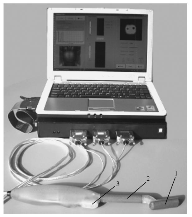
General view of PMI. Transrectal probe of the PMI comprises 1) probe head pressure sensor array for prostate imaging, 2) probe shaft pressure sensor array for sphincter imaging, and 3) probe orientation sensors.
The probe orientation system is composed of three-axis magnetic sensor HMC1023 (Honeywell International, Morristown, NJ) and two-axis acceleration sensor ADXL202 (Analog Devices, Willmington, MA). Both microsensors are placed on a compact platform (20 mm × 9 mm) incorporated inside the probe handle to be in the vicinity of the sphincter during prostate examination (see Fig. 1). The magnetic sensor readings provide azimuth orientation relative to earth’s magnetic field. To compensate the magnetic sensor reading for a platform tilt relative to a horizontal plane, which is perpendicular to earth’s gravity vector, we need to know the platform tilt angles which are measured by two-axis accelerometer used as a tilt sensor to provide elevation and rotation readings. Similar 3-D orientation systems are often used in navigational [37] and virtual reality devices [38].
The electronic unit includes a standard pressure sensor electronics manufactured by Pressure Profile Systems, Inc. (Los Angeles, CA) operating with 256 sensors and communicating with a laptop computer through a USB port, and Artann’s custom designed printed circuit board with orientation sensor amplifiers and magnetic sensors set/reset pulse circuit. PCMCIA data acquisition card DAQCard-6024E (National Instruments Corporation, TX) is employed for orientation data transfer to the laptop computer (Inspiron, Dell, TX) with Pentium M processor 725 (2.0 GHz/400 MHz FSB). PMI data acquisition rate is about 20 frames per second.
Fig. 2 represents an operational diagram of PMI. The probe head pressure sensors are intended for acquisition prostate pressure patterns as well as for calculation of the possible prostate displacements during probe head pressing against the prostate. The probe shaft pressure sensors provide capturing and tracking for the sphincter position allowing real-time spatial visualization of the sphincter and prostate area to help an operator in finding the prostate and assist in probe manipulation. Another important function of the probe shaft sensor array is to provide quantitative information on the level of forces exerted by the operator on the sphincter. Displaying this information on the user interface helps the operator to avoid excessive stretching of patient’s sphincter, which is one of the causes of patient’s discomfort during examination. Calculated distance between the sphincter and prostate and the probe azimuth angle help to compute left/right probe head displacement relative to a start reference line.
Fig. 2.
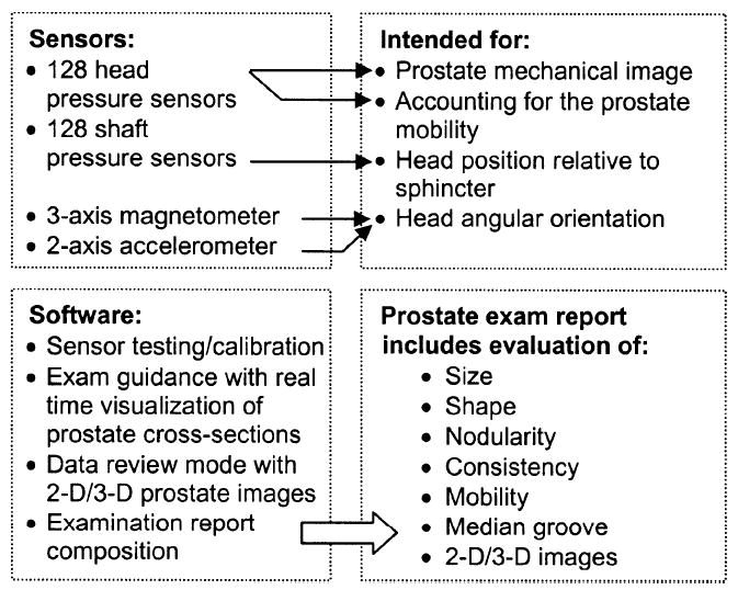
PMI operation diagram.
PMI provides three operational modes: examination procedure, data management, and device management mode. The software allows real-time visualization as well as two-dimensional (2-D)/3-D reconstruction of the prostate, visualization of sphincter and prostate area by means of two orthogonal prostate cross sections generated by integration of sensor pressure readings from the entire palpated region with the relative probe head position. User interface comprises also data management tab allowing data storing and retrieval, as well as printout of the summary report to store in a patient’s chart. Device management tab is utilized for software configuration and probe identification. Basic procedures, which we implemented in the device, are listed in the left lower frame in Fig. 2. The user interface for the examination mode is shown in Fig. 3.
Fig. 3.
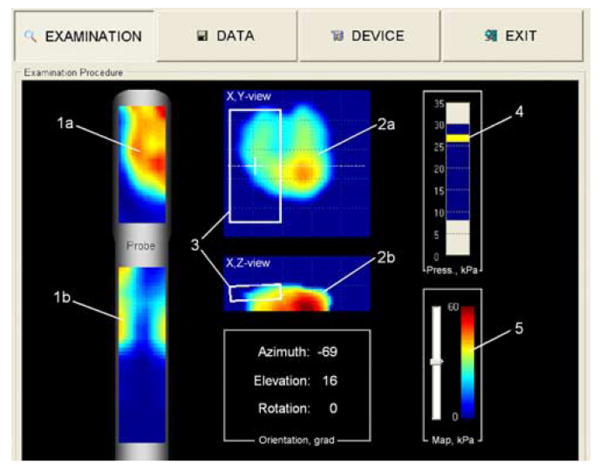
Prostate examination interface. (1a) Momentary prostate pressure pattern. (1b) Sphincter pressure pattern. (2a) Real-time composed frontal and (2b) transversal cross sections of the prostate. (3) Momentary position and orientation of the probe sensors relative to the prostate. (4) Indicator of total applied force to the probe head. (5) Stress level color-bar. (Color version available online at http://ieeexplore.ieee.org.)
B. Examination Procedure
The examination is performed in the standing position, by bending the patient over the examination table to form a 90° angle at the waist. The patient’ chest is placed on the table and the patient’s weight is applied to the table surface so that leg muscles are free from any tension. The probe is covered with a disposable lubricated cover. During the insertion into the rectum, pressure applied to the anal sphincter should be monitored in order to minimize the level of patient’s discomfort. Pressure response data obtained from the supplemental shaft sensor array may be used for that purpose. Gentle posterior pressure is applied as the probe is slowly inserted with the probe head sensor surface down. Allowing a few seconds for the external and internal sphincter to relax will avoid patient discomfort. Scanning begins by first imaging the sphincter used as a supplemental reference organ. Then, the probe is inserted deeper until the bladder is visualized at the very tip of the probe. Next, by sliding the probe backwards, the prostate is detected at about 4–5 cm from the sphincter and the probe is positioned in a way that enables the device to display the prostate gland surface in the center of the screen. Once the probe is properly positioned, an examiner presses a start button on the probe handle to initialize prostate image composition procedure. The prostate scan is performed through a set of multiple pressings on the median groove and lateral lobes of the prostate. Each location of compression of the prostate is selected such that it overlaps with the previous one. The examiner sees in real-time two orthogonal prostate cross sections (Fig. 3) with relative location of the probe head pressure sensitive area in both projections. In certain cases, change in the elevation angle of the probe is required to visualize the prostate. The total prostate scan takes 40–60 s and collected data are instantly saved in digital format. All 3-D prostate volume and metrics calculations are accomplished in real time.
Fig. 4 shows the device interface as the operator sees it after the completion of an examination. The operator may look through various orthogonal slices of the examined prostate by moving a slicebar under either the frontal (coronal) or transversal cross section images (two windows at the right). The examiner may select the levels for three iso-surfaces to visualize the prostate’s internal features in 3-D representation. Two visualization modes are provided, so that the examiner may choose the absolute or normalized image representations, as described in Section III-E. The main diagnostically relevant calculated parameters of the prostate: longitudinal size, symmetry as a ratio of left/right lobe volumes, median groove relative depth, nodule (if present) size and “strength,” prostate integral hardness and mobility, are represented in prostate features panel (not shown). All finding are translated automatically in a generated report ready for wireless printing.
Fig. 4.
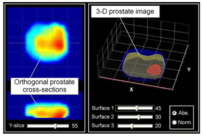
Representation of the prostate examination results. (Color version available online at http://ieeexplore.ieee.org.)
It enables physicians to literally see the differences in tissue stiffness on the color prostate images in contrast to DRE that is “blind” and relies exclusively on the clinician’s sense of touch. The PMI creates a hard copy of the prostate diagnostic procedure which can be placed into the patient’s file. This is advantageous for the physician on multiple fronts, as it gives the physician the ability to compare and contrast the patient’s results from year to year, and to get second opinions on the patient’s status in regards to the diagnosis.
III. Data Processing and Imaging Algorithms
Table I provides a list and a brief description of basic algorithms of PMI data processing and analysis incorporated in described imaging system. An expanded explanation of the algorithms is given below.
TABLE I.
Data Processing Algorithms
| Algorithm | Input | Procedures | Output | Purpose |
|---|---|---|---|---|
| Prostate image preprocessing and enhancement | Pressure sensor signal vs. time, raw pressure pattern | Temporal and 2-D spatial noise-removal filtering, signal threshold, prostate pixel extraction, convolution, pixel neighborhood rating based filtering, 2-D interpolation | 2-D prostate imprint | To improve the signal/noise ratio and to reveal certain features. To be used in image analysis, 2-D/3-D prostate image composition |
| Sphincter image formation | Raw pressure pattern in sphincter area | Temporal and spatial filtering, sphincter pixel identification, center mass calculation | 2-D dynamic sphincter image, sphincter coordinates | To be used in probe head positioning, sphincter visualization |
| Probe orientation calculation | Raw orientation sensor data | Signal filtering, tilt compensated magnetic sensor readings | Azimuth, elevation, rotation angles | To be used in probe head positioning, 2-D/3-D prostate image composition |
| 2-D matching and prostate image formation | 2-D prostate imprints, orientation data, sphincter coordinates | Matching calculation, image superposition, formation, and correction | 2-D composite prostate image | To be used in 3-D image formation, prostate feature extraction |
| 3-D prostate image composition | 2-D prostate imprints, 2-D composite prostate image | Image translation and superposition, 3-D interpolation and smoothing | 3-D prostate image | To be used in real time slice visualization, final 3-D pictorial visualization, feature calculations |
| Feature extraction | 2-D/3-D prostate images | Feature calculations | Calculated features | To be used in examination report, prostate evaluation |
| Examination data quality evaluation | Row pressure pattern sequence | Data are tested by criteria set | Data quality classification | Data characterization, to be used in training |
A. Prostate Image Preprocessing and Enhancement
Image enhancement techniques are used to improve an image, where “improving” is defined either objectively (e.g., increased signal-to-noise ratio), or subjectively (e.g., making certain features easier to see by modifying the colors or intensities). Fig. 5 illustrates image enhancement route using a real recorded raw pressure pattern over the prostate of a patient in the clinical study. The data from the pressure sensor arrays is preprocessed through the following procedures.
Fig. 5.
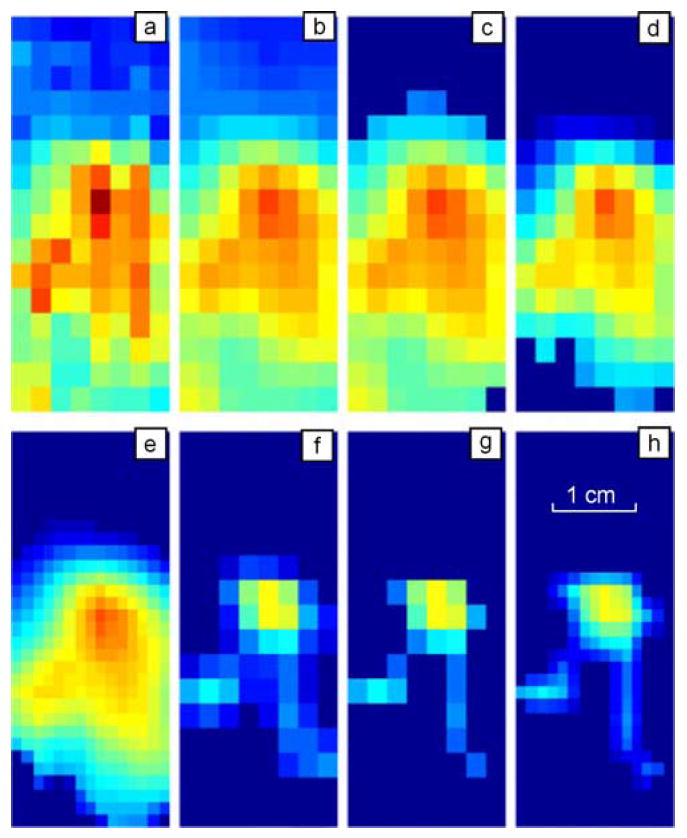
Illustration of the image processing sequence for pressure pattern recorded during single compression of the probe against the prostate in vivo. (a) Raw pressure pattern. (b) After temporal and spatial filters. (c) After threshold filter. (d) After prostate related signal extraction. (e) After interpolation. (f) After substructure segmentation to extract prostate inner features. (g) After pixel-wise filter. (h) After further interpolation. (Color version available online at http://ieeexplore.ieee.org.) (Color version available online at http://ieeexplore.ieee.org.)
Low-pass noise-cutting filtration based on the classical infinite impulse response Butterworth filter [39] of fourth order with cutoff frequency of 9 Hz was used as a primary procedure for preprocessing each pressure sensor signal.
Two-dimensional noise-removal filtration includes two steps. The first step is edge smoothing by linear filtration (weighed averaging of 3 × 2 pixels/sensors along the pressure sensor array boundary). The second step is a median filtering of 3 × 3 pixels/sensors inside the frame. Application of this filter after the low-pass filtering is illustrated in Fig. 5 where (a) and (b) show single raw and filtered 2-D pressure patterns, respectively.
Signal thresholding is widely used technique in image processing [40]. A parameter θ called the “brightness threshold” is chosen and applied to the image as follows: if brightness/intensity for a pixel is more than θ, this pixel value is not changed; if the brightness/intensity for a pixel is less than θ, this pixel value is changed to zero. We used the interactive technique developed by Ridler and Calvard for choosing the threshold [41]. The choice of the threshold is based on the histogram of the brightness scale that is initially segmented into two parts using a starting threshold value such as half the maximum dynamic range. The sample mean (mf,0) of the gray values is associated with the foreground pixels and the sample mean (mb,0) of the gray value is associated with the background pixels. A new threshold value θj is then computed as the average of these two sample means
| (1) |
The process is repeated, until the threshold value does not change any more, that is until θk = θk−1. The result of this procedure is shown in Fig. 5(c).
Prostate imprint extraction as a procedure for isolation of a partial prostate image consists of the separation of one or several relatively large coherent zones containing a relatively high pressure signal. Another purpose of this procedure is to reduce the influence of boundary effects and elimination of pressure peaks in the top and bottom parts of the probe head sensor array related to the sphincter and bladder pressure signals. This procedure starts with quadrupling the number of pixels in the image using two by two interpolations between neighboring sensors. The binary image of the pressure pattern is created by setting all pixels for which the pressure is higher than average to black. At the same time, the pixels for which the pressure is lower than average are set to white. Two types of filtering are applied thereafter to the binary image. The expanding filtering calculates the number of black pixels adjacent to each white point. If the number is higher than the predetermined value, it turns the white point into a black point in order to enlarge the black regions and cover small white holes. Then the second filtering is applied to achieve the same effect for black points. The number of white pixels adjacent to each black point is calculated and if that number is higher than the predetermined value, it turns that point to white, “squeezing” black zones and smoothing their edges. A sequence of these two types of filtering removes or significantly reduces small boundary defects, eliminates the inner white holes, combines and rounds large internal zones. The resulting black zone is mapped back to the pressure sensor array, and only the pressure sensors, which belong to the black zone, are allowed to participate in the next phase of the image analysis as shown in Fig. 5(d). Described procedure belongs to mathematical morphology which is often used as intuitive set of techniques useful for pattern recognition and spatial image filtering, taking measurements and knowledge out of image content, among others [42].
Following 2-D interpolation serves the purpose of image preparation for following processing and analysis. Matching procedure and prostate image formation are more effective if in the input we have an image of 31 × 15 pixels rather than 16 × 8. We used triangle-based cubic interpolation [43]. A prostate interpolated image is shown in Fig. 5(e).
Two-dimensional convolution filtering includes scanning across the image by a window of some finite size and shape. The output pixel value is the weighed sum of the input pixels within the window where the weights are the values of the filter assigned to every pixel of the window itself. The window with its weights is called the “convolution kernel,” denoted as h(j, k). Each new pixel c(m, n) will be equal to
| (2) |
where a(m, n) is the processed image, and J and K are the kernel window sizes. Fig. 5(f) shows the result of convolution filtering the image in Fig. 5(d). The simplest convolution kernel corresponding to a spherical nodule was applied.
Pixel neighborhood rating based filtering is a local point operation which calculates for each pixel having nonzero intensity its rating in the accordance with surrounding pixel intensities. If the pixel rating is less than some empirically predetermined value, this pixel value is changed to zero. This procedure helps more clearly extract the substructure inside the prostate as it may be seen in Fig. 5(g).
The result of the second 2-D interpolation applied to the image of Fig. 5(g) is shown in Fig. 5(h).
B. Sphincter Image Formation
Raw signals from the pressure sensor array mounted on the transrectal probe shaft for the sphincter imaging are processed using the same algorithms as are used for the analysis of the signals from the pressure sensor array located on the head of the probe, as described in Section II. A sphincter image is formed after temporal and spatial filtering of raw data and other steps described in Section III-A. Dynamic sphincter image formation has a time constant of about 3 s. The center of mass of the formed sphincter image is calculated, identifying thus the sphincter coordinates relative to the probe shaft. This information is further used for assessment of the prostate mobility.
C. Probe Orientation Calculation
The probe orientation tracking includes a three-axis magnetic sensor with orthogonal sensitivity axes Mx, My, Mz, and a two-axis acceleration sensor having sensitivity axes Ax, Ay, accordingly. Importantly, Ax-axis is parallel to the Mx-axis and Ay-axis is parallel to the My-axis. Both the magnetic sensor and the acceleration sensor are mounted on a platform inside the probe handle (see Fig. 1), so that X, Y plane is parallel to the probe head pressure sensing surface. Magnetic sensor readings give sensor orientation relative to the earth’s magnetic field. To compensate the magnetic sensor reading for X, Y —platform tilt relative to a horizontal plane, which is perpendicular to earth’s gravity vector, it is necessary to know the platform tilt angles. The 2-D accelerometer sensor is used as a tilt sensor to provide elevation (φ) and rotation (θ) readings. The X, Y, Z magnetic readings can be traced back to the horizontal plane by applying the rotational equations [36]
| (3) |
| (4) |
where X h and Y h are earth’s magnetic vector projections to the horizontal plane. Once X h and Y h are known, we can calculate an azimuth angle Az as
| (5) |
The azimuth angle A z is used as a key parameter in probe positioning relative to the prostate during 2-D prostate image formation (see next Section). Knowing current A z and distance between the sphincter and the center of the probe head pressure sensing surface one can calculate the transverse (Y coordinate) and longitudinal (X coordinate) probe head location relative to the start one defined in the moment of pressing start/reset button on the probe handle.
D. Two-Dimensional Matching and Prostate Image Formation
An important advantage of the use of 2-D pressure sensor array is possibility to use the prostate itself as a reference point. After acquisition of prostate imprints from the first 2-D processed prostate patterns, 2-D prostate image formation is accomplished in the next few steps by the means of constructing the composite prostate image. Specifically, after pressing the start/reset button on the probe handle the first n frames of pressure response data are captured to construct a starting fragment of the prostate image. This capture occurs when the total pressure prostate signal exceeds a predetermined threshold. After averaging, the captured starting fragment of the prostate image is transferred into a 2-D composite prostate image. Then each subsequent prostate pressure response data frame is recorded and analyzed in order to place new pressure response information into the 2-D composite prostate image. A separate operational module runs a matching algorithm, which tries to find the best fit for the every prostate imprint within the 2-D composite prostate image inside the spatial limits imposed by the probe head sensors position calculated from the orientation data and sphincter coordinates. Preferably, the best fit is calculated by maximizing a functional F
| (6) |
where k and l are quantities of horizontal and vertical pixels inside the pressure frame with the current pressure response pattern of the prostate, n and m are image shift in pixels relative to a previous fitted pattern, Si, j is current pressure response signal of i, j pixels, and Pn+i,m+j is a pressure signal of n + i, m + j, pixel inside the 2-D composite prostate image. The probe position calculated according to the procedure of Section III-C imposes limitations on n and m ranges for finding the best image fit. Such simple matching calculation procedure has been chosen for the reason of the limited computer power in real-time analysis mode.
After the best fit is found, each pixel of the prostate imprint is placed into the 2-D composite prostate image with a predetermined weighted factor if its current value exceeds respective pixel value inside the 2-D composite prostate image. All calculations are implemented with normalized pixels, so that each pixel value of the prostate imprint is divided by a modified average of analyzed pressure pattern. The modified average S̄ is calculated according to (7) after removing a predetermined quantity (b) of pressure pixels Smax having maximum values
| (7) |
where k and l are quantities of horizontal and vertical pixels inside the pressure response frame with the analyzed prostate pattern, Si, j is the current pressure signal of i, j pixels.
E. Three-Dimensional Prostate Image Reconstruction
The 3-D prostate image includes a plurality of 2-D prostate imprints placed inside planes ranged against the total pressure applied to prostate by the probe head pressure sensors. Each 2-D prostate imprint is processed according to algorithms described in Sections III-A and III-B, and is then translated inside the 3-D prostate image where X, Y coordinates are determined by matching algorithm described in Section III-D, and Z coordinate is proportional to S̄ calculated according to (7). Each pixel of the translated 2-D prostate imprint is then placed inside the 3-D prostate image with a predetermined weighted factor if its current pixel value exceeds a threshold value inside the 3-D prostate image. Two different 3-D prostate images are constructed: one image includes only normalized pressure response pixels (each pixel value of the prostate image is divided by a modified average of analyzed pressure response data frame), while another image includes only absolute pressure response pixels. This helps to separate prostate form factor signals from nodule signal. After prostate examination is complete, a final smoothing and 3-D interpolation is applied to the constructed structures. The final 3-D data arrays are then used to prepare slices, iso-surfaces and alike for structure visualization.
F. Prostate Feature Calculation
Geometrical characteristics of the prostate, such as prostate size and shape are calculated directly from the final prostate images. A nodule detection algorithm includes four separate nodule detectors having in input both 2-D prostate pressure pattern sequence and 3-D prostate image. Prostate consistency/hardness is evaluated from a prostate image gradient analysis for increasing prostate signals. Prostate mobility is estimated as prostate ability to change position relative to the sphincter as a result of probe pressing against the prostate.
Prostate size is calculated in terms of both a cross section area A and the prostate longitudinal dimension L in the frontal (coronal) plane using 3-D prostate image composed from the absolute pressure response pixels P, as described in Section III-E. This 3-D prostate image may be represented as P(x, y, Z), where Z coordinate is considered proportional to S̄ calculated by means of the expression (7). Thus, A may be written as
| (8) |
where Pb(x, y, Z, Th) is binary transformation of P(x, y, Z); Th is a threshold pressure level which corresponds to the physical prostate boundary
| (9) |
A(Th, Z), as a function of Z, reaches a stationary value which is accepted as the prostate cross section area. To evaluate L, another procedure calculates from the Pb(x, y, Z, Th) linear sizes along Y coordinate for the prostate center, left and right prostate lobes. Wherein each linear size, e.g., for the prostate center Lpc, is calculated as
| (10) |
Here, q is an empirically predetermined range of Z value, xpc is the transverse coordinate of the prostate center. Then, the prostate longitudinal size L is calculated as an average of these three linear sizes.
Prostate shape features, such as symmetry and median groove, are calculated directly from the 3-D binary prostate image denoted as Pb(x, y, Z, Th). The prostate symmetry may be characterized by the ratio of left (Vl)/right (Vr) prostate lobe volumes calculated as
| (11) |
| (12) |
To characterize the prostate median groove, which looks like a gully between the left and right prostate lobes, we calculate median groove relative depth D according to the following procedure. At first, we calculate P(x, Th) as a function of prostate cross section area along transverse X coordinate
| (13) |
If this function has saddle-shaped appearance, then we say that median groove is present and D is calculated as
| (14) |
where l index denotes local maximum corresponding to the left prostate lobe, r index corresponds to the right local maximum, and c index corresponds to the local minimum of the P(x, Th) function between the prostate lobes.
Prostate nodule detection is formalized by calculation of two values: nodule size and nodule strength. The nodule size Na is calculated as cross section area above predetermined threshold ThN in the 3-D prostate normalized image Pn(x, y, Z) as
| (15) |
| (16) |
The nodule strength Ns is calculated as the maximum inside Pn(x, y, Z) according to
| (17) |
| (18) |
Condition (18) is a constrain for possible x, y, Z coordinates inside the 3-D prostate image where Ns is calculated, h is a predetermined thickness of the prostate surface layer. Physical meaning of this constrain is to exclude pixels close to the prostate surface and remove possible high level signals caused by the curvature of prostate lobes from 3-D prostate normalized image. If both calculated values extend beyond the 2-D prostate normal bounds in Na – Ns metrics, nodule detection classifier is signaling the presence of a nodule.
Prostate hardness Pc was calculated as an averaged pressure over an area limited by closed iso-line corresponding to an empirically chosen level ph in 2-D prostate imprint under the condition that this prostate imprint area is inside a predetermined area Pa ± Δ and the probe head is moving towards to the prostate. Formal expression used for calculation of prostate hardness Pc is
| (19) |
| (20) |
| (21) |
| (22) |
where Pυn is an average prostate imprint value calculated according to (21); N is a number of frames satisfying condition (20); Pa = 2.0 cm2 is the fixed area, k and l are quantities of horizontal and vertical pixels inside pressure response frame, Si, j is the current pressure signal of i, j pixels; ph = 15 kPa is the threshold value.
Prostate mobility is defined as a range of prostate displacement during examination evaluated from the data on changes in the prostate position relative to the sphincter.
G. Examination Data Quality Evaluation
This algorithm detects the prostate pressure imprint in each pressure pattern recorded from the probe head pressure sensor array. It estimates the probability that the prostate is under the sensor array. The possibility that some sensors could produce an erroneous signal, as well as that some rows and column in the sensor array could have incorrect tuning or calibrating are taken into account. Such column and row errors may cause false pressure jumps or gaps in the pressure pattern. For each interior row or column of the sensor array, the detection algorithm calculates a pressure signal value relative to the linear interpolation based on the boundary pressure. A predetermined number of points with highest and lowest pressure values are discarded. The positive or negative sign of the sum of remaining values defines the sign of the entire line. Each line (row or column) is assigned a certain weight, the highest for the central lines, and the lowest for boundary lines. If the sum of the weights for all lines with corresponding signs is greater than a predefined value, it is considered that the mechanical image contains the prostate imprint. The sum is then normalized to a predetermined range, using two scale parameters estimating the presence of a prostate imprint in the image. Total quantity of data frames including prostate related signal with at least 50% probability is calculated. The pressure sensor average range, probe orientation range, and number of pressings against the prostate are calculated as well. Then a simple, additive, linear classifier ascribes the data quality level to collected prostate examination data: A (good), B (problematic), or C (poor). This way, the operator has feedback which characterizes the quality and confidence level of the examination outcome.
IV. Results of Laboratory and Clinical Studies
A. Prostate Phantom Experiments
Laboratory testing on the prostate phantoms demonstrated that just five successive pressings of the probe against the phantom are sufficient to provide clear integrated image, such as that shown in Fig. 6. Upper row of images in Fig. 6 shows five 2-D patterns used for creating the integrated mechanical image of the phantom. Lower panels in Fig. 6 show a comparison of the integrated image (left) with the picture of the examined phantom (right). Fig. 7 illustrates the reproducibility of the PMI examination data. The examined prostate phantom had elasticity modulus 33 kPa (±3 kPa) and a hard round inclusion with 9 mm diameter molded in left lobe. The phantom was examined repeatedly nine times by the same operator. Composed 2-D orthogonal cross sections of the phantom are represented in Fig. 7. Table II presents a comparison of the phantom parameters evaluated by PMI with the actual values obtained by direct geometrical and elasticity measurements [32], [44].
Fig. 6.
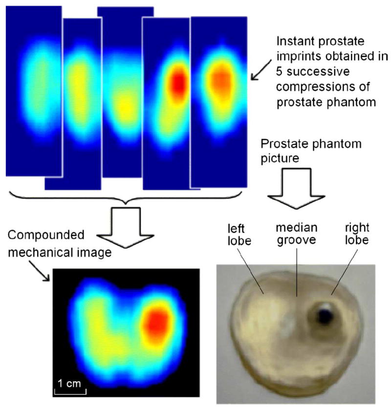
Imaging of a prostate phantom with a hard nodule. Image is obtained by compounding five successive pressure patterns. (Color version available online at http://ieeexplore.ieee.org.)
Fig. 7.
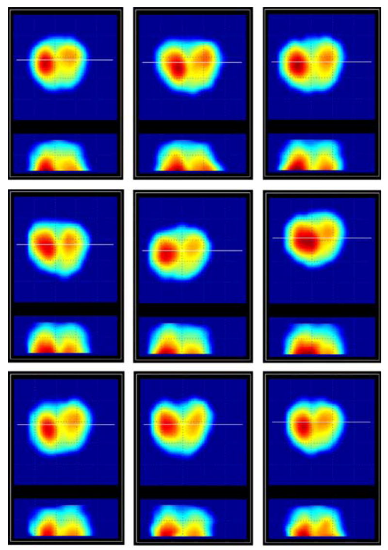
Repeat scans of the same prostate phantom. (Color version available online at http://ieeexplore.ieee.org.)
TABLE II.
PMI Performance for Nine Scans of the Same Phantom (Center Column) Against the Directly Measured Phantom Parameters (Right Column)
| Prostate feature | Calculated parameters (average ± STD) | Measured parameters (average ± STD) |
|---|---|---|
| Symmetry (ratio of left/right areas) | 0.88 ± 0.06 | 0.92 ± 0.05 |
| Median groove (relative depth) | 0.23 ± 0.08 | 0.15 ± 0.05 |
| Longitudinal size, mm | 23 ± 1 | 23 ± 1 |
| Nodule presence | Yes | Yes |
| Nodule size, cm2 | 0.75 ± 0.06 | 0.81 ± 0.02 |
| Nodule strength, rel. units | 74 ± 2 | n/a |
| Integral hardness, kPa | 38 ± 5 | 33 ± 6 |
| Mobility (displacement range), mm | 8.9 ± 1.9 | 7.0 ± 3.0 |
B. Clinical Results
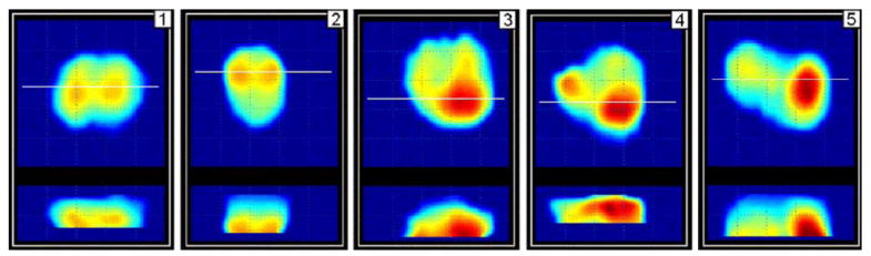
Table III and Fig. 8 present results of the study conducted at the Robert Wood Johnson University Hospital, New Brunswick, NJ, on five patients aged between 58 and 81. Eligible participants were informed about the nature of the investigation and signed an informed consent form. Upon patient’s consent, relevant clinical and demographical data were recorded (history of prostate disease and corresponding treatment, family history of prostate cancer, race, and age), and all participants completed the American Urological Association (AUA) symptom index questionnaire.
TABLE III.
Clinical Data for Five Patients
| Prostate feature | Patient’s number | ||||
|---|---|---|---|---|---|
| 1 | 2 | 3 | 4 | 5 | |
| Symmetry (ratio of left/right areas) | 0.95 | 0.94 | 0.87 | 0.73 | 0.88 |
| Median groove (relative depth) | 0.20 | 0.03 | 0.32 | 0.22 | 0.32 |
| Longitudinal size, mm | 25 | 28 | 29 | 27 | 25 |
| Nodule presence | No | No | Yes | Yes | Yes |
| Nodule size, cm2 | (0.03) | (0.17) | 0.64 | 0.93 | 1.0 |
| Nodule strength, rel. units | (41) | (45) | 60 | 66 | 81 |
| Integral hardness, kPa | 23 | 17 | 31 | 23 | 43 |
| Mobility (displacement range), mm | 7 | 16 | 5 | 9 | 11 |
Fig. 8.
Orthogonal cross sections of prostate of five patients examined by PMI at the Robert Wood Johnson University Hospital. (Color version available online at http://ieeexplore.ieee.org.)
PMI compounded 2-D orthogonal cross section images of the examined prostates are represented in Fig. 8; the calculated prostate features are given in Table III. The threshold values used in clinical data processing were the same as used in laboratory phantom testing. Horizontal white line in each upper X, Y image corresponds to the location of X, Z cross section, which are in lower part of the panel of Fig. 8.
V. Discussion
Two-dimensional and 3-D prostate image formation algorithms, described in Section III-D and III-E, take as the input a sequence of 2-D prostate imprints extracted from the raw pressure patterns recorded by the pressure sensor array mounted on the head of transrectal probe (see Fig. 1). Low-pass noise-cutting Butterworth filter applied to primary sensor signal seemed to be more effective than Chebyshev Types I and II, elliptic, Bessel, and other filter types [45]. The main advantage of infinite impulse response filters over finite impulse response (FIR) filters is that they typically meet a given set of specifications with a much lower filter order than a corresponding FIR filter and allow time efficient C++ implementation [46]. The median filtering is similar to an averaging filter, in which each output pixel is set to an “average” of the values. However, with median filtering, the value of an output pixel is determined by the median of the neighboring pixels, rather than the mean. The median filter is less sensitive to extreme values (the outliers) than the mean and, therefore, can better remove these outliers without reducing the sharpness of the image [47]. Two-dimensional convolution filtering is not just pragmatic procedure for smoothing or sharpening an image. This procedure allows amplifying structures similar to the used convolution kernel. That is if we know certain characteristic structural features of possible lesions, we can apply a set of prepared convolution kernels, one after another, to determine what kind of kernel better reveals the underlying structure [43].
A pressure response pattern may be expressed as S(x, y), where x, y are sensor coordinates in the pressure sensor array of the probe head. Every pattern including the prostate in absolute or in normalized form is placed according to the specified location into 2-D and 3-D prostate images. In 3-D prostate image formation, for example, S(x, y) is placed by a parallel translation inside the prostate image P(x, y, Z). Z-coordinate is calculated according to expression (7). This is a rough approximation for the inverse problem solution [48] and it is surprising, that even this very simple approach could provide practical results. Z scale may become geometrically erroneous in the event that prostate tissues stiffen under the applied load [28], [49], but at any case Z scale reflects the depth dependence. Better results were obtained by extracting substructures Si(x, y) inside prostate imprint (see panel 8 in Fig. 5) and keeping track of these substructures separately from the whole prostate. From these observations, we see great reserve for the MI in development and exploration a deformable prostate model.
Table II summarizes the average calculated prostate phantom features and the standard deviation (STD) for nine repeat scans performed by the same person. Automatically composed cross sectional images for these nine examinations are represented in Fig. 7. This experiment reveals reproducibility for feature calculations. We can observe in Fig. 7 variability in the 2-D compound image of the phantom due to deformation of the phantom during pressing against its surface by the probe head. Current prostate image composition algorithms, as we mentioned, do not include any deformable model to capture a variety of possible deformations and to convert them to an invariant structure. The quantitative characteristic of this variability for calculated longitudinal prostate size is ranged inside 5%. The prostate cross section area calculated according to expression (8) has STD of 6%. The symmetry and the median groove detection ratios have STD within 9%. Nodule size detector has STD about 8% and nodule strength STD is less than 3%. Standard deviation of about 13% for the integral hardness calculations may be accepted as satisfactory for used simple procedure according to (19)-(22). Direct phantom hardness measurements hardly may provide accuracy better than 20%. Two-millimeter accuracy in the prostate mobility evaluation by PMI can be considered acceptable too. Thus, PMI examination, guided by real-time prostate and sphincter images, allows obtaining compound mechanical images of prostate phantom and quantitative evaluation of its size, shape, hardness, nodularity, and mobility.
In all five clinical cases described in Section IV-B, PMI has automatically calculated the prostate features and represented the compounded prostate images (see Table III and Fig. 8). These results demonstrate both the advantages and limitations of the technology. The range of prostate longitudinal linear sizes evaluated by PMI, as shown in Fig. 8, are in close agreement with prostate sizes evaluated by transrectal ultrasound [50]. Such prostate features as prostate symmetry and median groove can be assessed by an operator not only from the calculated numeric values, but by visual analysis of orthogonal prostate cross sections. According to the recorded clinical history of the prostate disease for the patients 3–5, their prostates might be having nodularity, while the patients 1 and 2 has no signs of the prostate abnormality. These facts are in a good agreement with PMI findings as seen from Table III. We may observe also that the integral prostate hardness has an upward bias with the detected nodularity. Yet, we can not make conclusion about possible interrelation of prostate mobility and nodularity from the received data. In general, this clinical testing clearly demonstrates that PMI has the ability to reconstruct the prostate mechanical image and quantitatively evaluate its diagnostically relevant features.
PMI has potential to become a diagnostic tool that could replace DRE. Theoretically and practically, MI sensitivity is higher than a human finger [30]-[33], which may detect prostate cancer only having volume about 0.2 mL or larger [51]. Another factor that dilutes the usefulness of DRE is its limited reproducibility. In a relatively small study including 116 volunteers, the kappa of agreement among eight urologists, fellows, and residents was 0.22 [52]. As regarding the prostate size evaluation, estimates with DRE of prostate weight by multiple examiners in a large prostate cancer screening study (more 36 000 men) correlated poorly with radical retropubic prostatectomy specimen weight (r = 0.27) [53].
Another potential niche and clinical benefits of the use of MI technology could be in expectant management (also referred to as deferred treatment) which involves actively monitoring the course of the disease with the expectation to intervene if the cancer progresses or if symptoms become imminent [54]. Watchful waiting being included into the expectant management refers to no treatment [55], [56]. Patients on expectant management are likely to have progression of their tumors but with different rate. Unfortunately, the currently established prognostic factors cannot accurately tell which patients will have a slow or a rapid prostate cancer progression [57]. For patients with a life expectancy of 10 years or more and who therefore might benefit from definitive local therapy, monitoring including PSA determination and DRE every six months is recommended [57]. PMI may provide here the documented history of the expectant management.
DRE is also performed to assess whether or not there is any sign of local disease recurrence after treatment with curative intent [58]. It is very difficult to interpret the findings of DRE after curative therapy, especially after radiotherapy. A newly detected nodule should raise the suspicion of local disease recurrence. A local disease recurrence after curative treatment is possible without a concomitant rise in PSA level [59]. Thus, PMI could be useful here too because for asymptomatic patients, a disease-specific history and PSA measurement supplemented by DRE are the recommended tests for routine follow-up. These should be performed at three, six, and 12 months after treatment, then every six months until three years, and then annually [60]. How can an urologist remember his impression that has been acquired by DRE three or six months ago when tens patients a day may go through his attention? The use of PMI in everyday practice will provide hardcopy with 2-D/3-D prostate images accompanied by the calculated prostate features.
VI. Conclusion
MI technology provides documented 3-D mechanical prostate image with quantitative evaluation of prostate features such as size, shape, hardness, nodularity, and mobility, which is much superior to the outcome of DRE, one of the current means for prostate cancer screening. MI has a potential to be positioned as an objective substitute for DRE in screening for prostate cancer, in expectant management, and in an assessment whether or not there is any sign of local disease recurrence after treatment with curative intent that can potentially improve an early-stage diagnosis and treatment of prostate cancer.
Acknowledgments
The authors would like to acknowledge the assistance of the R. E. Weiss of the Division of Urology, Robert Wood Johnson Medical School in clinical study. Thy would also like to thank S. Kanilo of Artann Laboratories for development and implementation of a core data acquisition and data management engine for PMI.
This work was supported in part by the National Institute of Health (NIH) under SBIR Grant 2 R44 CA82620-02 entitled “Portable mechanical imaging device for prostate cancer detection.
References
- 1.Jemal A, Murray T, et al. Cancer statistics, 2005. CA Cancer J Clin. 2005;55:10–30. doi: 10.3322/canjclin.55.1.10. [DOI] [PubMed] [Google Scholar]
- 2.Brawer MK, Chetner MP. Ultrasonography of the prostate and biopsy. In: Walsh PC, Retik AB, Vaughan ED Jr, Wein AJ, editors. Campbell’s Urology. 7. 82. Philadelphia, PA: Saunders; 1998. pp. 2506–2517. [Google Scholar]
- 3.Harris RP, Lohr KN, Beck R, Fink K, Godley P, Bunton A. Screening for prostate cancer systematic evidence review no. 16. Rockville, MD: Agency for Healthcare Research and Quality; Dec, 2001. [PubMed] [Google Scholar]
- 4.Mistry K, Cable G. Meta-analysis of prostate-specific antigen and digital rectal examination as screening tests for prostate carcinoma. J Amer Board Family Pract. 2003;16:95–101. doi: 10.3122/jabfm.16.2.95. [DOI] [PubMed] [Google Scholar]
- 5.Mettlin C, Murphy GP, et al. The results of a five-year early prostate cancer detection intervention. Cancer. 1996;77:150–159. doi: 10.1002/(SICI)1097-0142(19960101)77:1<150::AID-CNCR25>3.0.CO;2-3. [DOI] [PubMed] [Google Scholar]
- 6.Catalona WJ, Richie JP, et al. Comparison of digital rectal examination and serum prostate specific antigen in the early detection of prostate cancer: Results of a multicenter clinical trial of 6,630 men. J Urol. 1994;151:1283–1290. doi: 10.1016/s0022-5347(17)35233-3. [DOI] [PubMed] [Google Scholar]
- 7.Sarvazyan AP. Mechanical imaging: A new technology for medical diagnostics. Int J Med Inf. 1998;49:195–216. doi: 10.1016/s1386-5056(98)00040-9. [DOI] [PubMed] [Google Scholar]
- 8.Ophir J, Cespedes I, Ponnekanti H, Yazdi Y, Li X. Elastography: A quantitative method for imaging the elasticity of biological tissues. Ultrason Imag. 1991;13:11–134. doi: 10.1177/016173469101300201. [DOI] [PubMed] [Google Scholar]
- 9.Skovoroda AR, Emelianov SY, Lubinski MA, Sarvazyan AP, Odonnell M. Theoretical-analysis and verification of ultrasound displacement and strain imaging. IEEE Trans Ultrason Ferroelect Freq Control. 1994 May;41(3):302–313. [Google Scholar]
- 10.Sarvazyan AP, Skovoroda AR, et al. Biophysical bases of elasticity imaging. In: Jones JP, editor. Acoustical Imaging. Vol. 21. New York: Plenum; 1995. pp. 223–240. [Google Scholar]
- 11.Muthupillai R, Lomas DJ, et al. Magnetic-resonance elastography by direct visualization of propagating acoustic strain waves. Science. 1995;269:1854–1857. doi: 10.1126/science.7569924. [DOI] [PubMed] [Google Scholar]
- 12.Sarvazyan AP, Rudenko OV, Swanson SD, Fowlkes JB. Shear wave elasticity imaging: A new ultrasonic technology of medical diagnostics. Ultrasound Med Biol. 1998;24(9):1419–1435. doi: 10.1016/s0301-5629(98)00110-0. [DOI] [PubMed] [Google Scholar]
- 13.Plewes DB, Bishop J, Samani A, Sciarretta J. Visualization and quantification of breast cancer biomechanical properties with magnetic resonance elastography. Phys Med Biol. 2000;45:1591–1610. doi: 10.1088/0031-9155/45/6/314. [DOI] [PubMed] [Google Scholar]
- 14.Taylor LS, Porter BC, Rubens DJ, Parker KJ. Three-dimensional sonoelastography: Principles and practices. Phys Med Biol. 2000;45:1477–1494. doi: 10.1088/0031-9155/45/6/306. [DOI] [PubMed] [Google Scholar]
- 15.Manduca A, Oliphant TE, et al. Magnetic resonance elastography: Non-invasive mapping of tissue elasticity. Med Image Anal. 2001;5:237–254. doi: 10.1016/s1361-8415(00)00039-6. [DOI] [PubMed] [Google Scholar]
- 16.Nightingale K, Soo MS, Nightingale R, Trahey G. Acoustic radiation force impulse imaging: In vivo demonstration of clinical feasibility. Ultrasound Med Biol. 2002;28(2):227–235. doi: 10.1016/s0301-5629(01)00499-9. [DOI] [PubMed] [Google Scholar]
- 17.Greenleaf JF, Fatemi M, Insana M. Selected methods for imaging elastic properties of biological tissues. Annu Rev Biomed Eng. 2003;5:57–78. doi: 10.1146/annurev.bioeng.5.040202.121623. [DOI] [PubMed] [Google Scholar]
- 18.Washington CW, Miga MI. Modality Independent Elastography (MIE): A new approach to elasticity imaging. IEEE Trans Med Imag. 2004 Sep;23(9):1117–1128. doi: 10.1109/TMI.2004.830532. [DOI] [PubMed] [Google Scholar]
- 19.McCracken PJ, Manduca A, Felmlee J, Ehman RL. Mechanical transient-based magnetic resonance elastography. Magn Reson Med. 2005;53:628–639. doi: 10.1002/mrm.20388. [DOI] [PubMed] [Google Scholar]
- 20.Rubens DJ, Hadley MA, et al. Sonoelasticity imaging of prostate cancer: in vitro results. Radiology. 1995;195(2):379–383. doi: 10.1148/radiology.195.2.7724755. [DOI] [PubMed] [Google Scholar]
- 21.Dresner MA, Rose GH, Rossman PJ, Muthupillai R, Ehman RL. Magnetic resonance elastography of the prostate. Radiology. 1998;209P:152. doi: 10.1002/1522-2586(200102)13:2<269::aid-jmri1039>3.0.co;2-1. [DOI] [PubMed] [Google Scholar]
- 22.Lorenz A, Ermert H, et al. Ultrasound elastography of the prostate. A new technique for tumor detection. Ultraschall Med. 2000;21(1):8–15. doi: 10.1055/s-2000-8926. in German. [DOI] [PubMed] [Google Scholar]
- 23.Cochlin DL, Ganatra RH, Griffiths DF. Elastography in the detection of prostatic cancer. Clin Radiol. 2002;57(11):1014–1020. doi: 10.1053/crad.2002.0989. [DOI] [PubMed] [Google Scholar]
- 24.Souchon R, Rouviere O, et al. Visualisation of HIFU lesions using elastography of the human prostate in vivo: Preliminary results. Ultrasound Med Biol. 2003;29(7):1007–1015. doi: 10.1016/s0301-5629(03)00065-6. [DOI] [PubMed] [Google Scholar]
- 25.Kemper J, Sinkus R, Lorenzen J, Nolte-Ernsting CC, Adam G. MR elastography of the prostate: Initial in-vivo application. Fortsch Röntgenstr. 2004;176(8):1094–1099. doi: 10.1055/s-2004-813279. in German. [DOI] [PubMed] [Google Scholar]
- 26.Konig K, Scheipers U, et al. Initial experiences with real-time elastography guided biopsies of the prostate. J Urol. 2005;174:115–117. doi: 10.1097/01.ju.0000162043.72294.4a. [DOI] [PubMed] [Google Scholar]
- 27.Curiel L, Souchon R, Rouviere O, Gelet A, Chapelon JY. Elastography for the follow-up of high-intensity focused ultrasound prostate cancer treatment: Initial comparison with MRI. Ultrasound Med Biol. 2005 Nov;31(11):1461–1468. doi: 10.1016/j.ultrasmedbio.2005.06.013. [DOI] [PubMed] [Google Scholar]
- 28.Krouskop TA, Wheeler TM, Kallel F, Garra BS, Hall T. Elastic moduli of breast and prostate tissues under compression. Ultrason Imag. 1998;20(4):260–274. doi: 10.1177/016173469802000403. [DOI] [PubMed] [Google Scholar]
- 29.Sarvazyan AP. Elastic properties of soft tissues. In: Levy M, Bass HE, Stern RR, editors. Handbook of Elastic Properties of Solids, Liquids and Gases. 5. III. New York: Academic; 2001. pp. 107–127. [Google Scholar]
- 30.Sarvazyan AP. Computerized palpation is more sensitive than human finger. Proc 12th Int Symp Biomed Meas Instrum; Dubrovnik, Croatia. 1998. pp. 523–524. [Google Scholar]
- 31.Niemczyk P, Sarvazyan AP, et al. Mechanical imaging, A new technology for cancer detection. Surgical Forum. 1996;47:823–825. [Google Scholar]
- 32.Niemczyk P, Cummings KB, Sarvazyan AP, Bancila E, Ward WS, Weiss RE. Corelation of mechanical imaging and histopathology of radical prostatectomy specimens: A pilot study for detecting prostate cancer. J Urol. 1998;160:797–801. doi: 10.1016/S0022-5347(01)62790-3. [DOI] [PubMed] [Google Scholar]
- 33.Weiss RE, et al. In vitro trial of the pilot prototype of the prostate mechanical imaging system. Urology. 2001;58(6):1059–1063. doi: 10.1016/s0090-4295(01)01407-8. [DOI] [PubMed] [Google Scholar]
- 34.Freeman HJ. Documentation of rectal examination performance in the clinical teaching unit of a university hospital. Can J Gastroenterol. 2000;14:272–276. doi: 10.1155/2000/297390. [DOI] [PubMed] [Google Scholar]
- 35.Turner KJ, Brewster SF. Rectal examination and urethral catheterization by medical students and house officers: Taught but not used. Br J Urol Int. 2000;86:422–426. doi: 10.1046/j.1464-410x.2000.00859.x. [DOI] [PubMed] [Google Scholar]
- 36.Howe RD, Peine WJ, Kontarinis DA, Son JS. Remote palpation technology. IEEE Eng Med Biol Mag. 1995 May/Jun;14(3):318–323. [Google Scholar]
- 37.Caruso MJ. Application of magnetoresistive sensors in navigation systems Honeywell SSEC, 2005 [Online] Available: http://www.ssec.honeywell.com/magnetic/datasheets/sae.pdf.
- 38.Pujol S, Pecher M, Magne JL, Cinquin P. A virtual reality based navigation system for endovascular surgery. Stud Health Technol Inf. 2004;98:310–312. [PubMed] [Google Scholar]
- 39.Selesnick IW, Burrus CS. Generalized digital butterworth filter design. IEEE Trans Signal Process. 1998 Jun;46(6):1688–1694. [Google Scholar]
- 40.Gonzalez RC, Woods RE. Digital Image Processing. New York: Addison-Wesley; 2002. [Google Scholar]
- 41.Ridler TW, Calvard S. Picture thresholding using an iteractive seletion method. IEEE Trans Syst Man Cybern. 1978 Aug;SMC-8(8):630–632. [Google Scholar]
- 42.Soille P. Morphological Image Analysis. 2. New York: Springer; 2004. [Google Scholar]
- 43.Louis AK, Schuster TA. Novel filter design technique in 2D computerized tomography. Inverse Problems. 1996;12:685–696. [Google Scholar]
- 44.Sarvazyan T, Stolarsky V, Fishman V, Sarvazyan AP. Development of mechanical models of breast and prostate with palpable nodules. Proc 20th Annu Int Conf IEEE Eng Med Biol Soc; 1998. pp. 736–739. [Google Scholar]
- 45.Antoniou A. Digital Filters: Analysis, Design, and Applications. 2. New York: McGraw-Hill; 1993. [Google Scholar]
- 46.Mitra SK. Digital Signal Processing: A Computer-Based Approach. New York: McGraw-Hill; 1998. [Google Scholar]
- 47.Young TI, Gerbrands JJ, van Vliet LJ. Fundamentals of Image Processing. Delft, The Netherlands: Delft Univ Technol; 1998. [Google Scholar]
- 48.Oberai1 AA, Gokhale1 NH, Feijóo GR. Solution of inverse problems in elasticity imaging using the adjoint method. Inverse Problems. 2003;19:297–313. [Google Scholar]
- 49.Erkamp RQ, Emelianov SY, Skovoroda AR, Chen X, O’Donnell M. Exploiting strain-hardening of tissue to increase contrastin elasticity imaging. Proc IEEE Ultrason Symp. 2000;2:1833–1836. [Google Scholar]
- 50.Sech S, Montoya J, Girman CJ, Rhodes T, Roehrborn CG. Interexaminer reliability of transrectal ultrasound for estimating prostate volume. J Urol. 2001;166:125–129. [PubMed] [Google Scholar]
- 51.Smith JA, Jr, Scardino PT, Resnick MI, Hernandez AD, Rose SC, Egger MJ. Transrectal ultrasound versus digital rectal examination for the staging of carcinoma of the prostate: Results of a prospective multi-institutional trial. J Urol. 1997;157:902–906. [PubMed] [Google Scholar]
- 52.Smith DS, Catalona WJ. Interexaminer variability of digital rectal examination in detecting prostate cancer. Urology. 1995;45:70–74. doi: 10.1016/s0090-4295(95)96812-1. [DOI] [PubMed] [Google Scholar]
- 53.Loeb S, et al. Accuracy of prostate weight estimation by digital rectal examination versus transrectal ultrasonography. J Urol. 2005;173:63–65. doi: 10.1097/01.ju.0000145883.01068.5f. [DOI] [PubMed] [Google Scholar]
- 54.Patel MI, Concini DT, et al. An analysis of men with clinically localized prostate cancer who deferred definitive therapy. J Urol. 2004;171:1520–1524. doi: 10.1097/01.ju.0000118224.54949.78. [DOI] [PubMed] [Google Scholar]
- 55.Johansson JE, Andren O, et al. Natural history of early, localized prostate cancer. J Amer Med Assoc. 2004;291:2713–2719. doi: 10.1001/jama.291.22.2713. [DOI] [PubMed] [Google Scholar]
- 56.Bill-Axelson A, Holmberg L, et al. Radical prostatectomy versus watchful waiting in early prostate cancer. New Eng J Med. 2005;352:1977–1984. doi: 10.1056/NEJMoa043739. [DOI] [PubMed] [Google Scholar]
- 57.NCCN. Clinical practice guidelines in oncology. Prostate Cancer. 2005;2:1–44. [Google Scholar]
- 58.Harris R, et al. Screening for prostate cancer. Systematic evidence review Agency for Healthcare Research and Quality U.S. Department of Health and Human Services, 16, Oct. 2002 [Online] Available: http://www.ahrq.gov.
- 59.Oefelein MG, Smith N, Carter M, Dalton D, Schaeffer A. The incidence of prostate cancer progression with undetectable serum prostate specific antigen in a series of 394 radical prostatectomies. J Urol. 1995;154:2128–2131. [PubMed] [Google Scholar]
- 60.Aus G, et al. Guidelines on prostate cancer European Association of Urology, Feb. 2003 [Online] Available: http://www.uroweb.org/files/uploaded_files/guidelines/prostate_cancer.pdf.