IMRT treatment planning for prostate cancer using prioritized prescription optimization and mean-tail-dose functions

Abstract

Treatment planning for intensity modulated radiation therapy (IMRT) is challenging due to both the size of the computational problems (thousands of variables and constraints) and the multi-objective, imprecise nature of the goals. We apply hierarchical programming to IMRT treatment planning. In this formulation, treatment planning goals/objectives are ordered in an absolute hierarchy, and the problem is solved from the top-down such that more important goals are optimized in turn. After each objective is optimized, that objective function is converted into a constraint when optimizing lower-priority objectives. We also demonstrate the usefulness of a linear/quadratic formulation, including the use of mean-tail-dose (mean dose to the hottest fraction of a given structure), to facilitate computational efficiency. In contrast to the conventional use of dose-volume constraints (no more than x% volume of a structure should receive more than y dose), the mean-tail-dose formulation ensures convex feasibility spaces and convex objective functions. To widen the search space without seriously degrading higher priority goals, we allowed higher priority constraints to relax or ‘slip’ a clinically negligible amount during lower priority iterations. This method was developed and tuned for external beam prostate planning and subsequently tested using a suite of 10 patient datasets. In all cases, good dose distributions were generated without individual plan parameter adjustments. It was found that allowance for a small amount of ‘slip,’ especially in target dose homogeneity, often resulted in improved normal tissue dose burdens. Compared to the conventional IMRT treatment planning objective function formulation using a weighted linear sum of terms representing very different dosimetric goals, this method: (1) is completely automatic, requiring no user intervention, (2) ensures high-priority planning goals are not seriously degraded by lower-priority goals, and (3) ensures that lower priority, yet still important, normal tissue goals are separately pushed as far as possible without seriously impacting higher priority goals.

Introduction

Intensity modulated radiation therapy (IMRT) is a relatively new cancer therapy modality in which radiation delivery is generalized, such that radiation beams are effectively non-uniform in intensity. This is most often achieved using serially delivered segments of varying shapes and intensities from multiple beam directions. High-energy photons in the radiation beam collide with atomic electrons in patient tissue along each geometrically defined segment, resulting in molecular disruptions to cellular DNA along the radiation path, with a lesser amount of radiation energy being scattered outside the path as well. Thus, complicated shapes of high-dose regions can be constructed by overlapping individual deliverable beam segments. Intensity modulated radiation therapy treatment planning primarily conforms to the target volume shape, but also carves out low-dose valleys away from the target to avoid nearby radiosensitive structures. This comprises a very complicated problem in mathematical optimization, not only because of the large number of degrees of freedom (making efficiency important), but also due to the inherent multi-objective nature of the problem. Typically, the problem is broken into two steps: first, each ‘beam’ is defined as the total fluence (incident particles per square area) incident from a given machine angle setting. The fluence intensity map for each beam is broken into discrete rectangular segments, commonly referred to as ‘beamlets.’ Intensity 2-D beamlet intensity maps are then solved for via optimization computer codes. Afterwards, algorithms are used to decompose each beam intensity map into segments deliverable by clinical treatment machines.

The typical method of solving for IMRT beam fluence maps is to create a linear sum objective function of different terms representing dose characteristics to different organs or tissues. The weighting coefficients are adjusted in an attempt to control the tradeoffs between the different terms. However, such tradeoffs are often difficult to control, and the user typically lacks the ability to determine when the most appropriate set of weighting factors has been used. A detailed description of this conventional solution method and discussion of resulting drawbacks is available elsewhere¹.

Recent efforts in intensity modulated radiation therapy have focused on addressing the multi-objective nature of the underlying problem using two different techniques, namely: (1) Pareto frontier methods, and (2) goal programming methods. Pareto frontier methods seek to define a set of solutions, each of which cannot be improved at the same time with respect to all objectives (so-called ‘non-dominated’ solutions). Craft et al. have recently developed methods to sample the Pareto frontier and have also characterized tradeoffs on the frontier between normal tissue and target goals, for several clinical cases^{2, 3}.

Our approach is a goal programming approach in which different treatment objectives (e.g., target dose homogeneity, or mean dose to normal lung tissue) are hierarchically prioritized^{1, 4, 5}. In other words, we do not want to sacrifice more important dosimetric goals for less important goals. There are however always constraints which must be respected (such as maximum dose to the spinal cord), and these are treated as hard constraints throughout.

We propose to replace the typical IMRT treatment planning (IMRTP) process using linearly weighted objective functions with a hierarchically-formulated goal programming problem (also know as preemptive goal programming or lexicographic goal programming)^{6, 7}. In this formulation, the most important constraints are held as hard constraints throughout. The highest priority objectives (such as maximizing minimum target dose or minimizing target dose heterogeneity) are maximized or minimized in the earliest problem iteration. Maximum performance with respect to the hard constraints is then determined for these high priority goals. The best performance of these high priority goals is then reformulated into one or more constraints for lower priority iterations. This process continues with each optimization iteration using results of higher priority goals reformulated as constraints for the optimization of lower priority goals.

An initial investigation of this technique for head and neck treatment planning (Wilkens et al.⁴) showed that it provides excellent dose distributions with minimal user modifications once a standard method was developed on a sample set of plans. This general method of multi-objective optimization was developed in other areas and is referred to as pre-emptive goal programming or hierarchical programming^{7, 8}. Rosenthal has criticized this technique on the grounds that it does not allow for “the very reasonable practice of trading off a small loss on a high priority goal for a large gain on a low priority goal”^{7, 9}. We recognized this issue in our initial investigation of preemptive goal programming for head and neck treatment planning. Our approach was to slightly widen the search space by introducing so-called “slip” or tolerance factors which allow for small (clinically acceptable) degradations of high priority goal performance as low priority goals are introduced into the problem. Through a sensitivity study, it was found that frequently a small amount of slip in high priority goals could produce a clinically significant improvement in lower priority goals, and it was therefore judged important to include slip in any practical clinical implementation. Although this does introduce new constants which need to be set empirically, fixed values of slip were found which worked well for the entire class of head and neck treatment planning problem (given appropriate scaling of the individual objective functions). Thus no user adjustments were required despite the introduction of new constants. Here and in our other reports on goal programming in radiation therapy treatment planning we refer to our flavor of preemptive goal programming by the more application-specific term “prioritized prescription treatment planning.”

In this paper we apply the prioritized prescription optimization technique to external beam IMRT for prostate cancer. Following our experience with head and neck IMRT planning, we determine well-performing slip parameters for this treatment site, as well as a hierarchical ordering of treatment planning goals which realizes high quality treatment plans in an automated way. In addition, we also incorporate the use of a relatively new dose-volume treatment planning goal introduced by Romeijn et. al. based on computing the mean dose to a given upper or lower fractional volume of a defined anatomical structure^{10, 11}. This function comes in two types: mean value to a defined fractional volume with the highest dose values or mean value to the defined fractional volume with the lowest dose values. We refer to these as MOHx meaning “mean of the hottest x%,” and MOCx meaning “mean of the coldest x%”. We investigate the performance of prioritized prescription optimization and determine reasonable slip parameters. In addition, we demonstrate the use of MOHx as a reasonable and computationally efficient metric for reducing dose to the rectum.

In addition to introducing prioritized prescription optimization for prostate cancer treatment planning and the use of mean of the hottest x% to incorporate rectal volume effects, we also used maximum beamlet intensity constraints (as suggested by Shepard et al.¹²) in order to depress hot spots outside the target volume and smooth resulting fluence maps. This paper only deals with the process of allowing for fluence maps, as many other algorithms have been introduced which can adequately decompose fluence maps into deliverable field segments.

In the next section, we describe in further detail the concepts of mean tail dose and prioritized prescription optimization and include a mathematical formulation of each step of the optimization. Section 3 shows results of prioritized prescription optimization for a sample case, summarizes the results for all 10 cases, and shows some effects of varying the slip parameters. We further discuss these results and some key issues in the final section of the paper.

Methods and Materials

Clinical examples: prostate cases

To test and refine the method for prostate IMRTP, we randomly selected 10 anonymized treatment plans from clinical records of patients treated at our institution using 3-D conformal radiotherapy. The patient datasets had been exported from our institutional treatment planning systems (CMS FOCUS or MIR) in RTOG/AAPM format, and later converted into the format of our in-house research treatment planning system, CERR (computational environment for radiotherapy research¹³). The datasets have 256 × 256 voxels on each slice, with a voxel size of 0.2 × 0.2 cm in the transverse plane and 0.3 to 0.5 cm in slice thickness. Although this cohort of 10 cases is not large enough to provide statistical power for average results, we consistently found good performance of our method applied to these cases after a site-specific tuning phase, and believe the cohort represents a reasonable range of treatment planning challenges for IMRT beam prostate cancer treatment.

Software environment and dose calculations

Using CERR and software developed specifically to facilitate IMRTP investigations (the integrated ORART Toolbox¹⁴), we simulated 7-beam plans (6 MV nominal energy). Beams were equispaced within the transverse isocenter plane, with one beam entering directly anterior. Fluence maps were approximated using beamlets of square shape at isocenter and width 1 cm. Thus, each case had within 400 to 715 beamlets total. Beamlet dose distributions were precomputed for nominal unit beamlet fluence. The matrix of the unit-weight beamlet dose distributions is referred to as the ‘influence matrix,’ and is denoted A. Dose values (D_i) were computed by addition of all beamlets weighted by the solution vector w:

$$D_i(\mathbf{w})=A_i\mathbf{w},$$ (1)

Where the subscript refers to the i‘th dose element and the i‘th row in A. Those elements of individual beamlet dose distributions which were less than 1% of the peak beamlet dose values were truncated to zero, in order to reduce the required computer memory. Although this scatter contribution was not included in these results, the resulting neglected scatter could be re-incorporated into a later dose correction¹.

Because the prioritized prescription method involves turning objectives into constraints, it is necessary to use a solver which can handle the same type of constraints as objectives. In order to keep optimization time reasonable, we pursued the use of linear and quadratic objectives and constraints, rather than using fully nonlinear objective functions (such as tumor control probability or normal tissue complication probability models). Moreover, this means each sub-problem is still convex, resulting in a single global objective function minimum (which however may include multiple optimal or nearly-optimal solutions). To solve each iteration’s sub-problem, we used the commercial MOSEK optimization solver (MOSEK ApS, Inc., Copenhagen). The problem is formulated in more detail below.

Optimization problem formulation

Mean-tail-dose objective function

Often in IMRT optimization, dose-volume constraints are used to reflect a physician’s preferences. For example, a constraint of “At least 95% of the PTV (planning target volume) must have a dose greater than 70 Gy” may be specified. Similarly for normal tissues; e.g., “No more than 30% of the rectum may have a dose higher than 40 Gy.”

While dose-volume constraints are widely used in practice and thus familiar to physicians and treatment planners, they have significant disadvantages. In particular, the resulting solution feasibility space is non-convex and may result in multiple local minima¹⁵. The full solution of such dose-volume-histogram-constrained problems thus requires mixed-integer or heuristic solution techniques, which are general not as efficient as linear/quadratic methods. It is important to note, as well, that DVH constraints do not have a fundamental basis in radiobiology, in that it is unlikely that local tissue damage goes from a non-severe to a severe state (potentially contributing to a complication) as the local dose passes the stated critical dose threshold (e.g., 40 Gy in the rectum DVH example given above)¹⁶.

Romeijn et al. have previously suggested using the ‘mean tail dose’ rather than conventional dose-volume constraints¹⁰. ‘Mean tail dose’ here refers to the mean dose of either the hottest or coldest specified fractional volume. More particularly, we define MOHx and MOCx as discussed above. Thus, a constraint on MOH20 could refer to: “the mean dose of the hottest 20% of the rectum may not be higher than 50 Gy.” Mean-tail-dose metrics can be formulated linearly, allowing for a multitude of available solvers and potentially quicker solutions. In addition, the problem is convex, allowing a global optimum to be more easily achieved.

We use mean tail dose as a driving metric to reduce dose to the rectum. We have previously statistically determined the value of x which best correlates with V40 (volume of rectum receiving more than 40 Gy dose) in a large collection of clinically archived conformal radiotherapy treatment plans¹⁷. The best correlation was for MOH84, and hence we attempt to reduce MOH84 to the rectum in our optimization.

Prioritized optimization

Prioritized optimization is designed to be able to reflect a physician’s priorities by separating objective functions into multiple steps. The objectives we use are outlined in Figure 1.

Figure 1.

A simplified summary of the prioritized optimization formulation for prostate as used in this paper. Target dose distribution parameters (minimum dose and dose homogeneity) are given priority.

The parameters used in this optimization (fixed for all cases) were:

Beam weight upper bounds, defined as a maximum beam weight, computed using a ratio between the maximum beam weight and the (predicted) average beam weight. The method for setting this value is discussed below.

Quadratic PTV (planning target volume) dose slip. After each step, the quadratic heterogeneity constraint in the PTV is slightly relaxed. This slip factor allows for that relaxation (see specific details in formulation section).

Minimum PTV dose slip. In order to lower the dose to normal tissues, it was found that it was useful to lower the minimum target dose between the third and fourth steps of the optimization.

Note that in step III, the normal tissue considered for the dose reduction is all voxels inside the skin that lie on a transverse slice within 1.5 cm of the target, excluding those voxels that are closer than 0.5 cm to the target (allowing for a “moat” around the target for dose falloff).

The formulation for this problem is similar to the formulation presented by Wilkins et al.⁴ for head and neck cases but includes some significant differences, including: the use of MOHx, min dose slip, bounding maximum beam weights, and the application to prostate cases.

F^I is the objective function for step I, minimized over all beamlet weights w (of size N). D_j represents the dose to voxel j, calculated as shown in Eq. 1. V_i is the set of voxels in the PTV, and $D_i^{\text{pre}}$ is the prescription dose for the PTV. (Note that this i refers to an element in set T of PTVs. In this paper, we include only one PTV in each case but have left the formulation general for multiple target regions.) R^I is the set of organs at risk for step I of the optimization (for this step, this includes only the rectum). $D_i^{\text{max}}$ is the maximum dose constraint for a given structure i in R^I.

Step I

$$\text{minimize}{F}^{\mathrm{I}}(\mathit{w})=\sum _{i\in \mathrm{T}}{G}_i(\mathit{w})+t_i^2,$$ (2)

where

$$\begin{array}{cc}\hfill G_i(\mathit{w})=\mathbf{|}{\mathrm{V}}_{\mathrm{i}}{\mathbf{|}}^{-1}\sum _{j\in {\mathrm{V}}_i}{[D_j(\mathit{w})-D_i^{\text{pre}}]}^2,\hfill & \hfill \forall i\in \mathrm{T},\hfill \end{array}$$ (3)

subject to

$$\begin{array}{cc}\hfill D_i^{\text{pre}}-D_j(\mathit{w})\le t_i\hfill & \hfill \forall i\in \mathrm{T},j\in {\mathrm{V}}_i,\hfill \end{array}$$ (4.a)

$$\begin{array}{cc}\hfill 0.05D_i^{\text{pre}}\le t_i\hfill & \hfill \forall i\in \mathrm{T},\hfill \end{array}$$ (4.b)

$$\begin{array}{cc}\hfill D_j(\mathit{w})\le D_i^{\text{max}}\hfill & \hfill \forall i\in {\mathrm{R}}^{\mathrm{I}},j\in {\mathrm{V}}_i,\hfill \end{array}$$ (4.c)

$$\begin{array}{cc}\hfill 0\le w_k\hfill & \hfill \forall k\in \{1\dots N\}.\hfill \end{array}$$ (4.d)

and

$$\begin{array}{cc}\hfill w_k\le w^{\text{max}}\hfill & \hfill \forall k\in \{1\dots N\}.\hfill \end{array}$$ (4.e)

Because the target dose heterogeneity function is symmetric, we also include a term to maximize the minimum target dose. The additional variable t is a common formulation technique to maximize a minimum; in this case we minimize the maximum (one-sided) deviation from the prescription dose in the target. Note that t_i is squared in the objective function to keep the units comparable to that of the G_i term.

Note that when D_min is above 95% (which we do not need or expect D_min to be), t_i is positive, increasing the objective, but the first term in the objective is decreasing. The objective is minimized at a point that optimally balances this tradeoff. In our formulation, the prescription dose to the target was 70 Gy.

Step II

We denote the solution beam weights comprising the variable vector w from step I as w^I. Then let

$$\begin{array}{cc}{D}_i^{\text{min}}=\text{min}\{D_j({\mathit{w}}^{\mathrm{I}}),\mathrm{j}\in {\mathrm{V}}_i\}\hfill & \forall i\in \mathrm{T}\hfill \end{array}$$

and

$$\begin{array}{cc}{D}_i^{\text{max}}=\text{max}\{D_j({\mathit{w}}^{\mathrm{I}}),j\in {\mathrm{V}}_i\}\hfill & \forall i\in \mathrm{T}.\hfill \end{array}$$

Here we minimize MOHx to the critical structure of importance, in this case the rectum.

$$\begin{array}{ccc}\text{minimize}\hfill & \hfill F^{\text{II}}(\mathbf{w})=y_i^{\alpha }+\frac{1}{(1-\alpha )\mathbf{\left|}{\nu }_i\mathbf{\right|}}{\displaystyle \sum _{j=1}^{\mathbf{\left|}{\nu }_i\right|}{p}_{ji}^{\alpha },}\hfill & \hfill \forall \alpha \in {\mathrm{A}}_i,i\in {\mathrm{R}}^{\text{II}},j\in {\mathrm{V}}_i,\hfill \end{array}$$ (5)

subject to

$$\begin{array}{cc}\hfill D_j(\mathit{w})-z_{ji}=0\hfill & \hfill \forall i\in {\mathrm{R}}^{\text{II}},j\in {\mathrm{V}}_i,\hfill \end{array}$$ (6.a)

$$\begin{array}{cc}\hfill p_{ji}^{\alpha }\ge 0\hfill & \hfill \forall \alpha \in {\mathrm{A}}_i,i\in {\mathrm{R}}^{\text{II}},j\in {\mathrm{V}}_i,\hfill \end{array}$$ (6.b)

$$\begin{array}{cc}\hfill p_{ji}^{\alpha }-z_{ji}+y_i^{\alpha }\ge 0\hfill & \hfill \forall \alpha \in {\mathrm{A}}_i,i\in {\mathrm{R}}^{\text{II}},j\in {\mathrm{V}}_i,\hfill \end{array}$$ (6.c)

$$\begin{array}{cc}\hfill D_j(\mathit{w})\le D_i^{\text{max}}\hfill & \hfill \forall i\in {\mathrm{R}}^{\mathrm{I}},j\in {\mathrm{V}}_i,\hfill \end{array}$$ (7.a)

$$\begin{array}{cc}\hfill G_i(\mathit{w})\le (1+s)G_i({\mathit{w}}^{\mathrm{I}})\hfill & \hfill \forall i\in \mathrm{T},\hfill \end{array}$$ (7.b)

$$\begin{array}{cc}\hfill D_i^{\text{min}}\le D_j(\mathit{w})\le D_i^{\text{max}}\hfill & \hfill \forall i\in \mathrm{T},j\in {\mathrm{V}}_i,\hfill \end{array}$$ (7.c)

$$\begin{array}{cc}\hfill 0\le w_k\hfill & \hfill \forall k\in \{1\dots N\}.\hfill \end{array}$$ (7.d)

and

$$\begin{array}{cc}\hfill w_k\le w^{\text{max}}\hfill & \hfill \forall k\in \{1\dots N\}.\hfill \end{array}$$ (7.e)

A_i is a set comprised of the x values for the MOHx metric(s) that we would like to minimize for each structure in R^II. Equation 5 and Equation 6.a through 6.c are based on the linear formulation of mean tail dose by Romeijn et al.¹¹. The artificial variables p, z, and y are used to assist in the linear formulation of MOHx.

Note that one MOHx objective adds |ν_i|+|A_i|(|ν_i|+1) variables and |ν_i|+|A_i|·|ν_i| constraints to the problem formulation. This adds significantly to the size of the problem.

Equation 7.a through Equation 7.e are constraints that maintain the solution from the previous step. We chose to constrain each metric from the previous objective function separately; alternatively, the sum of the objectives could be constrained. Note the slip factor s in the quadratic dose deviation in equation 7.b., which is a small common scalar with a typical value between 0 and 3. Note that a slip factor of 1.5 would cause a 2.5-fold increase; however, in practice G (the dose homogeneity term) is observed to be quite small. Hence, a 2.5-fold increase is still quite reasonable from a clinical perspective.

Step III

The value obtained for MOHx in each structure in RII in step II is turned into a constraint for step III.

$$M_{i\alpha }^{\text{max}}\text{is defined as MOH}\alpha \text{for structure}i\forall \alpha \in {\mathrm{A}}_i,i\in R^{\text{II}}$$

Here, we reduce the mean dose to the normal structures of secondary importance, R^III. We let w^II be the solution for the beamlet weights w as achieved in step II.

We define mean dose as:

$${\mathbf{\langle }D(\mathit{w})\mathbf{\rangle }}_i=\mathbf{|}{\mathrm{V}}_{\mathrm{i}}{\mathbf{|}}^{-1}{\displaystyle \sum _{j\in {\mathrm{V}}_i}{D}_j(\mathit{w})}$$

We formulate step III as the following:

$$\text{minimize}{F}^{\text{III}}(\mathit{w})=\sum _{i\in {\mathrm{R}}^{\text{III}}}{\mathbf{\langle }D(\mathit{w})\mathbf{\rangle }}_i,$$ (8)

subject to

$$\begin{array}{cc}\hfill D_j(\mathit{w})\le D_i^{\text{max}}\hfill & \hfill \forall i\in {\mathrm{R}}^{\mathrm{I}},j\in {\mathrm{V}}_i,\hfill \end{array}$$ (9.a)

$$\begin{array}{cc}\hfill G_i(\mathit{w})\le {(1+s)}^2{G}_i({\mathit{w}}^{\mathrm{I}})\hfill & \hfill \forall i\in \mathrm{T},\hfill \end{array}$$ (9.b)

$$\begin{array}{cc}\hfill D_i^{\text{min}}\le D_j(\mathit{w})\le D_i^{\text{max}}\hfill & \hfill \forall i\in \mathrm{T},j\in {\mathrm{V}}_i,\hfill \end{array}$$ (9.c)

$$\begin{array}{cc}\hfill y_i^{\alpha }+\frac{1}{(1-\alpha )\mathbf{\left|}{\nu }_i\mathbf{\right|}}{\displaystyle \sum _{j=1}^{\left|{\nu }_i\right|}{p}_{ji}^{\alpha }\le M_{i\alpha }^{\text{max}},}\hfill & \hfill \forall \alpha \in {\mathrm{A}}_i,i\in {\mathrm{R}}^{\text{II}},j\in {\mathrm{V}}_i,\hfill \end{array}$$ (10.a)

$$\begin{array}{cc}\hfill D_j(\mathit{w})-z_{ji}=0\hfill & \hfill \forall i\in {\mathrm{R}}^{\text{II}},j\in {\mathrm{V}}_i,\hfill \end{array}$$ (10.b)

$$\begin{array}{cc}\hfill p_{ji}^{\alpha }\ge 0\hfill & \hfill \forall \alpha \in {\mathrm{A}}_i,i\in {\mathrm{R}}^{\text{II}},j\in {\mathrm{V}}_i,\hfill \end{array}$$ (10.c)

$$\begin{array}{cc}\hfill p_{ji}^{\alpha }-z_{ji}+y_i^{\alpha }\ge 0\hfill & \hfill \forall \alpha \in {\mathrm{A}}_i,i\in {\mathrm{R}}^{\text{II}},j\in {\mathrm{V}}_i,\hfill \end{array}$$ (10.d)

$$\begin{array}{cc}\hfill 0\le w_k\hfill & \hfill \forall k\in \{1\dots N\},\hfill \end{array}$$ (11.a)

and

$$\begin{array}{cc}\hfill w_k\le w^{\text{max}}\hfill & \hfill \forall k\in \{1\dots N\}.\hfill \end{array}$$ (11.b)

Equation 10.a through Equation 10.d represent the MOHx constraints as achieved in step II. Note that in this step, the quadratic PTV dose slip is reduced by squaring the (1+s) term in equation 9.b. This increase in exponent allows for further degradation of the dose heterogeneity (G_i) term at each step, as used in Wilkens et. al.⁴

Step IV

In step IV we minimize the sum of the square of all beam weights, smoothing the fluence map and reducing high dose regions.

In this step of the optimization, we hold the value of the mean doses we achieved in step III as constraints. We also allow the PTV minimum dose to degrade a bit (determined by the minimum PTV dose slip value, which generally can be between 0 and 5%).

$$\text{minimize}{F}^{\text{IV}}(\mathit{w})=\sum _{k=1}^N{w}_k^2,$$ (12)

subject to

$$\begin{array}{cc}\hfill D_j(\mathit{w})\le D_i^{\text{max}}\hfill & \hfill \forall i\in {\mathrm{R}}^{\mathrm{I}},j\in {\mathrm{V}}_i,\hfill \end{array}$$ (13.a)

$$\begin{array}{cc}\hfill G_i(\mathit{w})\le {(1+s)}^3{G}_i({\mathit{w}}^{\mathrm{I}})\hfill & \hfill \forall i\in \mathrm{T},\hfill \end{array}$$ (13.b)

$$\begin{array}{cc}\hfill D_i^{\text{min}}(1-s_2)\le D_j(\mathit{w})\le D_i^{\text{max}}\hfill & \hfill \forall i\in \mathrm{T},j\in {\mathrm{V}}_i,\hfill \end{array}$$ (13.c)

$$\begin{array}{cc}\hfill y_i^{\alpha }+\frac{1}{(1-\alpha )\mathbf{\left|}{\nu }_i\mathbf{\right|}}{\displaystyle \sum _{j=1}^{\mathbf{\left|}{\nu }_i\mathbf{\right|}}{p}_{ji}^{\alpha }\le M_{i\alpha }^{\text{max}},}\hfill & \hfill \forall \alpha \in {\mathrm{A}}_i,i\in {\mathrm{R}}^{\text{II}},j\in {\mathrm{V}}_i,\hfill \end{array}$$ (14.a)

$$\begin{array}{cc}\hfill D_j(\mathit{w})-z_{ji}=0\hfill & \hfill \forall i\in {\mathrm{R}}^{\text{II}},j\in {\mathrm{V}}_i,\hfill \end{array}$$ (14.b)

$$\begin{array}{cc}\hfill p_{ji}^{\alpha }\ge 0\hfill & \hfill \forall \alpha \in {\mathrm{A}}_i,i\in {\mathrm{R}}^{\text{II}},j\in {\mathrm{V}}_i,\hfill \end{array}$$ (14.c)

$$\begin{array}{cc}\hfill p_{ji}^{\alpha }-z_{ji}+y_i^{\alpha }\ge 0\hfill & \hfill \forall \alpha \in {\mathrm{A}}_i,i\in {\mathrm{R}}^{\text{II}},j\in {\mathrm{V}}_i,\hfill \end{array}$$ (14.d)

$$\begin{array}{cc}\hfill {\langle D(\mathit{w})\rangle }_i\le {\langle D({\mathit{w}}^{\text{III}})\rangle }_i\hfill & \hfill \forall i\in {\mathrm{R}}^{\text{III}},\hfill \end{array}$$ (15)

$$\begin{array}{cc}\hfill 0\le w_k\hfill & \hfill \forall k\in \{1\dots N\},\hfill \end{array}$$ (16.a)

and

$$\begin{array}{cc}\hfill w_k\le w^{\text{max}}\hfill & \hfill \forall k\in \{1\dots N\}.\hfill \end{array}$$ (16.b)

The quadratic PTV dose slip has once again been reduced in this step by increasing the exponent to 3 (Eq. 13.b). Another slip factor has been introduced in 13.c, allowing the minimum PTV dose to slip. We also have a new constraint on the mean doses to the structures in step III (Eq. 15).

Note that in each step of the formulation which has multiple objectives, there are potential weighting factors. We have kept these weighting factors to a value of 1, implying equal importance. While these could be modified, the use of unit weighting factors signifies the lack of priority of any particular objective function term used at the same level of prioritized optimization. Such a lack of tradeoff preference, when present, is precisely the justification for combining objective function terms at the same level of priority.

On average, the optimization had approximately 11,000 constraints and 5,000 variables in the last (and largest) step.

Parameter selection

There are a few unavoidable adjustable parameters used in the optimization. However, we were able to select one well-performing set of parameters for all plans.

Termination criteria

Of course it is desirable to achieve an optimal solution in each step before moving onto the next. Thus, objective function termination criteria is important. This value was officially tested first, while using values for the other parameters that were determined subjectively from experience. A value of 1e-4 was found to allow the solver to typically, though not always, find optimal solutions at each step. The maximum number of iterations was set to 1000, resulting in each step of the optimization taking approximately 5 minutes on average (2.5 GHz AMD Athlon 64-bit CPUs).

Plans 3, 6, and 9 terminated optimally at all steps. All other plans had at least one step that did not terminate optimally (plans 1, 4, 7, 8: step IV; plan 5: step II; plan 10: steps II, III; plan 2: steps II, III, IV). Nevertheless, as shown in Figure 6 and Table 1, the dose distributions are of high quality even in cases when optimal termination was not reached.

Figure 6.

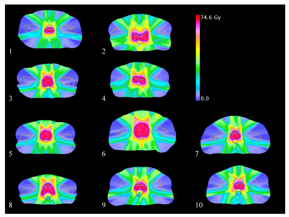
Transverse slices through each PTV center-of-mass slice, showing the final dose distribution after prioritized optimization on all ten cases. Plans were optimized using a quadratic PTV dose slip of 1.0 Gy, and a minimum PTV dose slip of 1.5%. PTV: dark blue; rectum: purple; bladder: light blue; left femur: orange; right femur: tan.

Table 1.

Summary metrics for resulting dose distributions on all ten plans after prioritized optimization using the same slip parameters. Units are Gy except for V40 (in % volume). Performance metrics tend to be very similar, with the exception of plan 2, which appeared to be a lower quality solution (perhaps due to lack of solution optimality).

Plan	D95 to PTV	Min dose to PTV	Standard deviation of PTV dose	Max dose to normal tissues*	Max dose to outer normal tissues**	MOH84 to rectum	V40 to rectum (in %)	Mean dose to bladder
1	67.7	67.6	0.90	68.6	44.1	42.6	44.4	48.6
2	67.7	67.4	0.94	73.2	51.1	54.6	67.4	52.7
3	66.5	65.5	1.38	67.6	55.3	33.5	29.6	26.5
4	67.7	67.5	0.96	69.1	53.1	48.2	52.1	53.3
5	67.8	67.5	0.88	68.7	57.8	30.3	31.0	25.0
6	67.8	67.3	0.92	71.2	59.4	26.9	27.7	25.8
7	67.8	67.7	0.98	68.6	52.7	43.0	45.0	42.3
8	67.8	67.7	0.89	70.3	57.7	46.6	51.3	11.8
9	66.6	65.7	1.30	66.5	54.7	43.6	43.6	39.5
10	67.7	67.2	0.93	69.3	55.0	38.1	35.0	39.0

^*outside of a 0.5 cm range around target

^**outside of a 3.0 cm range around target

Beam weight upper bounds

We found that applying an upper bound to all beam weights (as suggested by Shepard et al.¹²) effectively reduced the possibility of hot-spots away from the target region without degrading target dose distribution quality. To determine this maximum beam weight, we fixed the other parameters at subjectively reasonable values (quadratic slip of 1, min target dose slip of 3%) and looked at a sample case with maximum beam weight ratios (defined as the ratio of maximum beam weight to a beam weight which would deliver the prescription dose if applied to all beams uniformly) of 1, 1.5, 2, 2.5, 3, and 100. Using a value of 1.5 kept hot spots outside the target from getting unreasonably large (larger than about half the target dose), while not restricting the target dosage from achieving excellent target coverage. The corresponding absolute beam weight 1.5 was used for the remaining studies and was found to work well.

Quadratic and minimum PTV dose slip

Having investigated and fixed the above parameters of the optimization, sensitivity to the precise slip factors for the heterogeneity and minimum PTV dose was studied, as further discussed below.

Results

Representative example

Using the tuned optimization parameters, we ran the optimization on all ten cases. The results of a sample case (number 5 out of 10) is examined in more detail in Figure 2 and Figure 3. Note that this case was selected to demonstrate results simply because it has the median value of all ten plans for maximum dose far from the target (outside a 3 cm 3D range around the target).

Figure 2.

Two different transverse slices of a sample case (number 5), showing the dose distribution resulting after using prioritized optimization. PTV: tan, rectum: maroon, left femur: light blue, right femur: pink, bladder: orange.

Figure 3.

Maximum dose projections for case 5. The maximum dose for all slices cumulatively, projected in the transverse, coronal, and sagittal planes. This display demonstrates the lack of unwanted hot-spots away from the target, and corresponding good falloff in all directions away from the target. We found this display (a tool within CERR) to be very useful in capturing plan quality in an approximate yet easily digested fashion.

The mean of the discrete squared Laplacian filter (which approximates the second derivative) for all the beamlets was 99.6, 120.6, 122.2, and 76.4 for steps I through IV, respectively. This shows that the fourth step, which minimizes the sum of the squared beam weights, significantly smoothes beam weights. This is significant because the resulting dose distribution is then more easily (and potentially more accurately) delivered, in fewer beam segments.

Cohort summary

Using a quadratic PTV dose slip of 1.0 and a minimum PTV dose slip of 1.5%, results were obtained which are summarized in Figure 6 and Table 1.

Table 1 shows a summary of the different metrics for each case studied. Note that all plans seem to have similar quality, with the exception of plan 2, which has similar PTV quality but lower quality with respect to the normal tissues. Note, however, that plan 2 did not terminate optimally on any step after the first step. Also, plan 6 appears to do significantly better on the rectum and bladder than the others but these structures had a larger volume compared to the typical cases, which helped reduced the associated dose metrics.

Optimization run times

On average, the optimization (including all four steps) takes 20 minutes. The shortest time was 3 minutes (plan 3) and the longest time was 58 minutes (plan 2). Note that plan 2 exhausted the maximum number of iterations permitted for three of four steps. We add here that the use of hot starts in the optimizer for successive steps (not used in this implementation) may have the potential to significantly decrease this computation time.

Sensitivity to slip values

We carried out several studies designed to document the effect of slip values, and whether target dosimetric tradeoffs were worthwhile, what slip values appeared to be most useful, and how reproducible the effects of slip were.

It is desirable for slip values to yield acceptable PTV minimum doses and target dose homogeneity while reducing as much as possible the dose metrics in the normal structures. In particular, we want slip values which return the “biggest bang for the buck,” allowing the PTV dose distribution to suffer a small amount in exchange for a relatively large gain in lowering dose to normal structures.

Figure 7 shows that slip in the quadratic PTV value does indeed decrease the PTV D95 value, though only by a modest amount (which is apparently manifest near the edge of the PTV). A 1 Gy quadratic slip yields, on average a 2 Gy reduction in D95.

Figure 7.

Average value (over ten plans) of D95 to PTV after running prioritized prescription optimization with various slip values.

From Figure 8, it is apparent that minimum PTV dose slip makes very little difference in the MOH84 to the rectum. In contrast, increased quadratic PTV dose slip either leads to a significant decrease in MOH84 or makes very little difference for others; the effect is plan-specific. The clear trend for the average values is seen in Figure 9. Similar results are seen in Figure 10 as a function of V40.

Figure 8.

MOH84 to rectum (for all ten plans) after running prioritized prescription optimization with various slip values.

Figure 9.

Average value (over ten plans) of MOH84 to rectum after running prioritized prescription optimization with various slip values. The results depend very little on the minimum PTV dose slip value.

Figure 10.

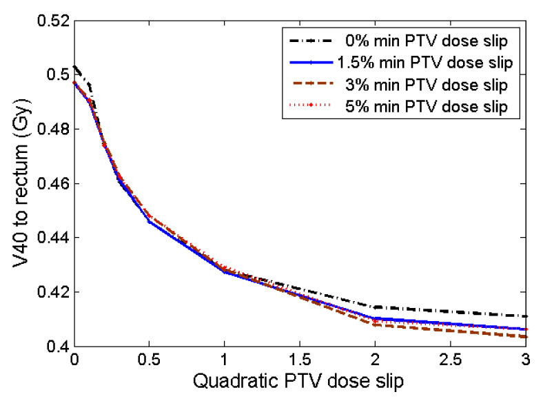
Average value (over ten plans) of V40 to rectum after running prioritized prescription optimization with various slip values. The results correlate closely with MOH84 (in Figure 9), as expected.

The plot lines for V40 and MOH84 (Figure 9 and Figure 10) both have a similar shape, further confirming that MOH84 and V40 seem to be correlated.

The dependence of bladder mean dose on slip is seen in Figure 11. There, in contrast to rectum results, bladder mean dose did depend on minimum PTV slip, when the quadratic PTV slip was large (larger minimum dose slip allowed reduced bladder mean dose).

Figure 11.

Average value (over ten plans) of mean dose to bladder after running prioritized prescription optimization with various quadratic PTV slip values. Note the divergence with respect to minimum PTV dose slip values for higher quadratic PTV slip values.

As shown in Figure 12, maximum doses to normal tissue away from the target edge decreased as quadratic PTV slip increased (except in the case of zero allowed minimum dose slip).

Figure 12.

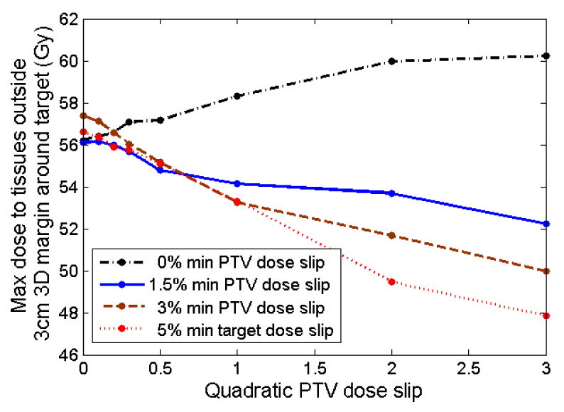
Average value (over ten plans) of maximum dose to normal tissues far from the PTV (outside of a 3 cm 3D region around PTV, within 1.5 cm above and below PTV) after running prioritized prescription optimization with various slip values.

In light of these results, we settled on a quadratic PTV dose slip value of 1.0 Gy and a minimum PTV dose slip of 1.5% as being reasonable, though imperfect operating points.

Discussion and Conclusion

We have demonstrated the application of hierarchical goal programming applied to prostate IMRT planning, dubbed ‘prioritized prescription optimization.’ This was combined with the use of the MOHx (mean-of-hottest x%) objective function for rectal doses to provide for an overall linear/quadratic problem statement.

Formulated in this way, prioritized prescription optimization has several advantages over the traditional method of creating a linearly weighted multi-term objective function, in particular: (1) the physician/planner can enforce more definite choices in how tradeoffs are to be managed prior to treatment planning, (2) the process (once the ‘slip’ factors were determined) is automated, thus freeing the planner to concentrate on final plan evaluation or other important clinical work, (3) objectives which are important, such as beam weight smoothness, but not as important as say, minimum target dose, can be included in later steps without significantly degrading more important objectives, and (4) because normal tissue dosimetric goals are introduced as objective functions (rather than the more conventional method of introducing them as constraints to be met), the planning system attempts to reduce doses to normal tissue structures well as possible without adversely affecting more important goals.

Our motivation to investigate mean-tail-dose objective functions (MOHx or MOCx), as suggested by the Romeijn et al.¹¹, is two-fold: MOHx has a plausible radiobiological interpretation while at the same time being linear and hence computationally attractive. Complication endpoints which are primarily thought to be due to localized ulcerative lesions may be related to the question of whether a large-enough volume or tissue area has been given a large-enough dose. The mean-dose-of-the-hottest x% of a given organ or tissue (x could either be in % or in absolute units of area or volume) thus appears to be a closely related quantity¹⁷. In comparison, more conventional dose volume constraints (“No more than x fractional volume receiving more than y dose”) are also related to this question, but make a more definite, probably unjustifiable, distinction between doses below and above the critical value (y). Moreover, dose-volume constraints introduce non-convex feasibility spaces into the optimization problem, potentially creating multiple local minima and associated issues in solver accuracy and run-time efficiency¹⁵. MOHx may be particularly well-suited as an application to reducing the risk of late rectal bleeding, as there is literature related to the probability of bleeding if the volume (area) receiving a large (> 30 cm² receiving more than 60 Gy¹⁸). The use of mean dose rather than a strict cutoff is consistent with the lack of precise data on this point. In the future, we expect some outcomes studies to be analyzed directly using MOHx (for normal tissues) or MOCx (for tumor response).

The use of mean-tail-dose objective functions does require that the problem size be increased, as discussed by Romeijn et al. For our cases, the problem size increases by approximately 5000 new variables and 5000 new constraints. This was feasible in our case partly because we used a large memory machine (16 GB RAM), and partly because we used somewhat large beamlets (1 cm × 1 cm). One potential strategy for reducing this computational burden is to reduce the spatial sampling for points used to compute MOHx, as suggested by Romeijn et al.¹¹.

Despite using only linear and quadratic objective functions and constraints, we were able to formulate and use outcomes-relevant goals such as MOH84 for the rectum. Using these objective functions, planning time was 20 min on average (without the use of hot starts, which may decrease computation time) on a 2.5 GHz CPU (AMD 64-bit Athlon). Hence, in our view, the use of linear/quadratic objective functions was a success, with the qualification that some plan iterations did not reach optimal termination.

We found that a good strategy for reducing the possibility of hot spots outside the target in addition to reducing large variations in fluence maps is to impose a well-chosen upper limit on the beamlet intensity. Because individual beamlet intensities could be no more than about 1.5 times what would be required to give a uniform prescription dose to the target from all beams, and there are 7 beams, individual beamlets are never hot enough to create undesirable hot-spots far from the target (see Table 1). Moreover, this relatively low level of modulation makes the fluence maps more deliverable. We tested other maximum beamlet bounds and found little degradation on dose from this selection. In fact, the same absolute bound was used and found to be effective for all ten cases.

The goal for step IV was to reduce high-dose regions outside of the target, which had the added benefit of also smoothing the dose. The heuristic of minimizing the sum of the squared beamlet weights smoothes dose outside the target volume, as we demonstrate. The reason is simply that it discourages high-fluence spikes that can lead to hot spots outside the target volume. We tried many alternative objectives for this purpose, including a smoothing function on the fluence map, minimizing the maximum beam weight, minimizing the sum of the beamlet weights, and various objective functions related to dose. The one that we found empirically worked best is minimizing the sum of the squared beamlet weights.

It may be noted that the dose to the femurs is quite low despite it being part of a lower-priority step. In the third step when the mean dose to the bladder, femurs and normal tissue is minimized, the voxels in the bladder and femurs are actually counted twice (because they are also included in the normal tissue). This was intentional, and it results in the dose being diverted from the femurs.

A key imperfection of the current technique is clearly the need to use ‘slip’ factors. As previously noted by others, hierarchical optimization has the disadvantage that it enforces absolute priorities even when the user could potentially ‘give a little to get a lot’ in trading a small relaxation of a higher priority goal for a large improvement in a lower priority goal. We found here, as in the head and neck IMRT study by Wilkens et al.⁴, that in some cases, a small slip in the target dose distribution objective function (especially dose homogeneity) could significantly improve lower priority objective function performance. This was systematized through the use of slip factors. We find here, as for the head and neck IMRT study, that a well-performing set of slip factors can be set for all treatment plans. Thus, slip factors are not factors which need to be tuned by the user of the algorithms, but are rather tuned once-and-for-all.

Despite this, it would nevertheless be desirable to be able to control the tradeoff automatically, so that in cases where little is gained by adding slip (below some threshold), no slip is applied. This is currently a topic of active research in our group.

In summary, we believe that prioritized prescription treatment planning, with some modifications to allow for small but significant tradeoffs between priority levels, combined with linear/quadratic objective functions, provides a powerful, efficient, and relatively automatic tool for IMRT treatment planning for prostate cancer. We conclude that, in principle, IMRTP can be a relatively ‘hands-off’ background process, once the planning problem has been defined. In our view, further testing and refinement of the method for potential clinical use is warranted.

Figure 4.

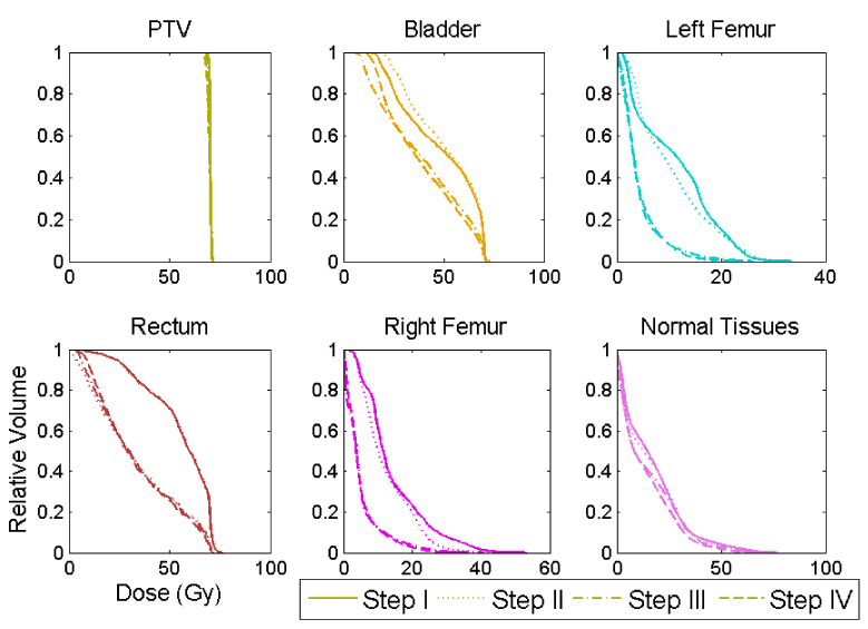
Dose volume histograms after each step of the optimization, for case 5. Note that “Normal Tissues” refers to the area outside of a 0.5 cm 3D region around the PTV, inside of the skin, and within 1.5 cm above and below the PTV. It is easy to see that the rectum is optimized on in step II, whereas the femurs and bladder are introduced in step III. Although there is some degradation in the target DVH, it is small.

Figure 5.

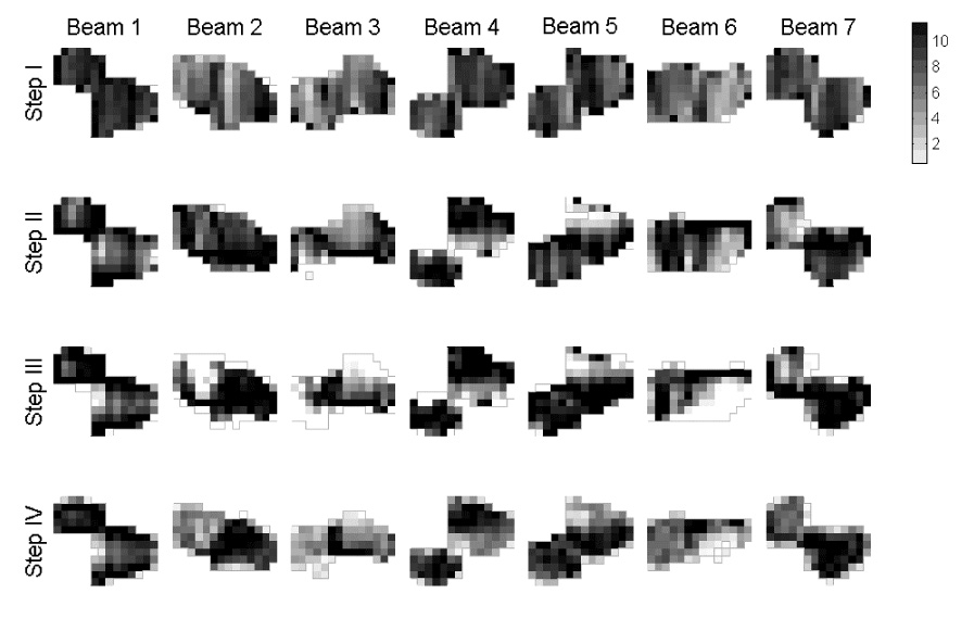
Fluence maps resulting from prioritized optimization for case 5 (arbitrary units). Note how the fields become more limited in Steps II and later as critical tissue avoidance is explicitly incorporated.

References

- 1.Deasy J, Zakaryan K, Alaly JA. Obstacles and advances in IMRT treatment planning. In: Meyer JL, editor. IMRT, IGRT, SBRT: Advances in the Treatment Planning and Delivery of Radiotherapy. San Francisco: Calif.: Karger; 2007. [Google Scholar]
- 2.Craft D, Halabi T, Bortfeld T. Exploration of tradeoffs in intensity-modulated radiotherapy. Phys Med Biol. 2005;50:5857–5868. doi: 10.1088/0031-9155/50/24/007. [DOI] [PubMed] [Google Scholar]
- 3.Craft DL, Halabi TF, Shih HA, et al. Approximating convex pareto surfaces in multiobjective radiotherapy planning. Med Phys. 2006;33:3399–3407. doi: 10.1118/1.2335486. [DOI] [PubMed] [Google Scholar]
- 4.Wilkens J, Alaly JR, Zakaryan K, Thorstad WL, Deasy JO. A Method for IMRT treatment planning based on prioritizing prescription goals. Phys Med Biol. 2006 doi: 10.1088/0031-9155/52/6/009. in press. [DOI] [PubMed] [Google Scholar]
- 5.Deasy JO. Prioritized treatment planning for radiotherapy optimization; CD-ROM Proceedings of the World Congress on Medical Physics and Biomedical Engineering; July 23–28, 2000; Chicago. 2000. p. 4. [Google Scholar]
- 6.Marler RT, Arora JS. Survey of multi-objective optimization methods for engineering. Structural and Multidisciplinary Optimization. 2004;26:369–395. [Google Scholar]
- 7.Min H, Storbeck J. On the Origin and Persistence of Misconceptions in Goal Programming. J Opl Res Soc. 1991;42:301–312. [Google Scholar]
- 8.Charnes A, Cooper WW. Chance-constrained programming. Mgmt Sci. 1959;6:73–79. [Google Scholar]
- 9.Rosenthal R. Principles of multiobjective optimization. Decis. Sci. 1985;16:133–152. [Google Scholar]
- 10.Romeijn HE, Ahuja RK, Dempsey JF, et al. A new linear programming approach to radiation therapy treatment planning problems. Operations Research. 2006;54:201–216. [Google Scholar]
- 11.Romeijn HE, Ahuja RK, Dempsey JF, et al. A novel linear programming approach to fluence map optimization for intensity modulated radiation therapy treatment planning. Physics in Medicine and Biology. 2003;48:3521–3542. doi: 10.1088/0031-9155/48/21/005. [DOI] [PubMed] [Google Scholar]
- 12.Shepard DM, Ferris MC, Olivera GH, et al. Optimizing the delivery of radiation therapy to cancer patients. Siam Review. 1999;41:721–744. [Google Scholar]
- 13.Deasy JO, Blanco AI, Clark VH. CERR: a computational environment for radiotherapy research. Med Phys. 2003;30:979–985. doi: 10.1118/1.1568978. [DOI] [PubMed] [Google Scholar]
- 14.Deasy J, Lee E, Bortfeld T, Langer M, Zakarian K, Alaly J, Zhang Y, Liu H, Mohan R, Ahuja R, Pollack A, Purdy J, Rardin R. A collaboratory for radiation therapy treatment planning optimization research. Ann Op Res. 2006 in press. [Google Scholar]
- 15.Deasy JO. Multiple local minima in radiotherapy optimization problems with dose-volume constraints. Medical Physics. 1997;24:1157–1161. doi: 10.1118/1.598017. [DOI] [PubMed] [Google Scholar]
- 16.Deasy JO, Fowler JF. The Radiobiology of Intensity Modulated Radiation Therapy. In: Mundt AJ, Roeske J, editors. Intensity Modulated Radiation Therapy: A Clinical Perspective. Hamilton, Ontario: BC Decker; 2005. pp. 53–74. [Google Scholar]
- 17.El Naqa I, Clark VH, Chen Y, Vicic M, Khullar D, Shimpi S, Hope A, Bradley J, Deasy JO. Treatment Outcome-based Objective Functions for IMRT Treatment Planning (abstr.) Int J Radiat Oncol Biol Phys. 2006;66:S687–S688. [Google Scholar]
- 18.Fenwick JD, Khoo VS, Nahum AE, et al. Correlations between dose-surface histograms and the incidence of long-term rectal bleeding following conformal or conventional radiotherapy treatment of prostate cancer. Int J Radiat Oncol Biol Phys. 2001;49:473–480. doi: 10.1016/s0360-3016(00)01496-6. [DOI] [PubMed] [Google Scholar]