

Abstract
We have investigated 3-dimensional brain current density reconstruction (CDR) from intracranial electrocorticogram (ECoG) recordings by means of finite element method (FEM). The brain electrical sources are modeled by a current density distribution and estimated from the ECoG signals with the aid of a weighted minimum norm estimation algorithm. A series of computer simulations were conducted to evaluate the performance of ECoG-CDR by comparing with the scalp EEG based CDR results. The present computer simulation results indicate that the ECoG-CDR provides enhanced performance in localizing single dipole sources which are located in regions underneath the implanted subdural ECoG grids, and in distinguishing and imaging multiple separate dipole sources, in comparison to the CDR results as obtained from the scalp EEG under the same conditions. We have also demonstrated the applicability of the present ECoG-CDR method to estimate 3-dimensional current density distribution from the subdural ECoG recordings in a human epilepsy patient. Eleven interictal epileptiform spikes (seven from the frontal region and four from parietal region) in an epilepsy patient undergoing surgical evaluation were analyzed. The present promising results indicate the feasibility and applicability of the developed ECoG-CDR method of estimating brain sources from intracranial electrical recordings, with detailed forward modeling using FEM.
Keywords: finite element method, current density reconstruction, electrophysiological neuroimaging, brain source imaging, EEG, ECoG, intracranial recordings, interictal spike, epilepsy
I. Introduction
Information on the locations of electrical activity in the brain is of interest and importance for neuroscience research and clinical applications in aiding diagnosis and surgical planning of neurological diseases. The electroencephalography (EEG) is a measurement of the electrical activity of the brain by recording from electrodes placed on the scalp. Due to the fact that EEG is convenient, noninvasive, safe and inexpensive, significant efforts have been devoted to exploration of locations of brain source activity based on the scalp-recorded EEG signals by solving the so-called EEG inverse problem. These EEG (or MEG, magnetoencephalography) inverse solutions may be classified into two major categories according to the difference between source models (He & Lian, 2002, 2005): equivalent dipole localization (Scherg et al, 1985; He et al 1987; Hämäläinen & Sarvas, 1989; Mosher et al 1992, 1999; Cuffin 1995; Leahy et al, 1998; Merlet et al, 2001; Xu et al, 2004; Ding et al, 2007) and distributed source imaging (Hämäläinen et al, 1984, 1994; Dale & Sereno, 1993; Gevins et al, 1994; Nunez et al, 1994; Pascual-Marqui et al, 1994, 1995, 1999; He et al, 1996, 1999, 2001, 2002a, 2002b, 2002c; Babiloni et al, 1997, 2003, 2005; Phillips et al, 1997; Wang & He, 1998; Fuchs et al, 1999; Grave et al, 2000; Liu et al, 2006, 2008; Astolfi et al, 2007a, 2007b; Ding & He, 2007). But all of these EEG based inverse solutions suffer from the low signal-to-noise ratio (SNR) because EEG signals are recorded by sensors physically separated from the cortex by the skull which blocks and smoothes the potential field recorded on the scalp.
The electrocorticogram (ECoG) recorded from multi-contact subdural electrodes implanted during surgical evaluation in epilepsy patients provides higher SNR and temporal and spatial resolution than EEG due to the fact that ECoG signals are not influenced by the low conductivity skull and are recorded in the vicinity of the underlying brain sources. In clinical practice, the ECoG has become the “gold standard” for defining epileptogenic zones (Engel et al, 1981). Usually, the planning of ECoG grids implantation is determined using clinical data: ictal features, scalp EEG and structural MRI findings (Bénar et al, 2006). The pattern of the ECoG recordings is then used for localization purposes. However, the ECoG measurements sometimes still remain ambiguous in localizing source signals arising from deep regions, such as sulcal fundi.
In order to improve the localization accuracy of the brain source estimation methods, several investigators have tried to estimate the neural activity locations based on the intracranial ECoG recordings. Towle and his co-workers (Towle et al, 2003) performed dipole source localization from subdural somatosensory evoked potential (SEP) recordings in five patients and found that the dipole analysis agreed with conventional interpretation of SEP waveform inversion and had the advantage of providing localization to a single point which was quantitatively compared to the noninvasive test results. They used a simple single-shell spherical epicortical model in their study and did not consider the effects of the scalp, skull, cerebrospinal fluid (CSF) and the implanted ECoG strips. Korzyukov et al (Korzyukov et al, 2007) applied the distributed source imaging approach to the intracranial P50 response of auditory evoked potentials and the gating difference wave to do source localization by using the LORETA algorithm (Pascual-Marqui et al, 1994). Their aim was to study the cortical mechanisms underlying auditory sensory gating and no detailed analysis of the performance of the brain source estimation method was described. Korzyukov and co-wokrers used the boundary element method (BEM) based head model consisting of the scalp, skull and brain compartments without considering the effect of implanted ECoG grids and CSF. Fuchs et al (2007) studied the performance of the spherical and realistically shaped BEM volume conductor models for EEG and ECoG source reconstruction in spherical and non-spherical parts of the head with simulations and measured epileptic spike data. They investigated the accuracy and efficiency of three numerical methods, i.e. standard boundary element method (sBEM), interpolated boundary element method (iBEM) and interpolated finite element method (iFEM), in EEG forward/inverse solutions. In Fuchs et al.’s study (2007), their ECoG based brain source imaging studies were all based on the simple single-layer BEM model consisting of the brain, and non-insulating conductive medium surrounding the brain was ignored.
In the present study, we investigate 3-dimensional (3D) current density reconstruction (CDR) to estimate brain sources from the intracranial ECoG recordings by using the finite element method based on the complex realistic geometry head model built from the patient’s specific magnetic resonance (MR) and computer tomography (CT) image data. Our ECoG based current density reconstruction (ECoG-CDR), for the first time to our knowledge, considers the effects of the scalp, skull, CSF, brain and the implanted ECoG base pads by using the FEM technique to avoid the boundary condition changes and the lead field distortions in the head volume conductor modeling. Performance analysis and evaluation of the present ECoG based CDR (ECoG-CDR) were performed by comparing it with the conventional 3D CDR from the scalp EEG recordings (EEG-CDR) in a series of computer simulations. The ECoG-CDR was also applied to real data during interictal spikes in a human epilepsy patient.
II. Methods
1. Source Model and Geometry Model
The equivalent dipole source model and the distributed source model are two types of source models commonly used in brain source localization. Compared with the extracranial EEG measurement, the intracranial ECoG recording is a kind of near-field measurement thus the distributed source model was used in the present study. We assumed that the current dipoles are distributed over a fixed lattice covering the 3D brain volume with the inter-grid distance of 6 mm and the three orthogonal dipole components of the Cartesian coordinate system at each node represent one dipole moment at that location.
The realistic geometry FEM head model consisting of the scalp, skull, CSF, brain and two silastic ECoG base pads (the 8×8 parietal ECoG pad was 80×80 mm while the 8×4 frontal ECoG pad was 80×40 mm) was built from a human subject’s MR and CT image data by using a protocol which we have previously described (Zhang et al., 2006a). Note that, in clinical setting, the subdural ECoG electrodes are usually embedded in the silastic base pad with a thickness of around 2 mm. The ECoG base pads and CSF layer are the two parts in our head model whose thickness is relatively small compared with the other parts. We modeled the ECoG base pads and CSF layer in our FEM model using the tetrahedrons with the element size of around 3 mm, and modeled the other tissues in the FEM model using the tetrahedrons with the element size of around 6 mm. The overall average length of the finite elements in our whole FEM model was around 5 mm and the whole FEM model consisted of 84,888 tetrahedron elements and 15,407 nodes. It is worthy to note that part of brain elements which are close to the brain-to-CSF boundary, i.e. cortical surface, were also meshed with the 3 mm-length tetrahedrons, and the other brain element lengths increase gradually as they go far away from the cortical surface. The purpose of this adaptive meshing operation is to avoid the size jump between the neighboring elements which will cause numerical errors. We used this local refined FEM meshing technique to build the FEM model in order to decrease the computational loads while maintaining satisfactory computational accuracy. Note also that the slightly increased thickness of model of the CSF layer and ECoG base pads is based on numerical consideration in order to achieve a robust solution. The conductivities of the scalp and brain were set to 0.33 s · m−1, the conductivity of the skull was set to 1/20 of the conductivity of the brain, 0.0165 s · m−1 (Zhang et al., 2006b), the conductivity of the CSF was set to 1.0 s · m−1 and the conductivity of the silastic ECoG grids was set to 3.3e-11 s · m−1.
2. Forward Solver
The brain electric forward problem is considered as follows: given the positions and moments of the current dipole sources and the geometry and electrical conductivity profile of the volume conductor, i.e. the head, calculate the electrical potentials within the head volume conductor. Theoretically, this problem can be stated by Poisson's equation which is defined on the volume conductor, Ω, (Gulrajani, 1998) and the Neumann boundary conditions on the scalp, S:
| (1) |
where σ is the conductivity tensor which is a function of the location within the volume conductor, n is the outward unit normal to the scalp S, and Is the volume current densities due to the presence of the current sources. The unknown, ϕ, is the electrical potential generated by current sources. Generally, s at each location is different from other locations with a certain level of discrepancy. Such discrepancy is assumed to be small and negligible within each of the main structures of human head, i.e. the scalp, skull, brain, and CSF, which leads to the layered volume conductor model widely adopted in the brain electric forward modeling (Rush et al, 1969, He et al, 1987, 1999, 2002c; Hämäläinen & Savars, 1989; Mosher et al., 1999; Finke et al., 2003).
In the present study, the brain electric forward solution was obtained based on the realistic geometry multi-compartment head model described above by means of FEM. In this case, Poisson’s equation was transformed into a group of linear equations defined on the nodes of the finite element model and the equation was formulated in a matrix form as follows (Zhang et al., 2004).
| (2) |
where K is the stiffness matrix which incorporates the volume conductor model information, e.g. geometry and conductivity, Φ is the potential vector on the finite element nodes, G is the load matrix due to the current sources and is decided by the current source and the geometry and conductivity information of the element where the current source is located. The linear finite element was used to implement the finite element method in the present study. The linear problem stated as equation (2) was solved by a linear solver, i.e., the preconditioned conjugate gradients method (Silvester et al, 1996) and the electrical potential value on every node in the FEM model was obtained.
3. Transfer Matrix Construction
The linear relationship between the source space and the measurement space can be expressed as:
| (3) |
Where Φ = (ϕ1,ϕ2,…,ϕM)T is the vector of measurements, X = (x1,x2,…,x3×N)T is the vector representing the strength of the distributed dipoles in the 3D brain tissue space, T is the transfer matrix between Φ and X and n is the noise vector. M refers to the number of recording electrodes in the measurement space and N refers to the number of current dipole sources within the entire solution space. In 3D current density reconstruction methods, the number of total unknown dipole components is 3 × N because the three orthogonal components represent one dipole moment at each location.
For our present 3D ECoG-CDR method, equation (3) can be rewritten as:
| (4) |
where Φi represents the vector of measurements on the intracranial ECoG grids and Ti represents its corresponding transfer matrices. In the present study, the numbers of ECoG electrodes are 64, 78 and 96, respectively.
Assuming only one dipole in the source space is active with unit strength in one of the three orthogonal directions and both the components in the other directions and the other dipoles in the source space are zero, the potential field corresponding to each component of each current dipole in the source space can be obtained by iteratively solving equation (4). Φi for each dipole source can then be separated from the entire solution and the lead field matrix relating the dipoles in the source space and the intracranial ECoG potential field can thus be formed column by column, denoted as Ti. Similarly, the lead field matrix relating the dipoles in the source space and the extracranial EEG potential field can be obtained in the same fashion, denoted as Te in the following equation:
| (5) |
In the present study, 128 scalp EEG electrodes were used in the computer simulation. Fig. 1(b) shows the distribution of the scalp EEG electrodes used.
Fig. 1.
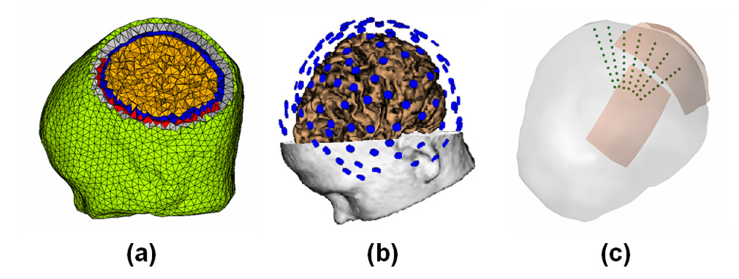
The complicated finite element model, EEG electrodes configuration and dipole configurations in the computer simulations. (a) The finite element model consisting of the brain (green), skull (gray), CSF (blue), brain (yellow) and silastic subdural ECoG grid (red); (b) 128 scalp EEG electrodes configuration; (c) 7 dipole groups used in the computer simulations.
4. Inverse Solver
Generally, equation (3) or equation (4) and equation (5) are underdetermined problems because the number of measurements is less than the number of sources. The minimum-norm regularization was used to obtain a unique solution, and can be expressed by the following equation by taking equation (3) as an example.
| (6) |
The first term of the objective function is the error term in the least squares sense and the second term is the regularization term which attempts to minimize the total energy of the solution. λ is the regularization parameter which was determined by means of the L-curve method (Hansen, 1992).
The weighted minimum-norm regularization (Pascual-Marqui et al., 1994; Philips et al, 1997; Fuchs et al., 1999) was applied in the present ECoG-CDR to account for the undesired depth dependency. The objective function (6) is transformed to the following equation:
| (7) |
where W is a diagonal matrix with elements determined from the lead field matrix T.
5. Simulation Protocols
Computer simulations were conducted to evaluate the performance of the present ECoG-CDR method. The FEM head model described above was used in all computer simulations, shown in Fig. 1(a). Seven groups of dipole locations were considered in the computer simulations, shown in Fig. 1(c). Every dipole group consisted of 10 dipoles evenly placed from 5 mm to 50 mm below the cortical surface. The 1st dipole group was placed below the center of the parietal ECoG grid and the 2nd group was placed 10 mm away from the center of the parietal grid (measured by the distance between the shallowest dipole location in the 1st dipole group and the center of the ECoG grid). Similarly, the 3rd dipole group was placed 20 mm away from the center of the parietal grid, and so on. A total of 7 dipole groups were placed in this manner. Notice that the 5th dipole group, which is placed 40 mm away from the center of the parietal ECoG grid, was exactly below the edge of the grid. We designed this source configuration to investigate the performance of the present ECoG-CDR method for the brain sources with different locations relative to the location of the ECoG grids.
In our computer simulations, one current dipole in one dipole configuration was considered at a time to investigate the accuracy of 3D ECoG-CDR by comparing it with the EEG-CDR, in which the FEM head model without silastic ECoG grids was used. Two current dipoles in two dipole different dipole groups with the same source depth were also considered in order to investigate the effects of multiple sources on the spatial resolution of the present ECoG-CDR method. At each dipole location, both radially and tangentially oriented dipoles were considered. The radial and tangential directions were defined by the local curvature of the point on the cortical surface which was closest to the simulated dipole source. Gaussian white noise (GWN) of 5–20% (SNR 20 to 5), which is defined as the ratio between the standard deviation of the noise and the root mean square of the potential, was used to simulate the noise-contaminated recording environment. Furthermore, the effect of the number of subdural ECoG electrodes on the ECoG-CDR results was also assessed by using 64 (from the parietal ECoG grids), 78 (in which 32 electrodes from the frontal ECoG grid and 46 from the parietal grid were used) and 96 electrodes (all of the electrodes from the frontal and parietal grids).
The localization error, which is defined as the distance between the simulated source location and reconstructed source location, was calculated and used to assess the performance of the ECoG-CDR in the present study. The reconstructed source point is defined as the center of the current density distribution, which is calculated as the geometry center of all the grids on which the reconstructed current density strengths are over a 70% threshold of the maximum current density.
6. Data Collection in an Epilepsy Patient
The ECoG data from a 12 year old female epilepsy patient was collected according to a protocol approved by the Institutional Review Boards (IRBs) of the University of Minnesota and the University of Chicago. Two standard subdural electrode grids were used in this patient: the parietal grid contained 64 (8 × 8) platinum contacts in a rectangular array with a 10 mm center-to-center spacing and the frontal grid consisted of 32 (4×8) platinum contacts with the same 10 mm center-to-center spacing. The platinum disks were embedded in a silastic base and had an exposed surface diameter of 2.3 mm. Continuous recordings from the subdural channels (i.e. 46 electrodes from the 8×8 grid and 32 from the 4×8 grid) were obtained by using BMSI6000 (Nicolet Biomedical, Madison, WI). The data were measured with a frequency bandwidth of 1–100 Hz and sampled at a rate of 400 Hz. Intra-cranial electrode positions were determined using postoperative CT image.
Interictal epileptiform spikes were selected from the recorded ECoG signals and analyzed to evaluate the present ECoG-CDR method. The reconstructed ECoG-CDR results were qualitatively (via visual inspection) compared to the locations of the foci as determined by the epileptologist.
III. Results
1. Comparison between the ECoG-CDR and the EEG-CDR in the case of a single dipole source
Fig. 2 shows the typical tomography of the strengths of the current sources estimated in the 3D solution space by means of the present ECoG-CDR method. This particular example was created using the 3rd dipole in the 1st dipole group as previously described in the “Simulation Protocols” section. Figs.2 (a), (b) and (c) show the ECoG-CDR results using three different visual angles, respectively. Capital L and R around the axial and coronal view sub figures indicate left and right directions respectively, and the directions of all the axial and coronal view figures in the present study are shown in the same way with Fig. 2. The localization error for this case was 2.87 mm.
Fig. 2.
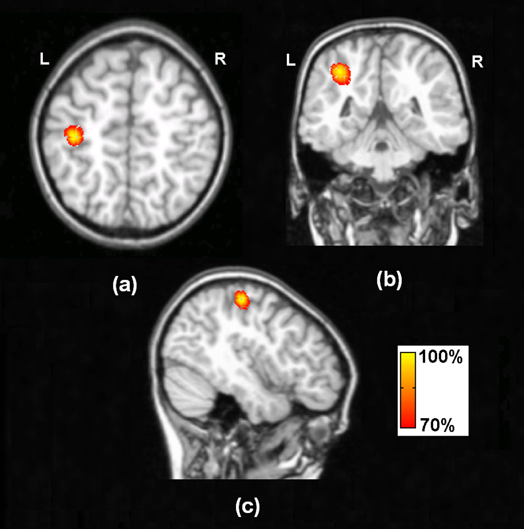
Typical tomography of the strengths of the current sources estimated by the present ECoG-CDR method using the unit radial dipole at the 3rd dipole location in the 1st dipole group, the dipole source depth is 15mm.
Fig.3 compares the accuracy of the ECoG-CDR and the EEG-CDR in terms of the localization error. Ten trials of 5% (SNR 20) GWN were generated and the mean and standard deviation of the ECoG-CDR and EEG-CDR methods were evaluated. Figs. 3 (a), (b), (c), (d), (e), (f) and (g) respectively show the comparison results from the dipole group #1, #2, #3, #4, #5, #6 and #7 in the dipole configuration shown in Fig. 1(c). The upper panels and lower panels refer to tangential and radial dipole being used in the simulation. From Fig. 3 we can see the following phenomena: (1) For any dipole group, covered or not covered by the ECoG grids, the overall trend of the localization error curves calculated by either the ECoG-CDR or the EEG-CDR is that the localization error increases as the dipole source depth increases. This phenomenon is consistent with the previous literature (Ding et al, 2005). (2) For the dipole groups which are covered by the ECoG grids, i.e. the 1st, 2nd, 3rd and 4th dipole groups, most of the results from the present ECoG-CDR (blue solid line) show better accuracy than the results from the EEG-CDR (red dashed line). Exceptions are the 9th and 10th dipole sources in the 2nd dipole group with tangential dipole moments, the 10th dipole source in the 3rd dipole group with radial dipole moments, and the 10th dipole source in the 4th dipole group with both radial and tangential dipole moments. This shall be due to the fact that the dipole is far away from the subdural ECoG electrodes. (3) For the dipole groups which are not covered by ECoG grids, i.e. the 6th and 7th dipole groups, the EEG-CDR (red dashed line) shows better current density reconstruction results than the ECoG-CDR (blue solid line). This shall be due to the fact that the dipoles are far away from the subdural ECoG electrodes. (4) For the dipole groups located exactly below the edge of the ECoG grids, i.e. the 5th dipole group, the current density estimation results from the ECoG-CDR exhibit a fair amount of instability while the EEG-CDR produces results with accuracy as robust as the other dipole configurations.
Fig. 3.
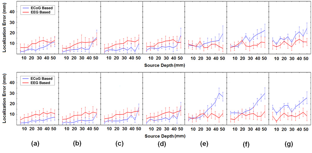
Comparison between the ECoG-CDR and the EEG-CDR in the case of a single dipole source. The subfigures (a), (b), (c), (d), (e), (f) and (g) respectively show the comparison results from the dipole group #1, #2, #3, #4, #5, #6 and #7 in the dipole configuration shown in Fig. 1(c), and every subfigure include one upper panel figure and one lower panel figure in which the united tangential and radial dipole moment are used in the comparison. In every subfigure, the horizontal axis refers to the depth of dipole from the cortical surface. The vertical axis indicates the localization error (mm) and the solid curves and the vertical dashed lines depict the change of the mean localization error and the standard deviation, respectively, as the dipole source depth changes from 5 mm to 50 mm below the cortical surface. The blue dashed and the corresponding vertical lines depict the results obtained by using the present ECoG-CDR method, and the red solid and the corresponding vertical lines depict the results obtained by using the EEG-CDR method.
2. Influence of noise level
The 3rd dipole location in the 1st dipole group was selected to investigate the influence of noise level on the accuracy of the present ECoG-CDR method. Gaussian white noise with different noise levels was added to the simulated ECoG potentials produced by the above-mentioned dipole. The changes in the localization error caused by varying the noise level from 5% to 20% (SNR 20 to 5) are shown in Fig. 4. Note that in all conditions, the localization errors increase when the noise level increases.
Fig. 4.
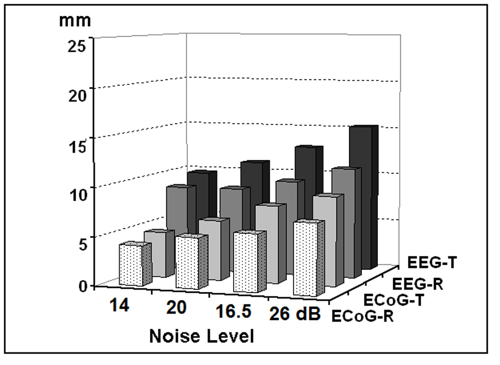
Localization errors of the present ECoG-CDR and the traditional CDR methods at different noise levels, by taking the 3rd dipole location in the 1st dipole group with radial and tangential dipole moment. The physical unit of vertical axis is mm. “EEG-R” refers to the results obtained by using the EEG based reconstruction method when dipoles are oriented in radial direction. “EEG-T” refers to the results obtained by using the EEG based reconstruction method with tangential dipole. “ECoG-R” and “ECoG-T” refer to the results obtained by using the ECoG based reconstruction method with radial and tangential dipole, respectively.
3. Influence of electrode number
Fig. 5 depicts the localization error with different numbers of intracranial ECoG electrodes by using the 3rd dipole location in the 1st dipole group. Three electrode numbers, i.e. 64, 78 and 96, were used in this simulation. The 96-electrodes configuration includes 64 electrodes from the parietal grid and 32 electrodes from the frontal grid; the 78-electrodes configuration includes 32 electrodes from the frontal grid and 46 electrodes from the parietal grid; and the 64-electrodes configuration includes 64 electrodes from the parietal grid.
Fig. 5.
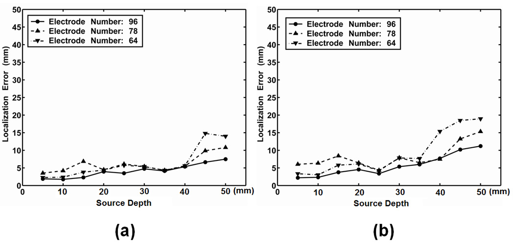
Influence of the ECoG electrodes number on the localization errors of the present ECoG-CDR method, by taking the 1st dipole group. (a) Radial dipole, (b) Tangential dipole. The horizontal axis refers to the dipole depth from the cortical surface and the vertical axis refers to the source localization error.
It is observed that the electrode number has little influence on the ECoG-CDR accuracy in term of localization error for the shallow source depths (above 40 mm) although a slight decrease of localization error can be noticed as the number of electrodes increases.
4. Comparison between the ECoG-CDR and the EEG-CDR in the case of multiple dipole sources
Fig. 6 shows the tomography of the strengths of the current sources produced by two separate dipole sources (one from the 1st dipole group and the other from the 3rd or the 4th dipole group with the same source depth as the 1st one), with a threshold set at 70% of the maximum current density. The performance of the ECoG-CDR and the EEG-CDR with multiple dipole sources was compared using this dipole configuration. The 5 subfigures in the 1st row (from (a1) to (a5)) show the results from the ECoG-CDR with source depths of 10 mm, 15 mm, 20 mm, 25 mm and 30 mm and inter-source distances of 19.4 mm, 18.5 mm, 17.6 mm, 16.8 mm and 16.0 mm respectively. Note that the difficulty in the ability to distinguish the separate sources in these 5 cases increases as the inter-source distance decreases and the source depth increases. We can see that the ECoG-CDR can clearly distinguish two closely separate dipole sources when the inter-source distance is as small as 16.8 mm and the source depth is 25 mm, shown in (a4). For deeper and closer dipole source configuration, i.e. (a5) with a source depth of 30 mm and inter-source distance of 16.0 mm, the present ECoG-CDR method is unable to resolve two separate sources. The 2 subfigures in the 3rd row ((c1) and (c2)) show the results from the EEG-CDR with a source depth of 10 mm and 15 mm and intersource distance of 19.4 mm and 18.5 mm. The dipole configurations for the subfigures in the 3rd row are consistent with the first 2 subfigures in the 1st row in order to compare the performance between the ECoG-CDR and the EEG-CDR. We can see that the EEG-CDR can clearly distinguish two close separate dipole sources with an inter-source distance of 19.4 mm at a depth level of 10 mm as shown in (c1), but it cannot differentiate deeper and closer dipole source pairs to the same extent as the ECoG-CDR. To further test the EEG-CDR’s ability to distinguish the multiple dipole sources, we enlarged the inter-source distance and applied the EEG-CDR again, results of which are shown in the 4 subfigures in the 2nd row of Fig. 6. The source depths, from left to right, are still set to 10 mm, 15 mm, 20 mm and 25 mm, but the inter-source distances in the multiple dipole configurations are enlarged to 29.1 mm, 27.8 mm, 26.5 mm and 25.2 mm. Under these conditions, the EEG-CDR was only able to distinguish sources separated by a minimum of 27.8 mm at a depth of 15 mm.
Fig. 6.
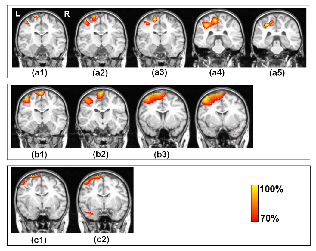
Comparison between the present ECoG-CDR and the EEG-CDR methods in the case of multiple dipole sources. The 1st row (from (a1) to (a5)) show the tomography of the strengths of the current sources estimated by using the present ECoG-CDR with the dipole source pairs in which one dipole source comes from the 1st dipole group and the other one comes from the 3rd dipole group with the same source depth, the source depths are 10 mm, 15 mm, 20 mm, 25 mm and 30 mm and inter-source distances are 19.4 mm, 18.5 mm, 17.6 mm, 16.8 mm and 16.0 mm, respectively. The 2nd row (from (b1) to (b4)) show the tomography of the strengths of the current sources estimated by using the EEGCDR with the dipole source pairs in which one dipole source comes from the 1st dipole group and the other one comes from the 4th dipole group with the same source depth, the source depths are 10 mm, 15 mm, 20 mm and 25 mm, and the inter-source distances are 29.1mm, 27.8mm, 26.5mm and 25.2mm respectively. The 3rd row ((c1) and (c3)) show the tomography of the strengths of the current sources estimated by using the EEG-CDR with the dipole source pairs in which one dipole source comes from the 1st dipole group and the other one comes from the 3rd dipole group with the same source depth, the source depths are 10 mm and 15 mm and inter-source distances are 19.4 mm and 18.5 mm, respectively. All the dipole sources used in this figure are in radial direction.
5. Imaging interictal sources in an epilepsy patient using the ECoG-CDR
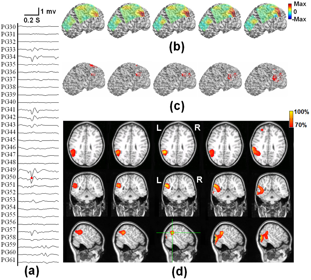
Fig. 7 shows the locations of subdural ECoG electrodes implanted in an epilepsy patient undergoing surgical evaluation. Red circles refer to the electrodes which are considered to be ictal onset zone based on clinical evaluation of the ictal ECoG recordings. Fig. 8 shows the 3D current density estimation results in an epilepsy patient from a frontal interictal spike, by means of the ECoG-CDR. In total, maps of five time points (two time points before and after the spike peak, as well as the time point at the peak itself) with a time separation of 2.5 ms between points are depicted. Figs. 8 (a) shows the ECoG recordings measured directly from the frontal and parietal grids, and (b) displays the potential maps of the ECoG recordings which were normalized to the maximal absolute value of the entire ECoG recordings over the frontal and parietal grids. Note that the major activity of the ECoG recordings occurs on the frontal grid and the maximal activity occurs at the peak of the interictal spike. Fig. 8 (c) shows the reconstructed current density distribution obtained by using the present ECoG-CDR method, where all the points on which the reconstructed current density strength is over a 70% threshold of the maximum current density strength are displayed in red color in the 3D space closed by the semitransparent cortical surface. The subfigure rows from top to bottom in Fig. 8 (d) respectively shows the axial, coronal and sagittal views of the strengths of the estimated current density obtained by using the ECoG-CDR, the green lines on the sagittal slice at interictal spike peak instant indicate the location of the axial and coronal views, and all the angle views at other interictal spike instants share the same cut locations with those at the peak instant. Note that the estimated 3D current density has a centralized distribution and highest resolution at the peak point of the interictal spike, and also with the maximal current strength according to the color bar on the top right corner. The current density distribution becomes smooth, the resolution decreases, and the maximal current strength decreases at the same time as the estimation instant moves further from the peak point.
Fig. 7.
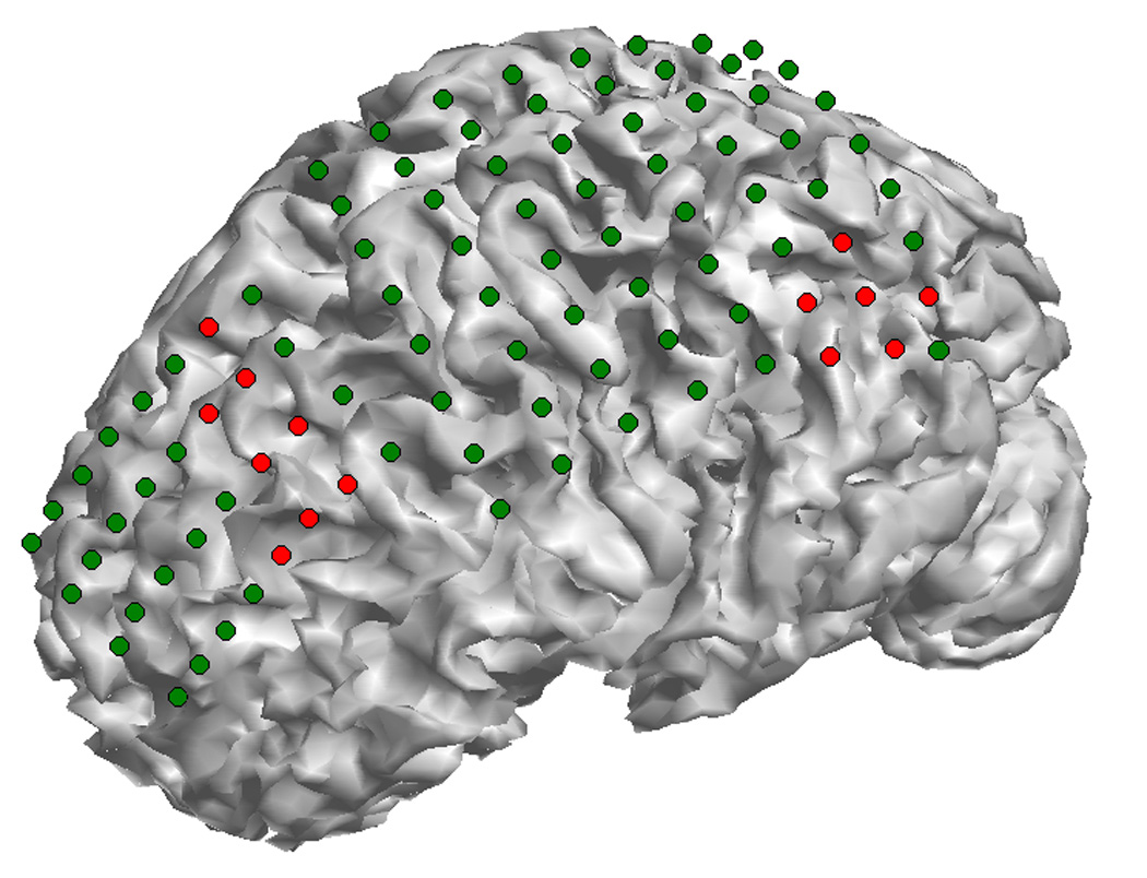
The epileptogenic zones of the epilepsy patient as identified from ictal ECoG recordings. The dots on the cortical surface show the ECoG grids segmented from CT images, and the red ones show the epileptogenic zones. Two ictal onset zones were identified in this patient: one is located at the left parietal lobe and the other one is located at the anterior frontal lobe.
Fig. 8.
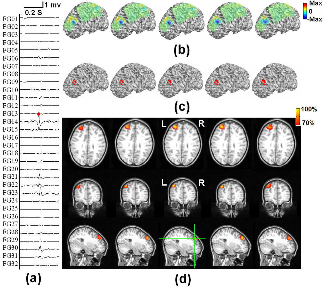
The tomography of the strengths of the current sources estimated by using the present ECoG-CDR method at different time points during an interictal spike at the anterior frontal lobe of a pediatric epilepsy patient, from 5 ms before and 5 ms after the peak of the spike. (a) The ECoG recordings measured directly from the frontal and parietal grids. (b) The potential maps of the ECoG recordings which were normalized to the maximal absolute value of the entire ECoG recordings over the frontal and parietal grids. (c) The reconstructed current density distribution obtained by using the present ECoG-CDR method in the 3-dimensional space with a threshold set at 70% of the maximum current density value. (d) The axial, coronal and sagittal views (from top to bottom row) of the strengths of the estimated current density, the green lines on the sagittal slice at interictal spike peak instant indicate the location of the axial and coronal views.
Fig. 9 shows the 3D current density estimation results of the same epilepsy patient from a parietal interictal spike using the ECoG-CDR. Similarly, maps at five time points (two time points before and after the spike peak as well as the time point at the peak itself) with a time separation of 2.5 ms between the points are depicted. Figs. 9 (a) shows the ECoG recordings measured directly from the parietal and frontal grids, and (b) displays the potential maps which were normalized to the maximal absolute value of the entire ECoG recording over the frontal and parietal grids. In this case, the major activity of the ECoG recording occurs on the parietal grids and the maximal activity occurs at the peak point of the interictal spike. Fig. 9 (c) shows the reconstructed current density distribution obtained by using the ECoG-CDR in the 3D space with a threshold set at 70% of the maximum current density value. Fig. 9 (d) shows an axial, coronal and sagittal views (from top to bottom row) of the strengths of the estimated current density, the green lines on the sagittal slice at the interictal spike peak instant indicate the location of the axial and coronal views. A similar phenomenon as seen in Fig. 8 can also be found in Fig. 9 in which the estimated 3D current density has a centralized distribution with a highest resolution at the peak of the interictal spike and the current density distribution becomes smooth and the resolution decreases as the estimation moves further from the peak point.
Fig. 9.
The tomography of the strengths of the current sources estimated by using the present ECoG-CDR method at different time points during an interictal spike at the left parietal lobe of a pediatric epilepsy patient, from 5 ms before and 5 ms after the peak of the spike. (a) The ECoG recordings measured directly from the frontal and parietal grids. (b) The potential maps of the ECoG recordings which were normalized to the maximal absolute value of the entire ECoG recordings over the frontal and parietal grids. (c) The reconstructed current density distribution obtained by using the present ECoG-CDR method in the 3-dimensional space with a threshold set at 70% of the maximum current density value. (d) The axial, coronal and sagittal views (from top to bottom row) of the strengths of the estimated current density, the green lines on the sagittal slice at interictal spike peak instant indicate the location of the axial and coronal views.
Fig. 10 shows an axial view of the strengths of the estimated current density obtained by using the ECoG-CDR from 9 other interictal spikes (6 frontal and 3 parietal spikes). Comparing this result to the ictal foci as determined by the epileptologist (frontal electrodes: 5, 6, 7, 14, 15, 22, 23 and 31, parietal electrodes: 42, 49, 50, 51, 58 and 59), shown in Fig. 7, the estimated brain activity in the 3D space by using the ECoG-CDR is consistent with the patient’s clinical diagnosis.
Fig. 10.
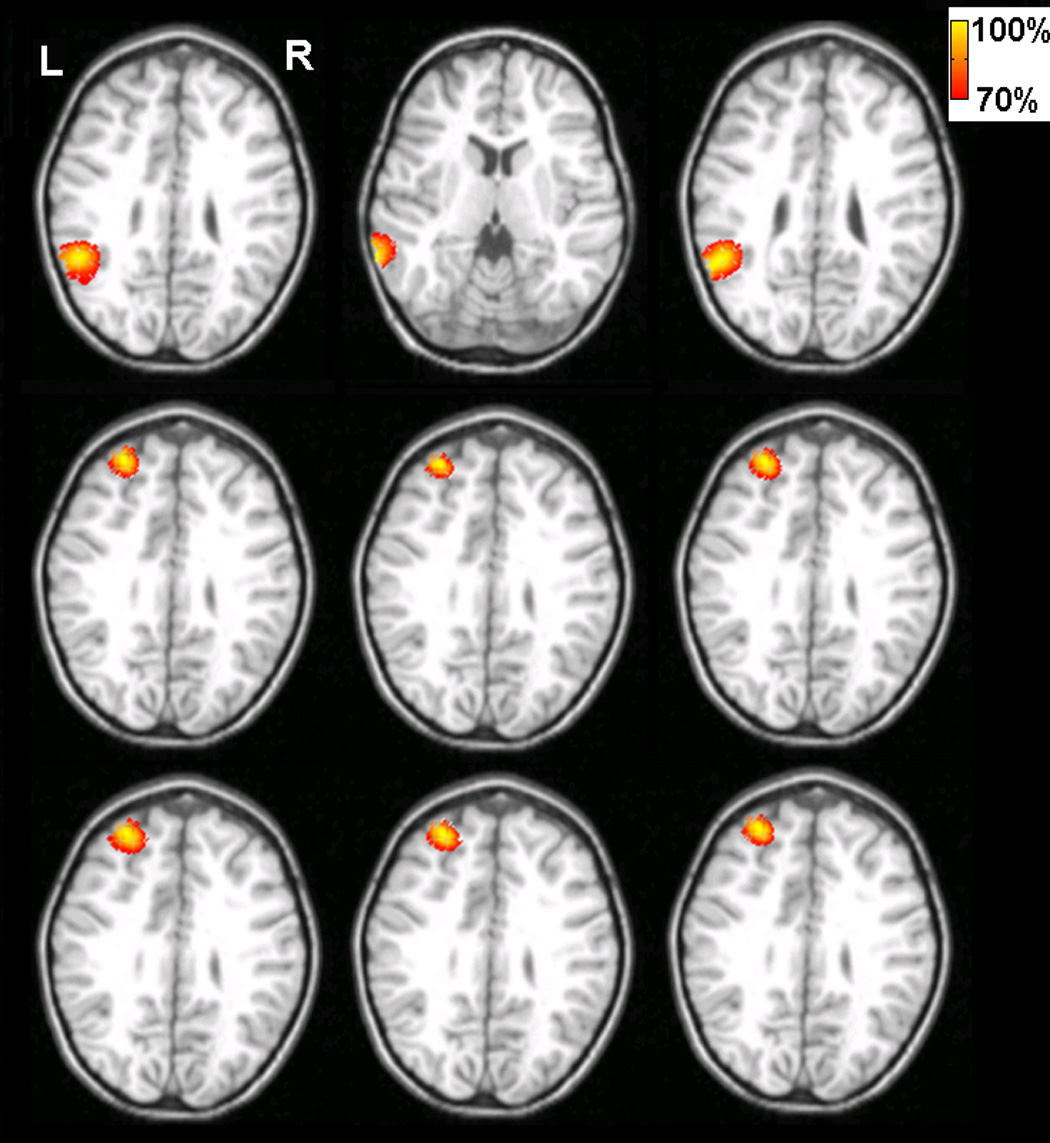
The tomography of the strengths of the current sources estimated by using the present ECoG-CDR method at the peak time of other 9 interictal spikes of the pediatric epilepsy patient. Every sub figure shows the axial view cut from the point with its maximum reconstructed current density value and the threshold is set at 70% of its maximum current density value.
IV. Discussion
In the present study, we have investigated the 3-dimensional current density distribution from the intracranial ECoG recording, using a head volume conductor model incorporating the scalp, skull, CSF, brain and implanted silastic ECoG grids, with the aid of the finite element method. The complex realistic geometry of head was derived from the MR and CT images to take into account the patient-specific geometry that may influence the accuracy of current density reconstruction. The FEM is used to construct the lead field matrix between the 3D current sources and the subdural ECoG signals. The aim of the development of the present ECoG based source reconstruction method is to provide a high resolution estimation of the 3D distribution of brain electrical sources when the subdural ECoG recordings are available. Such method may be in particular useful for deep sources which are far away from the subdural ECoG electrode grids. While we presented our results on distributed current density reconstruction, the present method is applicable to solve other brain inverse problems such as equivalent dipole localization using ECoGs, or estimation of the electric potential over the 3D brain volume.
The performance of the present FEM-based ECoG-CDR method has been evaluated by computer simulations. The localization accuracy has been investigated in detail based upon a number of single dipole source configurations and the performance of the ECoG-CDR has also been compared with that of the EEG-CDR using the scalp EEG measurements, when there is no subdural ECoG grid being implanted. According to the locations of the dipole sources in the computer simulations, the 7 dipole groups can be divided into 3 major categories, shown in Fig. 1(c). The 1st category consists of the 1st, 2nd, 3rd and 4th dipole groups, which are well covered by the implanted ECoG grids. The 1st dipole group is located exactly below the center of the parietal ECoG grid and the locations of the 2nd, 3rd and 4th groups move toward the edge of the grid with distances of 10 mm, 20 mm and 30 mm respectively from the 1st group. The 2nd category consists only of the 5th dipole group which is located under the edge of the parietal ECoG grid. The 3rd category consists of the 6th and 7th dipole groups which lie outside of the region covered by the parietal ECoG grid.
From the computer simulation results shown in Fig. 3, we can see that the present ECoG-CDR method returns high resolution results for the 1st category of dipole sources with both radial and tangential dipole moments. These are fully covered by the ECoG grid and the mean localization error of the sources with source depth of less than 40 mm are less than 10 mm except for one case (the dipole source in the 2nd dipole group with a depth of 40mm and a tangential moment). The mean localization error is less than 5 mm for the sources when the source depth is less than 30 mm in the first three dipole groups. In a total of 80 simulation cases for the 1st category (4 dipole groups × 10 dipole sources × 2 dipole directions), the present ECoG-CDR shows enhanced performance as compared with the EEG-CDR in a majority of the cases (76 out of 80). The explanation for this finding is that the intracranial ECoG have a direct access to epileptic brain activity with much less smoothing low pass filtering effects of the skin/bone layers and higher SNR, which led to enhanced performance than the extracranial scalp EEG based CDR results. This finding can also be explained that the intracranial ECoG measurement is made in the vicinity of brain electrical sources without being affected by the low-conductivity skull, which should lead to less ill-posedness in the inverse problem.
For the dipole sources in the 5th dipole group, the mean localization error curves in Fig. 3 indicate that the results of the ECoG-CDR vary according to the dipole depth when compared with the EEG-CDR results. The explanation for this phenomenon is that the silastic ECoG strip is an extremely low conductive material which substantially influences the electrical lead field in the finite element model (Zhang et al, 2006a) and accordingly introduces big variation in the current density reconstruction when the dipoles are located under the edge of the silastic ECoG pad. We used the weighted minimum-norm algorithm to balance the influence of the model’s geometric inhomogeneity on the lead field and it works well for the dipole sources fully covered by the ECoG strips as described above. However, the dipole sources located below the edges of the ECoG grid are too complicated to be handled in this manner. The EEG-CDR outperforms the ECoG-CDR for the dipole sources in the 3rd category which are outside of the region covered by the implanted ECoG grids. The reason for this is that the major activities on the cortical surface produced by the brain sources cannot be measured by the implanted ECoG grids in this case. From the comparison between the ECoG-CDR and the EEG-CDR with a single dipole source, we can see that the ECoG-CDR shows enhanced performance than the EEG-CDR for the brain sources covered by the implanted ECoG grids, but will not be suitable for imaging and localizing brain sources lying outside of the regions covered by the ECoG grids. This finding suggests that the ECoG-CDR will work well for brain sources well covered by the ECoG grids, but should not be used for potential sources out of the regions covered by the ECoG grids. In a clinical case, the planning of ECoG grid implantation in epilepsy patients is determined using clinical data: ictal features, scalp EEG and structural MRI findings (Bénar et al, 2006) in order to make sure the ECoG grids cover the major brain activities of interest. This means that most of the clinical cases fit within the 1st category in which the ECoG-CDR may play a role in imaging and localizing brain electrical sources with enhanced spatial resolution and performance.
The performance of the ECoG-CDR has been further investigated by using multiple dipole sources under a well controlled simulation protocol. There are two categories of dipole configurations used in the computer simulations: the 1st category consists of dipole pairs in which one is from the 1st dipole group and the other is from the 3rd group and the 2nd category consists of dipole pairs in which one is from the 1st dipole group and the other is from the 4th group. From the dipole configuration shown in Fig. 1 (c), we can see that the dipole pairs in the 1st category are more difficult to distinguish than the dipole pairs at the same depth in the 2nd category because the inter-source distance in the 1st category is smaller than that in the 2nd category. The present ECoG-CDR results demonstrates the ability to distinguish separate sources in the 1st category at a maximal source depth of 25 mm, but it is difficult for the EEG-CDR to distinguish separate dipole sources with a depth of 10 mm. We applied the EEG-CDR to the less challenging case, i.e. the 2nd category of dipole pairs, and it showed the ability to distinguish the separate dipole sources at a depth of less than 15 mm (note that in this case, the inter-source distance in the 2nd category of dipole pairs was almost 1.5 times larger than in the dipole pairs from the 1st category). These computer simulation results show that the ECoG-CDR provides enhanced performance in distinguishing and imaging two separate dipole sources than the EEG-CDR method.
Note that, the present EEG-CDR computer simulation results represent a comparable error range as compared with the previous 3D EEG-based current density reconstruction results using the weighted minimum norm algorithm (Pascual-Marqui et al, 1994; Ding et al, 2005). While the other studies were conducted from the scalp EEG the error range may represent the intrinsic accuracy of the weighted minimum norm solution in localizing focal sources.
An epilepsy patient has been studied using the present ECoG-CDR method and several interictal epileptiform spikes were analyzed. Fig. 8 and Fig. 9 show the 3D current density estimation results from the ECoG-CDR in an epilepsy patient using the intra-cranial electrical recordings for a frontal and parietal spike respectively. We can see that the ECoG-CDR can reconstruct the major features of the 3D current distribution produced by the brain activities. We also notice that the highest resolution results were obtained from the ECoG recordings at the peak point of the interictal spikes and the resolution decreased as the time instant moved away from the peak point. The reason for this shall be that the SNR of the recordings decrease as the measuring instant moves away from the peak point.
A major motivation for the development of ECoG based source reconstruction methods is due to the improved SNR of ECoG vs. scalp EEG and the less effect of the low conductivity skull. For the eleven interictal spikes studied in the present study, the average value of noise level from ECoG recordings was 13.3% (SNR 7.5) and the average value of noise level for the other eleven interictal spikes, which are from pre-operational EEG recordings and used as a comparison with ECoG recordings, was 23.3% (SNR 4.3). This data indicate the enhanced SNR of ECoG as compared with that of scalp EEG, and suggest the potential applications of the present approach to provide enhanced source reconstruction in patients where ECoG data are available.
Note that a previous study (Fuchs et al., 2007) reported an effort to estimate the underlying brain sources from ECoG by employing a simplified single-layer BEM model of the brain. In the study of Fuchs et al. (2007), non-insulating head tissues out of the brain were ignored to simplify the problem. In the present study detailed conductivity profiles consisting of the brain, CSF, skull, scalp and the ECoG base pads have been taken into consideration in modeling electric field with the aid of FEM (Fig. 11). Fig. 12 shows 2 examples of comparison between the cortical potential distributions due to a current dipole located in the simplified single-layer brain model (a1, a2) and in the present realistic inhomogeneous FEM head model (c1, c2). Fig. 12(a1, c1) refers to the 5th tangential dipole in the first dipole group (Fig. 1); whereas Fig. 12(a2, c2) refers to the 6th tangential dipole in the 3rd dipole group. Note differences in cortical potential distributions are observed when using different head volume conductor models, suggesting the effect of the volume conductor out of the brain tissue. In this comparison, the FEM was used in both head models (Fig. 11) in order to avoid possible numerical discrepancies introduced by different numerical techniques. The correlation coefficients (CC) between the potential distributions of the full FEM head model and the simplified single-layer brain model are lower than 94.8%, suggesting that ignoring the conductive medium surrounding the brain may have influence on the potential distributions on the ECoG grids. While the detailed comparison between the two head models on ECoG and ECoG based source imaging is beyond the scope of the present paper, Fig. 12 suggests that more accurate representation of cortical potentials can be obtained when considering the conductive medium out of the brain during clinical ECoG recording with the aid of FEM.
Fig. 11.
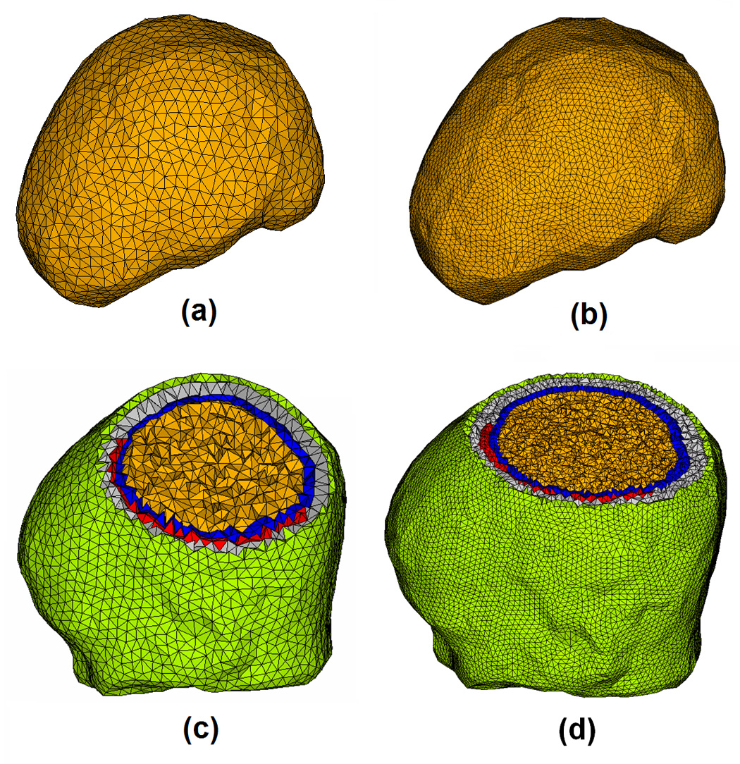
The single-layer brain model (a), high density single-layer brain model (b), full head FE model (c) and high density full head FE model (d). The full head FE model consists of the scalp (green), skull (gray), CSF (blue), brain (yellow) and silastic subdural ECoG grid (red) with 84,888 tetrahedron elements and 15,407 nodes in (c) and 620,248 tetrahedron elements and 107,719 Nodes in (d).
Fig. 12.
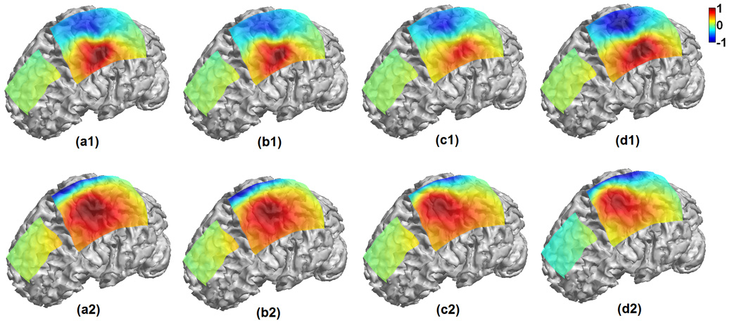
Comparison of cortical potential distributions on the ECoG grids due to dipole sources when using a single-layer brain model (a1, a2), high density single-layer brain model (b1, b2), full head FE model (c1, c2) and high resolution FE model (d1, d2). (a1, b1, c1 and d1) refers to the 5th tangential dipole in the 1st dipole group; whereas (a2, b2, c2 and d2) refers to the 6th tangential dipole in the 3rd dipole group. The correlation coefficient (CC) between (a1) and (c1) is 94.78%, CC between (a2) and (c2) is 90.13%, CC between (a1) and (b1) is 99.90%, CC between (a2) and (b2) is 99.99%, CC between (c1) and (d1) is 99.98%, and CC between (c2) and (d2) is 99.91%.
Also note that the local refine mesh generation technique was used in building the FEM model (Fig. 1) used in the present study. This technique generates the fine FEM mesh in the area consisting of more complicated geometry, for example, the area around the ECoG pad and the CSF layer, while generating the coarse FEM mesh in the area with relative simplified geometry, for example the interior of the brain. The local refine mesh generation technique helps to decrease computation load by maintaining the satisfactory calculation accuracy, which is important in implementing the research tasks with high computational loads involved like the presented ECoG-CDR using FEM. In order to address the question if the present FEM meshing is sufficient for the ECoG-CDR computation, we constructed a high density FEM model based on the same patient’s MR and CT data, and compared the results in two cases using both the FEM head model and the high density FEM head model. Fig. 11 shows the two FEM models for the brain and for the entire head with different finite elements. The potential distributions on the ECoG grids due to dipole sources using those four models are calculated via the forward solver and shown in Fig. 12. The high CC values (over 99.9%) between the simulated ECoG distributions of the regular and high-resolution full FEM head models, and the high CC values (over 99.9%) between the simulated ECoG distributions of the regular and high-resolution single-layer brain models indicate that the local refine meshing based FEM models can provide satisfactory solutions for the present ECoG-CDR research.
Fuchs et al’s study (2007) used the extended and cortically constrained source model in their current density reconstruction with the aid of a single simplified BEM brain-model. In the present study, we employed a 3D source model covering the whole brain region, which provided the source depth information in the current density reconstruction results, and investigated the influence of the source depth on the present ECoG-CDR’s capability of distinguishing and imaging multiple separate dipole sources by comparing with the EEG-CDR.
In summary, we have investigated 3-dimensional current density reconstruction to localize the brain electrical activities from the intracranial ECoG recordings with accurate head volume conductor modeling by means of the finite element method. Our ECoG-CDR method incorporates the complex finite element head model and weighted minimum norm regularization to avoid the boundary condition changes and the lead field distortions in the head volume conductor. The merits of the ECoG-CDR includes the ability to use high SNR subdural ECoG recordings to solve the brain inverse problem when such ECoG recordings are available and the anticipated brain sources are in regions covered by the ECoG grids. The present promising simulation and human results suggest that the ECoG-CDR may provide an alternative means for source localization and imaging aiding presurgical and surgical planning in epilepsy patients.
Acknowledgement
The authors would like to thank Dr. Lei Ding, Christopher Wilke, and Zhongming Liu for useful discussions. This work was supported in part by NIH RO1EB007920, RO1EB00178, NSF BES-0411898, BES-0602957, and a grant from the Institute for Engineering in Medicine at the University of Minnesota.
Reference
- Astolfi L, De Vico Fallani F, Cincotti F, Mattia D, Marciani MG, Bufalari S, Salinari S, Colosimo A, Ding L, Edgar JC, Heller W, Miller GA, He B, Babiloni F. Imaging functional brain connectivity patterns from high-resolution EEG and fMRI via graph theory. Psychophysiology. 2007a;44(6):880–893. doi: 10.1111/j.1469-8986.2007.00556.x. [DOI] [PubMed] [Google Scholar]
- Astolfi L, Cincotti F, Mattia D, Marciani MG, Baccala L, de Vico Fallani F, Salinari S, Ursino M, Zavaglia M, Ding L, Edgar JC, Miller GA, He B, Babiloni F. A comparison of different cortical connectivity estimators for high resolution EEG recordings. Human Brain Mapping. 2007b;28(2):143–157. doi: 10.1002/hbm.20263. [DOI] [PMC free article] [PubMed] [Google Scholar]
- Babiloni F, Babiloni C, Carducci F, Fattorini L, Anello C, Onorati P, Urbano A. High resolution EEG: A new model-dependent spatial deblurring method using a realistically-shaped MR-constructed subject’s head model. Electroenceph. Clin. Neurophysiol. 1997;102:69–80. doi: 10.1016/s0921-884x(96)96508-x. [DOI] [PubMed] [Google Scholar]
- Babiloni F, Babiloni C, Carducci F, Romani GL, Rossini PM, Angelone LM, Cincotti F. Multimodal integration of high-resolution EEG and functional magnetic resonance imaging data: a simulation study. Neuroimage. 2003;19:1–15. doi: 10.1016/s1053-8119(03)00052-1. [DOI] [PubMed] [Google Scholar]
- Babiloni F, Babiloni C, Carducci F, Cincotti F, Astolfi L, Basilisco A, Rossini PM, Ding L, Ni Y, Cheng J, Christine K, Sweeney J, He B. Assessing time-varying cortical functional connectivity with the multimodal integration of high resolution EEG and fMRI data by directed transfer function. NeuroImage. 2005;24:118–131. doi: 10.1016/j.neuroimage.2004.09.036. [DOI] [PubMed] [Google Scholar]
- Bénar CG, Grova C, Kobayashi E, Bagshaw AP, Aghakhani Y, Dubeau F, Gotman J. EEG-fMRI of epileptic spikes: Concordance with EEG source localization and intracranial EEG. NeuroImage. 2006;30:1161–1170. doi: 10.1016/j.neuroimage.2005.11.008. [DOI] [PubMed] [Google Scholar]
- Cuffin BN. A method for localizing EEG sources in realistic head models. IEEE Trans. Biomed. Eng. 1995;42:68–71. doi: 10.1109/10.362917. [DOI] [PubMed] [Google Scholar]
- Dale AM, Sereno MI. Improved localization of cortical activity by combining EEG and MEG with MRI cortical surface reconstruction: a linear approach. J. Cognit. Neurosci. 1993;5:162–176. doi: 10.1162/jocn.1993.5.2.162. [DOI] [PubMed] [Google Scholar]
- Ding L, Lai Y, He B. Low resolution brain electromagnetic tomography in a realistic geometry head model: a simulation study. Phys. Med. Biol. 2005;50:45–56. doi: 10.1088/0031-9155/50/1/004. [DOI] [PubMed] [Google Scholar]
- Ding L, Worrell GA, Lagerlund TD, He B. Ictal source analysis: localization and imaging of causal interactions in humans. NeuroImage. 2007;34:575–586. doi: 10.1016/j.neuroimage.2006.09.042. [DOI] [PMC free article] [PubMed] [Google Scholar]
- Ding L, He B. Sparse Source Imaging in EEG with Accurate Field Modeling. Human Brain Mapping. 2007 doi: 10.1002/hbm.20448. [DOI] [PMC free article] [PubMed] [Google Scholar]
- Engel J, Jr, Rausch R, Lieb JP, Kuhl DE, Grandall PH. Correlation of criteria used for localizing epileptic foci in patients considered for surgical therapy of epilepsy. Ann Neurol. 1981;9:215–224. doi: 10.1002/ana.410090303. [DOI] [PubMed] [Google Scholar]
- Finke S, Gulrajani RM, Gotman J. Conventional and reciprocal approaches to the inverse dipole localization problem of electroencephalography. IEEE Trans Biomed. Eng. 2003;50:657–666. doi: 10.1109/TBME.2003.812198. [DOI] [PubMed] [Google Scholar]
- Fuchs M, Wagner M, Kohler T, Wischmann HA. Linear and nonlinear current density reconstructions. J Clin Neurophysiol. 1999;16:267–295. doi: 10.1097/00004691-199905000-00006. [DOI] [PubMed] [Google Scholar]
- Fuchs M, Wagner M, Kastner JM. Development of Volume Conductor and Source Models to Localize Epileptic Foci. Journal of Clinical Neurophysiology. 2007;24(2):101–119. doi: 10.1097/WNP.0b013e318038fb3e. [DOI] [PubMed] [Google Scholar]
- Gevins A, Le J, Martin NK, Brickett P, Desmond J, Reutter B. High resolution EEG: 124-channel recording, spatial deblurring and MRI integration method. Electroenceph clin Neurophysiol. 1994;90:337–358. doi: 10.1016/0013-4694(94)90050-7. [DOI] [PubMed] [Google Scholar]
- Gulrajani RM. Bioelectricity and Biomagnetism. New York: John Wiley & Sons, Inc.; 1998. [Google Scholar]
- Grave de Peralta Menendez R, Gonzalez Andino SL, Morand S, Michel CM, Landis T. Imaging the electrical activity of the brain: ELECTRA. Hum Brain Mapp. 2000;9:1–12. doi: 10.1002/(SICI)1097-0193(2000)9:1<1::AID-HBM1>3.0.CO;2-#. [DOI] [PMC free article] [PubMed] [Google Scholar]
- Hämäläinen MS, Ilmoniemi RJ. Interpreting measured magnetic fields of the brain: estimates of current Distributions. Helsinki University of Technology; Technical Report TKK-F-A559. 1984
- Hämäläinen MS, Sarvas J. Realistic conductivity geometry model of the human head for interpretation of neuromagnetic data. IEEE Trans. Biomed. Eng. 1989;36:165–171. doi: 10.1109/10.16463. [DOI] [PubMed] [Google Scholar]
- Hämäläinen MS, Ilmoniemi RJ. Interpreting magnetic fields of the brain: minimum norm estimates. Med Biol Eng Comput. 1994;32:35–42. doi: 10.1007/BF02512476. [DOI] [PubMed] [Google Scholar]
- Hansen PC. Analysis of discrete Ill-posed problems by means of L-curve. SIAM Review. 1992;43:561–580. [Google Scholar]
- He B, Musha T, Okamoto Y, Homma S, Nakajima Y, Sato T. Electrical dipole tracing in the brain by means of the boundary element method and its accuracy. IEEE Trans. Biomed. Eng. 1987;34:406–414. doi: 10.1109/tbme.1987.326056. [DOI] [PubMed] [Google Scholar]
- He B, Wang Y, Pak S, Ling Y. Cortical source imaging from scalp electroencephalograms. Med. Biol. Eng. Comput. 1996;34:257–258. [Google Scholar]
- He B, Wang YH, Wu DS. Estimating cortical potentials from scalp EEG’s in a realistically shaped inhomogeneous head model. IEEE Trans Biomed Eng. 1999;46:1264–1268. doi: 10.1109/10.790505. [DOI] [PubMed] [Google Scholar]
- He B, Lian J, Spencer KM, Dien J, Donchin E. A cortical potential imaging analysis of the P300 and novelty P3 components. Hum. Brain Mapp. 2001;12:120–130. doi: 10.1002/1097-0193(200102)12:2<120::AID-HBM1009>3.0.CO;2-V. [DOI] [PMC free article] [PubMed] [Google Scholar]
- He B, Yao D, Lian J, Wu DS. An equivalent current source model and Laplacian weighted minimum norm current estimates of brain electrical activity. IEEE Trans. Biomed. Eng. 2002a;49:277–288. doi: 10.1109/10.991155. [DOI] [PubMed] [Google Scholar]
- He B, Yao D, Lian J. High resolution EEG: on the cortical equivalent dipole layer imaging. Clin.Neurophysiol. 2002b;113:227–235. doi: 10.1016/s1388-2457(01)00740-4. [DOI] [PubMed] [Google Scholar]
- He B, Zhang X, Lian J, Sasaki H, Wu DS, Towle VL. Boundary element method-based cortical potential imaging of somatosensory evoked potentials using subjects’ magnetic resonance images. Neuroimage. 2002c;16:564–576. doi: 10.1006/nimg.2002.1127. [DOI] [PubMed] [Google Scholar]
- He B, Lian J. Spatio-temporal functional neuroimaging of brain electric activity. Crit. Rev. Biomed. Eng. 2002;30:283–306. doi: 10.1615/critrevbiomedeng.v30.i456.30. [DOI] [PubMed] [Google Scholar]
- He B, Lian J. Electrophysiological Neuroimaging. In: He B, editor. Neural Engineering. Kluwer Academic/Plenum Publishers; 2005. pp. 221–262. [Google Scholar]
- Korzyukov O, Pflieger ME, Wagner M, Bowyer SM, Rosburg T, Sundaresan K, Elger CE, Boutros NN. Generators of the intracranial P50 response in auditory sensory gating. NeuroImage. 2007;35:814–826. doi: 10.1016/j.neuroimage.2006.12.011. [DOI] [PMC free article] [PubMed] [Google Scholar]
- Leahy RM, Mosher JC, Spencer ME, Huang MX, Lewine JD. A study of dipole localization accuracy for MEG and EEG using a human skull phantom. Electroencephalogr Clin Neurophysiol. 1998;107:159–173. doi: 10.1016/s0013-4694(98)00057-1. [DOI] [PubMed] [Google Scholar]
- Liu ZM, Kecman F, He B. Effects of fMRI-EEG mismatches in cortical current density estimation integrating fMRI and EEG: a simulation study. Clinical Neurophysiology. 2006;117:1610–1622. doi: 10.1016/j.clinph.2006.03.031. [DOI] [PMC free article] [PubMed] [Google Scholar]
- Liu ZM, He B. FMRI-EEG Integrated Cortical Source Imaging by use of Time-Variant Spatial Constraints. NeuroImage. 2008;39(3):1198–1214. doi: 10.1016/j.neuroimage.2007.10.003. [DOI] [PMC free article] [PubMed] [Google Scholar]
- Merlet I, Gotman J. Dipole modeling of scalp electroencephalogram epileptic discharges: correlation with intracerebral fields Clin. Neurophysiol. 2001;112:414–430. doi: 10.1016/s1388-2457(01)00458-8. [DOI] [PubMed] [Google Scholar]
- Mosher JC, Lewis PS, Leahy RM. Multiple dipole modeling and localization from spatiotemporal MEG data. IEEE Trans. Biomed. Eng. 1992;39:541–557. doi: 10.1109/10.141192. [DOI] [PubMed] [Google Scholar]
- Mosher JC, Leahy RM, Lewis PS. EEG and MEG: forward solutions for inverse methods. IEEE Trans. Biomed. Eng. 1999;46:245–259. doi: 10.1109/10.748978. [DOI] [PubMed] [Google Scholar]
- Nunez P, Silibertein RB, Cdush PJ, Wijesinghe RS, Westdrop AF, Srinivasan R. A theoretical and experimental study of high resolution EEG based on surface Laplacian and cortical imaging. Electroenceph clin Neurophysiol. 1994;90:40–57. doi: 10.1016/0013-4694(94)90112-0. [DOI] [PubMed] [Google Scholar]
- Pascual-Marqui RD, Michel CM, Lehmann D. Low resolution electromagnetic tomography: a new method for localizing electrical activity in the brain. Int. J. Psychophysiol. 1994;18:49–65. doi: 10.1016/0167-8760(84)90014-x. [DOI] [PubMed] [Google Scholar]
- Pascual-Marqui RD. In: Reply to comments by Hämäläinen, Ilmoniemi and Nunez Source Localization: Continuing Discussion of the Inverse Problem. Skrandies W, editor. 1995. Newsletter No. 6 (ISSN 0947-5133) [Google Scholar]
- Pascual-Marqui RD. Review of methods for solving the EEG inverse problem. Int. J. Bioelectromagnetism. 1999;1:75–86. [Google Scholar]
- Phillips JW, Leahy RM, Mosher JC. MEG-based imaging of focal neuronal current sources. IEEE Trans. Med. Imaging. 1997;13:338–348. doi: 10.1109/42.585768. [DOI] [PubMed] [Google Scholar]
- Rush S, Driscoll DA. EEG electrode sensitivity-An application of reciprocity. IEEE Trans Biomed. Eng. 1969;16:15–22. doi: 10.1109/tbme.1969.4502598. [DOI] [PubMed] [Google Scholar]
- Scherg M, Von Cramon D. Two bilateral sources of the AEP as identified by a spatio-temporal dipole model. Electroenceph. Clin. Neurophysiol. 1985;62:32–44. doi: 10.1016/0168-5597(85)90033-4. [DOI] [PubMed] [Google Scholar]
- Silvester PP, Ferrari RL. Finite elements for electrical engineering. New York: Cambridge University Press; 1996. [Google Scholar]
- Towle VL, Khorasani L, Uftring S, Pelizzari C, Erickson RK, Spire JP, Hoffmann K, Chu D, Scherg M. Noninvasive identification of human central sulcus: a comparison of gyral morphology, functional MRI, dipole localization, and direct cortical mapping. NeuroImage. 2003;19:684–697. doi: 10.1016/s1053-8119(03)00147-2. [DOI] [PubMed] [Google Scholar]
- Wang Y, He B. A computer simulation study of cortical imaging from scalp potentials. IEEE Trans. Biomed. Eng. 1998;45:724–735. doi: 10.1109/10.678607. [DOI] [PubMed] [Google Scholar]
- Xu XL, Xu B, He B. An alternative subspace approach to EEG dipole source localization. Phys. Med. Biol. 2004;49:327–343. doi: 10.1088/0031-9155/49/2/010. [DOI] [PubMed] [Google Scholar]
- Zhang YC, Zhu SA, He B. A Second-Order Finite Element Algorithm for Solving the Three-Dimensional EEG Forward Problem. Phys. Med. Biol. 2004;49:2975–2987. doi: 10.1088/0031-9155/49/13/014. [DOI] [PubMed] [Google Scholar]
- Zhang YC, Ding L, van Drongelen W, Hecox K, Frim DM, He B. A cortical potential imaging study from simultaneous extra- and intracranial electrical recordings by means of the finite element method. NeuroImage. 2006a;31:1513–1524. doi: 10.1016/j.neuroimage.2006.02.027. [DOI] [PMC free article] [PubMed] [Google Scholar]
- Zhang YC, van Drongelen W, He B. Estimation of in vivo brain-to-skull conductivity ratio in humans. Applied Physics Letter. 2006b;89:2239031–2239033. doi: 10.1063/1.2398883. [DOI] [PMC free article] [PubMed] [Google Scholar]