Principles of Flexible Protein-Protein Docking

Abstract

Treating flexibility in molecular docking is a major challenge in cell biology research. Here we describe the background and the principles of existing flexible protein-protein docking methods, focusing on the algorithms and their rational. We describe how protein flexibility is treated in different stages of the docking process: in the preprocessing stage, rigid and flexible parts are identified and their possible conformations are modeled. This preprocessing provides information for the subsequent docking and refinement stages. In the docking stage, an ensemble of pre-generated conformations or the identified rigid domains may be docked separately. In the refinement stage, small-scale movements of the backbone and side-chains are modeled and the binding orientation is improved by rigid-body adjustments. For clarity of presentation, we divide the different methods into categories. This should allow the reader to focus on the most suitable method for a particular docking problem.

Introduction

Most cellular processes are carried out by protein-protein interactions. Predicting the three-dimensional structures of protein-protein complexes (docking) can shed light on their functional mechanisms and roles in the cell. Understanding and modeling the bound configuration are major scientific challenges. The structures of the complexes provide information regarding the interfaces of the proteins and assist in drug design. Docking can assist in predicting protein-protein interactions, in understanding signaling pathways and in evaluating the affinity of complexes.

Upon binding, proteins undergo conformational changes that include both backbone and side-chain movements¹. Backbone flexibility can be divided into two major types: large-scale domain motions, such as “shear” and “hinge-bending” motion (Figure 1 (a-d)), and disordered regions such as flexible loops (Figure 1 (e)). The first docking methods treated proteins as rigid bodies in order to reduce the search space for optimal structures of the complexes^{2, 3}. However, ignoring flexibility could prevent docking algorithms from recovering native associations. Accounting for flexibility is also essential for the accuracy of the solutions. In addition, flexibility must also be taken into account if the docked structures were determined by homology modeling⁴ or if loop conformations were modeled⁵.

Figure 1.

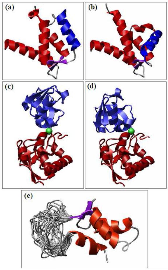
Protein flexibility types. (a,b) Shear motion, demonstrated in two conformations of S100 Calcium sensor (PDB-id: 1K9P, 1K9K). The blue helix “slides” on the rest of the protein. (c,d) Hinge motion, demonstrated in two conformations of LAO binding protein (PDB-id: 1LAO, 1LAF). The hinge location is shown as a green sphere. (e) Flexible loop in the ribosomal protein L1 (PDB-id: 1FOX). The different conformations of the loop were determined experimentally by NMR.

Incorporating flexibility in a docking algorithm is much more difficult than performing rigid-body docking. The high number of degrees of freedom not only significantly increases the running time, but also results in a higher rate of false-positive solutions. These must be scored correctly in order to identify near-native results⁶. Consequently, existing docking methods limit the flexibility to certain types of motions. In addition, many of these methods allow only one of the proteins in the complex to be flexible.

The general scheme of flexible docking can be divided into four major stages as depicted in Figure 2. The first is a preprocessing stage. In this stage the proteins are analyzed in order to define their conformational space. An ensemble of discrete conformations can be generated from this space and used in further cross-docking, where each protein conformation is docked separately. This process simulates the conformational selection model^{7, 8}. The analysis can also identify possible hinge locations. In this case the proteins can be divided into their rigid parts and be docked separately. The second is a rigid-docking stage. The docking procedure aims to generate a set of solution candidates with at least one near-native structure. The rigid docking should allow some steric clashes because proteins in their unbound conformation can collide when placed in their native interacting position. The next stage, called refinement, models an induced fit⁹. In this stage each candidate is optimized by small backbone and side-chain movements and by rigid-body adjustments. It is difficult to simultaneously optimize the side-chain conformations, the backbone structure and the rigid-body orientation. Therefore, the three can be optimized in three separately repeated successive steps. The resulting refined structures have better binding energy and hardly include steric clashes. The final stage is scoring. In this stage the candidate solutions are scored and ranked according to different parameters such as binding energy, agreement with known binding sites, deformation energy of the flexible proteins, and existence of energy funnels^{10, 11}. The goal of this important stage is to identify the near-native solutions among the candidates. In this review we do not address the scoring function problem. A detailed review of scoring schemes was published by Halperin et al.³.

Figure 2.

A general scheme of flexible docking procedure. (a) Protein flexibility analysis methods are described in section 2. (b) Rigid docking with soft interface, ensemble docking of different conformations and backbone refinement methods are described in section 3. (c) Side-chain refinement methods are described in section 4. (d) Rigid body optimization methods are mentioned in the discussion.

Two flexible docking reviews were published recently^{12, 13}. These articles present a variety of docking methods that incorporate protein flexibility. However, we believe that a more detailed and comprehensive review would be useful for the docking community. Our review provides a description of the computational algorithms behind the docking methods. The division into categories used in this article can help the reader choose the most suitable method for a particular docking problem.

Our review includes three major parts, corresponding to different flexible docking procedures. The first part describes protein flexibility analysis methods. The second part discusses the treatment of backbone flexibility in current docking algorithms. The third, side-chain refinement part reviews methods for prediction of bound side-chain conformations. Finally, existing methods that handle both backbone and side-chain flexibility are described.

2 Protein Flexibility Analysis

Protein flexibility analysis methods, reviewed below, can be classified into three major categories:

• 1Methods for generating an ensemble of discrete conformations. Ensembles of conformations are widely used in cross-docking and in the refinement stage of the docking procedure. The different conformations can be created by analyzing different experimentally solved protein structures or by using Molecular Dynamics (MD) simulation snapshots.
• 2Methods for determining a continuous protein conformational space. The conformational space can be used as a continuous search space for refinement algorithms. In addition, many flexible docking methods sample this pre-calculated conformational space in order to generate a set of discrete conformations This group of methods includes Normal Modes Analysis (NMA) and Essential Dynamics.
• 3Methods for identifying rigid and flexible regions in the protein. These methods include the rigidity theory and hinge detection algorithms.

2.1 Conformational Ensemble Analysis

Using different solved 3D structures (by X-ray and NMR) of diverse conformations of the same protein, or of homologous proteins, is probably the most convenient way to obtain information relating to protein flexibility. Using such conformers, one can generate new viable conformations which might exist during the transition between one given conformation to another. These new conformations can be generated by “morphing” techniques^{14, 15} which implement linear interpolations, but have limited biological relevance.

Known structures of homologs or of different conformations of the same protein can also be useful in detecting rigid domains and hinge locations. Boutonnet et al.¹⁶ developed one of the first methods for an automated detection of hinge and shear motions in proteins. The method uses two conformations of the same protein. It identifies structurally similar segments and aligns them. Then, the local alignments are hierarchically clustered to generate a global alignment and a clustering tree. Finally the tree is analyzed to identify the hinge and shear motions. The DynDom method¹⁷ uses a similar clustering approach for identifying hinge points using two protein conformations. Given the set of atom displacement vectors, the rotation vectors are calculated for each short backbone segment. A rotation vector can be represented as a rotation point in a 3D space. A domain that moves as a rigid-body will produce a cluster of rotation points. The method uses the K-means clustering algorithm to determine the clusters and detect the domains. Finally, the hinge axis is calculated and the residues involved in the inter-domain bending are identified.

The HingeFind¹⁸ method can also analyze structures of homolog proteins in different conformations and detects rigid domains, whose superimposition achieves RMSD of less than a given threshold. It requires sequence alignment of two given protein structures. The procedure starts with each pair of aligned C_α atoms and iteratively tries to extend them by adding adjacent C_α atoms as long as the RMSD criterion holds. After all the rigid domains are identified, the rotation axes between them are calculated. Verbitsky et al.¹⁹ used the geometric hashing approach to align two molecules, and detect hinge-bent motifs. The method can match the motifs independently of the order of the amino acids in the chain. The more advanced FlexProt method^{20, 21} searches for 3D congruent rigid fragment pairs in structures of homolog proteins, by aligning every C_α pair and trying to extend the 3D alignment, in a way similar to HingeFind. Next, an efficient graph-theory method is used for the connection of the rigid parts and the construction of the full solution with the largest correspondence list, which is sequence-order dependent. The construction simultaneously detects the locations of the hinges.

2.2 Molecular Dynamics

Depending on the time scales and the barrier heights, molecular dynamics simulations can provide insight into protein flexibility. Molecular dynamics (MD) simulations are based on a force field that describes the forces created by chemical interactions²². Throughout the simulation, the motions of all atoms are modeled by repeatedly calculating the forces on each atom, solving Newton's equation and moving the atoms accordingly. Di Nola et al. ^{23, 24} were first to incorporate explicit solvent molecules into MD simulations while docking two flexible molecules. Pak et al.²⁵ applied MD using Tsallis effective potential²⁶ for the flexible docking of few complexes.

Molecular Dynamics simulations require long computational time scales and therefore are limited in the motion amplitudes. For this reason they can be used for modeling only relatively small-scale movements, which take place in nanosecond time scales, while conformational changes of proteins often occur over a relatively long period of time (∼ 1 ms)^{27, 28}. One way to speed up the simulations is by restricting the degrees of freedom to the torsional space, which allows larger integration time steps²⁹. Another difficulty is that the existence of energy barriers may trap the MD simulation in certain conformations of a protein. This problem can be overcome by using simulated annealing³⁰ and scaling methods³¹ during the simulation. For example, simulated annealing MD is used in the refinement stage of HADDOCK^{32, 33} in order to refine the conformations of both the side-chains and the backbone. Riemann et al. applied potential scaling during during MD simulations to predict side chain conformations³⁴.

In order to sample a wide conformational space and search for conformations at local minima in the energy landscape, biased methods, which were previously reviewed³⁵, can be used. The flooding technique³⁶, which is used in the GROMACS method³⁷, fills the “well” of the initial conformation in the energy landscape with a Gaussian shape “flooding” potential. Another similar method, called puddle-jumping³⁸, fills this well up to a flat energy level. These methods accelerate the transition across energy barriers and permit scanning other stable conformations.

2.3 Normal Modes

Normal Modes Analysis (NMA) is a method for calculating a set of basis vectors (normal modes) which describes the flexibility of the analyzed protein^{39, 40, 41}. The length of each vector is 3 N, where N is the number of atoms or amino acids in the protein, depending on the resolution of the analysis. Each vector represents a certain movement of the protein such that any conformational change can be expressed as a linear combination of the normal modes. The coefficient of a normal mode represents its amplitude.

A common model used for normal modes calculation is the Anisotropic Network Model (ANM), which was previously described in detail^{40, 42}. This is a simplified spring model which relies primarily on the geometry and mass distribution of a protein (Figure 3). Every two atoms (or residues) within a distance below a threshold are connected by a spring (usually all springs have a single force constant). The model treats the initial conformation as the equilibrium conformation.

Figure 3.

An example of a simplified spring model generated from a short polypeptide chain by connecting every pair of C_α atoms within a distance threshold by a spring. (a) The polypeptide chain. (b) The spring model. The normal modes calculated from this spring model describe its possible movements around the equilibrium conformation. Normal modes were shown to correlate with experimentally observed conformational changes of proteins.

The normal modes describe continuous motions of the flexible protein around a single equilibrium conformation. Theoretically, this model does not apply to proteins which have several conformational states with local free-energy minima. However, in practice, normal modes suit very well conformational changes observed between bound and unbound protein structures⁴³. Another advantage of the normal modes analysis is that it can discriminate between low and high frequency modes. The low frequency modes usually describe the large scale motions of the protein. It has been shown^{44, 43} that the first few normal modes, with the lowest frequencies, can describe much of a conformational change. This allows reducing the degrees of freedom considerably while preserving the information about the main characteristics of the protein motion. Therefore many studies^{45, 46, 47} use a subset of the lowest frequency modes for analyzing the flexibility of proteins. The normal modes can further be used for predicting hinge-bending movements⁴⁸, for generating an ensemble of discrete conformations⁴⁹ and for estimating the protein's deformation energy resulting from a conformational change^{50, 51}.

Tama and Sanejouand⁴⁴ showed that normal modes obtained from the open form of a protein correlate better with its known conformational changes, than the ones obtained from its closed form. In a recent work, Petrone and Pande⁴³ showed that the first 20 modes can improve the RMSD to the bound conformation by only up to 50%. The suggested reason was that while the unbound conformation moves mostly according to low frequency modes, the binding process activates movements related to modes with higher frequencies.

The binding site of proteins often contains loops which undergo relatively small conformational changes triggered by an interaction. This phenomenon is common in protein kinase binding pockets. Loop movements can only be characterized by high-frequency normal modes. Therefore, we would like to identify the modes which influence these loops the most, in order to focus on these in the docking process. For this reason, Cavasotto et al.⁵² have introduced a method for measuring the relevance of a mode to a certain loop. This measure of relevance favors modes which bend the loop at its edges, and significantly moves the center of the loop. It excludes modes which distort the loop or move the loop together with its surroundings. This measure was used to isolate the normal modes which are relevant to loops within the binding sites of two cAMP-dependent protein kinases (cAPKs). For each loop less than 10 normal modes were found to be relevant, and they all had relatively high frequencies. These modes were used for generating alternative conformations of these proteins, which were later used for docking. The method succeeded in docking two small ligands which could not be docked to the unbound conformations of the cAPKs due to steric clashes.

Since NMA is based on an approximation of a potential energy in a specific starting conformation, its accuracy deteriorates when modeling large conformational changes. Therefore in some studies, the normal modes were recomputed after each small displacement^{53, 54, 55}. This is an accurate but time-consuming method. Kirillova et al.⁵⁶ have recently developed an NMA-guided RRT method for exploring the conformational space spanned by 10-30 low frequency normal modes. This efficient method require a relatively small number of normal modes calculations to compute large conformational changes.

The Gaussian Network Model (GNM) is another simplified version of normal modes analysis^{57, 58} The GNM analysis uses the topology of the spring network for calculating the amplitudes of the normal modes and the correlations between the fluctuations of each pair of residues. However, the direction of each fluctuation cannot be found by GNM. This analysis is more efficient both in CPU time and in memory than the ANM analysis and therefore it can be applied on larger systems. The drawback is that the GNM calculates relatively partial information on the protein flexibility.

The HingeProt algorithm⁴⁸ analyzes a single conformation of a protein using GNM, and predicts the location of hinges and rigid parts. Using the two slowest modes, it calculates the correlation between the fluctuations of each pair of residues, i.e. their tendency to move in the same direction. A change in the sign of the correlation value between two consecutive regions in the protein suggests a flexible joint that connects rigid units.

2.4 Essential Dynamics

The Essential Dynamics approach aims at capturing the main flexible degrees of freedom of a protein, given a set of its feasible conformations⁵⁹. These degrees of freedom are described by vectors which are often called essential modes, or principal components (PC). The conformation set is used to construct a square covariance matrix (3N × 3N, where N is the number of atoms) of the deviation of each atom coordinates from its unbound position or, alternatively, average position. This matrix is then diagonalized and its eigenvectors and eigenvalues are found. These eigenvectors represent the principal components of the protein flexibility. The bigger the eigenvalues, the larger the amplitude of the fluctuation described by its eigenvector.

Mustard and Ritchie⁶⁰ used this essential dynamics approach to generate realistic starting structures for docking, which are called eigenstructures. The covariance matrix was created according to a large number of conformations, generated using the CONCOORD program⁶¹, which randomly generates 3D protein conformations that fulfill distance constraints. The eigenvectors were calculated and it has been shown⁶⁰ that the first few of these (with the largest eigenvalues) can account for many of the backbone conformational changes that occurred upon binding in seven different CAPRI targets from rounds 3-5⁶². Linear combinations of the first eight eigenvectors were later used to generate eigenstructures from each original unbound structure of these CAPRI targets. An experiment that used these eigenstructures in rigid docking showed improvements in the results compared to using the unbound structure or a model-built structure⁶⁰. An ensemble of conformations can be generated in a similar way by the Dynamite software⁶³, which also applies the essential dynamics approach on a set of conformations generated by CONCOORD.

Principle component analysis (PCA) can also be based on molecular dynamics simulations. Unlike normal mode analysis, this PCA includes the effect of the surrounding water on the flexibility. However, the results of the analysis strongly depend on the simulation's length and convergence. It has been shown that most of the conformational fluctuations observed by MD simulations⁵⁹ and some known conformational changes between unbound and bound forms⁶⁴, can be described with only few PCs.

2.5 Rigidity Theory

Jacobs et al.⁶⁵ developed a graph-theory method which analyzes protein flexibility and identifies rigid and flexible substructures. In this method a network is constructed according to distance and angle constraints, which are derived from covalent bonds, hydrogen bonds and salt bridges within a single conformation of a protein. The vertices of the network represent the atoms and the edges represent the constraints. The analysis of the network resembles a pebble game. At the beginning of the algorithm, each atom (vertex) receives three pebbles which represent three degrees of freedom (translation in 3D). The edges are added one by one and each edge consumes one pebble from one of its vertices, if possible. It is possible to rearrange the pebbles on the graph as long as the following rules hold: (1) Each vertex is always associated with exactly three pebbles which can be consumed by some of its adjacent edges. (2) Once an edge consumes a pebble it must continue holding a pebble from one of its vertices throughout the rest of the algorithm. At the end of the algorithm the remaining pebbles can still be rearranged but the specified rules divide the protein into areas in such a way that the pebbles can not move from one area to another.

The number of remaining degrees of freedom in a certain area of the protein quantifies its flexibility. For example, a rigid area will not possess more than 6 degrees of freedom (which represent translation and rotation in 3D). The algorithm can also identify hinge points, and rigid domains which are stable upon removal of constraints like hydrogen-bonds and salt bridges. This pebbles-game algorithm is implemented in a software called FIRST (Floppy Inclusion and Rigid Substructure Topography) which analyzes protein flexibility in only a few seconds of CPU time. The algorithm was tested on HIV protease, dihydrofolate reductase and adenylate kinase and was able to predict most of their functionally important flexible regions, which were known beforehand by X-ray and NMR experiments.

3 Handling Backbone Flexibility in Docking Methods

Treating backbone flexibility in docking methods is still a major challenge. The backbone flexibility adds a huge number of degrees of freedom to the search space and therefore makes the docking problem much more difficult. The docking methods can be divided into four groups according to their treatment of backbone flexibility. The first group uses soft interface during the docking and allows some steric clashes in the resulting complex models. The second performs an ensemble docking, which uses feasible conformations of the proteins, generated beforehand. The third group deals with hinge bending motions, and the last group heuristically searches for energetically favored conformations in a wide conformational search space.

3.1 Soft Interface

Docking methods that use soft interface actually perform relatively fast rigid-body docking which allows a certain amount of steric clashes (penetration). These methods can be divided into three major groups: (i) brute force techniques^{66, 67, 68} that can be significantly speeded up by FFT^{69, 70, 71, 72, 73, 74}, (ii) randomized methods^{75, 10} and (iii) shape complementarity methods^{76, 77, 78, 79, 80}. This approach can only deal with side chain flexibility and small scale backbone movements. It is assumed that the proteins are capable of performing the required conformational changes which avoid the penetrations, although the actual changes are not modeled explicitly. Since the results of this soft docking usually contain steric clashes, a further refinement stage must be used in order to resolve them.

3.2 Ensemble Docking

In order to avoid the search through the entire flexible conformational space of two proteins during the docking or refinement process, the ensemble docking approach samples an ensemble of different feasible conformations prior to docking. Next, docking of the whole ensemble is performed. The different conformations can be docked one by one (cross-docking), which significantly increases the computational time, or all together using different algorithms such as the mean-field approach presented below.

The ensemble may include different crystal structures and NMR conformers of the protein. Other structures can be calculated using computational sampling methods which are derived from the protein flexibility analysis (molecular dynamics, normal modes, essential dynamics, loop modeling, etc). Feasible structures can also be sampled using random-search methods such as Monte-Carlo and genetic algorithms.

The search for an optimal loop conformation can be performed during the docking procedure by the mean-field approach. In this method, a set of loop conformations is sampled in advance and each conformation is initialized by an equal weight. Throughout the docking, in each iteration, the weights of the conformations (copies) change according to the Boltzmann criterion, in a way that a conformation receives a higher weight if it achieves a lower free energy. The partner and the rest of the protein which interact with the loop “feel” the weighted average of the energies of their interactions with each conformation in the set. The algorithm usually converges to a single conformation for each loop, with a high weight⁸¹.

Bastard et al.⁸¹ used the mean-field approach in their MC2 method which is based on multiple copy representation of loops and Monte Carlo (MC) conformational search. Viable loop conformations were created using a combinatorial approach, which randomly selected common torsional angles for the loop backbone. In each MC step the side-chains dihedral angles and the rotation and translation variables are randomly chosen. Then, the weight of each loop is adjusted according to its Boltzmann probability. The performance of the MC2 algorithm was evaluated⁸¹ on the solved protein-DNA complex of a Drosophila Prd-paired-domain protein, which interacts with its target DNA segment by a loop of seven residues⁸². 23% of the MC2 simulations produced results in which the RMSD was lower than 1.5Å and included the selection of a loop conformation which was extremely similar to the native one. Furthermore, these results got much better energy scores than the other 77%, therefore they could be easily identified.

In a later work⁸³, the mean-field approach was introduced in the ATTRACT software and was tested on a set of eight protein-protein complexes in which the receptor undergoes a large conformational change upon binding or its solved unbound structure has a missing loop at its interaction site. The results showed that the algorithm improved the docking significantly compared to rigid docking methods.

3.3 Modeling Hinge Motion

Hinge-bending motions are common during complex creation. Hinges are flexible segments which separate relatively rigid parts of the proteins, such as domains or subdomains.

Sandak et al.^{84, 85} introduced a method which deals with this type of flexibility. The algorithm allows multiple hinge locations, which are given by the user. Hinges can be given for only one of the interacting proteins (e.g. the ligand). The algorithm docks all the rigid parts of the flexible ligand simultaneously, using the geometric hashing approach.

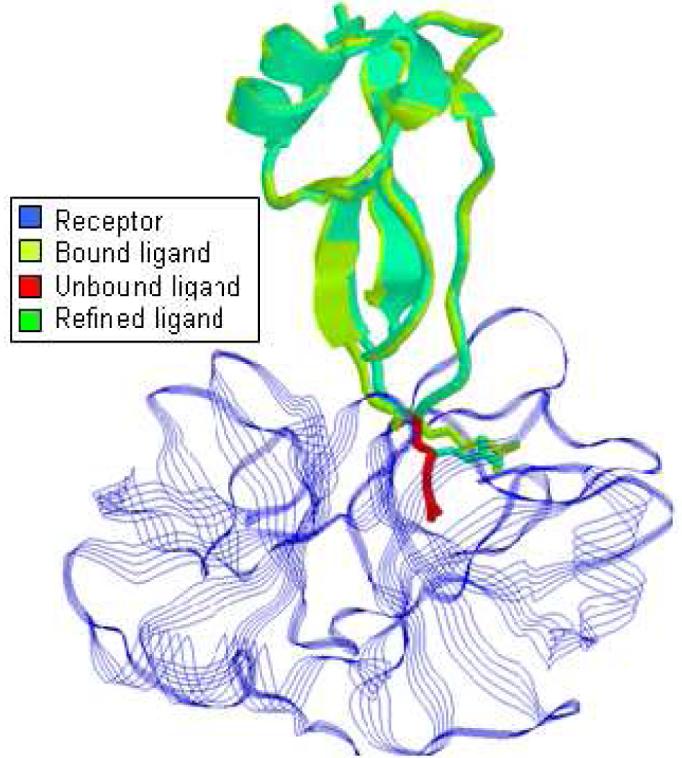
The FlexDock algorithm^{86, 87} is a more advanced method for docking with hinge-bending flexibility in one of the interacting proteins. The locations of the hinges are automatically detected by the HingeProt algorithm. The number of hinges is not limited and does not affect the running time complexity. However, the hinges must impose a chain-type topology, i.e. the subdomains separated by the hinges must form a linear chain. The algorithm divides the flexible protein into subdomains at its hinge points. These subdomains are docked separately to the second protein by the PatchDock algorithm⁷⁷. Then, an assembly graph is constructed. Each node in the graph represents a result of a subdomain rigid docking (a transformation), and the node is assigned a weight according to the docking score. Edges are added between nodes which represent consistent solutions of consecutive rigid subdomains. An edge weight corresponds to the shape complementarity score between the two subdomains represented by its two nodes. Finally, the docking results of the different subdomains are assembled to create full consistent results for the complex using an efficient dynamic programming algorithm that finds high scoring paths in the graph. This approach can cope with very large conformational changes. Among its achievements, it has predicted the bound conformation of calmodulin to a target peptide, the complex of Replication Protein A with a single stranded DNA as shown inFigure 4, and has created the only acceptable solution for the LicT dimer at the CAPRI challenge (Target 9)⁸⁶.

Figure 4.

(a) The unbound conformation of Replication Protein A in red and blue (PDB-id: 1FGU) and its target DNA strand in green. The figure shows the unbound conformation of the protein after superimposing it on its bound conformation in the solved complex structure (The superpostion was performed for visualization purpose only). (b) The bound conformation of Replication Protein A in red and blue (PDB-id: 1JMC) and the predicted bound conformation by FlexDock⁸⁶ in cyan.

Ben-Zeev et al.⁸⁸ have coped with the CAPRI challenges which included domain movements (Target 9, 11 and 13) by a rigid body multi-stage docking procedure. Each of the proteins was partitioned into its domains. Then, the domains of the two proteins were docked to each other in all possible order of steps. In each step, the current domain was docked to the best results from the previous docking step.

This multistage method requires that the native position of a subdomain will be ranked high enough in each step. This restriction is avoided in the FlexDock algorithm which in the assembling stage uses a large number of docking results for each subdomain. Therefore a full docking result can be found and be highly ranked even if its partial subdomain docking results were poorly ranked.

3.4 Refinement and Minimization Methods for Treating Backbone Flexibility

Fitzjohn and Bates⁸⁹ used a guided docking method, which includes a fully flexible refinement stage. In the refinement stage CHARMM22 all-atom force field was used to move the individual atoms of the receptor and the ligand. In addition, the forces acting on each atom were summed and converted into a force on the center-of-mass of each molecule.

Lindahl and Delarue introduced a new refinement method⁹⁰ for docking solutions which minimizes the interaction energy in a complex along 5-10 of the lowest frequency normal modes' directions. The degrees of freedom in the search space are the amplitudes of the normal modes, and a quasi-Newtonian algorithm is used for the energy minimization. The method was tested on protein-ligand and protein-DNA complexes and was able to reduce the RMSD between the docking model and the true complex by 0.3-3.6Å.

In a recent work, May and Zacharias⁵¹ accounted for global conformational changes during a systematic docking procedure. The docking starts by generating many thousands of rigid starting positions of the ligand around the receptor. Then, a minimization procedure is performed on the six rigid degrees of freedom and on five additional degrees of freedom which account for the coefficients of the five, pre-calculated, slowest frequency normal modes. The energy function includes a penalty term that prevents large scale deformations. Applying the method to several test cases showed that it can significantly improve the accuracy and the ranking of the results. However the side-chain conformations must be refined as well. The method was recently incorporated into the ATTRACT docking software.

A new data structure called Flexibility Tree (FT) was recently presented by Zhao et al.⁹¹. The FT is a hierarchical data structure which represents conformational subspaces of proteins and full flexibility of small ligands. The hierarchical structure of this data structure enables focusing solely on the motions which are relevant to a protein binding site. The representation of protein flexibility by FT combines a variety of motions such as hinge bending, flexible side-chain conformations and loop deformations which can be represented by normal modes or essential dynamics. The FT parameterizes the flexibility subspace by a relatively small number of variables. The values of these variables can be searched, in order to find the minimal energy solution. The FLIPDock⁹² method uses two FT data structures, representing the flexibility of both the ligand and the receptor. The right conformations are then searched using a genetic algorithm and a divide and conquer approach, during the docking process.

Many docking methods use Monte-Carlo methods in the final minimization step. For example, Monte-Carlo minimization (MCM) is used in the refinement stage of RosettaDock^{93, 94}. Each MCM iteration consists of three steps: (1) random rigid-body movements and backbone perturbation, in certain peptide segments which were chosen to be flexible according to a flexibility analysis performed beforehand; (2) rotamer-based side-chain refinement; (3) quasi-Newton energy minimization for relatively small changes in the backbone and side-chain torsional angles, and for minor rigid-body optimization.

Some docking methods⁹³ simply ignore flexible loops during the docking and rebuild them afterwards in a loop modeling^{5, 95} step.

4 Handling Side-Chain Flexibility in Docking Methods

The majority of the methods handle side-chain flexibility in the refinement stage. Each docking candidate is optimized by side-chain movements.Figure 5 (a) shows a non-optimized conformation of a ligand residue, which clashes with the receptor's interface, and a correct prediction of its bound conformation by a side-chain optimization algorithm. Most conformational changes occur in the interface between the two binding proteins. Therefore, many methods try to predict side-chain conformational changes for a given backbone structure in the interaction area. The problem has been widely studied in the more general context of side-chain assignment on a fixed backbone in the fields of protein design and homology modeling. Therefore, all the algorithms reviewed in this section apply to side-chain refinement in both folding and docking methods.

Figure 5.

A correct prediction of a hot-spot residue (Arg15) by the FireDock side-chain optimization¹¹³.

To reduce the search space, most of the methods use rotamer discretization. Rotamer libraries are derived from statistical analysis of side-chain conformations in known high-resolution protein structures. Backbone-dependent rotamer libraries contain information on side-chain dihedral angles and rotamer populations dependent on the backbone conformation⁹⁶. Usually, unbound conformations of side-chains are added to the set of conformers for each residue. In this way a side-chain can remain in its original state if the unbound conformer is chosen by the optimization algorithm.

4.1 Global Optimization Algorithms for Side-Chain Refinement

The side-chain prediction problem can be treated as a combinatorial optimization problem. The goal is to find the combination of rotamer assignments for each residue, with the global minimal energy denoted as GMEC (Global Minimal Energy Conformation). The energy value of GMEC is calculated as follows:

$$E_{GMEC}=\underset{r,s}{\min }(\sum _{i}E\left(i_r\right)+\sum _{i,j}E(i_r,j_s))$$ 1

where E(i_r) is the self energy of the assignment of rotamer r for residue i. It includes the interaction energy of the rotamer with a fixed environment. E(i_r, j_s) is the pair-wise energy between rotamer r of residue i and rotamer s of residue j. For each residue one rotamer should be chosen, and the overall energy should be minimal. This combinatorial optimization problem was proved to be NP-hard⁹⁷ and inapproximable⁹⁸. In practice, topological restraints of residues can facilitate the problem solution.

In branch-and-bound algorithms ⁹⁹ all possible conformations are represented by a tree. Each level of the tree represents a different residue and the order of the nodes at this level is the number of possible residue rotamers. Scanning down the tree and adding self and pairwise energies at each level will sum up to the global energy values at the leafs. A branch-and-bound algorithm can be performed by using a bound function^{100, 101}. A proposed bound function is defined for a certain level, and yields a lower bound of energy, obtainable from any branch below this level. This level bound function is added to the cumulative energy in the current scanned node and the branch can be eliminated if the value is greater than a previously calculated leaf energy.

The dead-end elimination (DEE) method¹⁰² is based on pruning the rotamers, which are certain not to participate in GMEC, because better alternatives can be chosen. The Goldstein DEE¹⁰³ criterion removes a rotamer from further consideration if another rotamer of the same residue has a lower energy for every possible rotamer assignment for the rest of the residues. A more powerful criterion for dead-end elimination is proposed in the “split DEE”^{104, 105} method (Figure 6). Many methods use DEE as a first stage in order to reduce a conformational search space.

Figure 6. Split DEE.

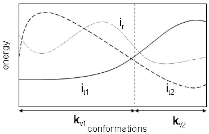
All possible conformations are divided into two subsets by fixing the rotamer of residue k to v1 or v2. For residue i the rotamer t1 dominates the rotamer r in the first subset of conformations. For the second subset, the rotamer t2 has a lower energy than r. Therefore, rotamer r which could not be eliminated by regular DEE, can be removed by split DEE.

In addition to the rotamer reduction method by DEE, many methods also use a residue reduction procedure, which eliminates residues with a single rotamer or with up to two interacting residues (neighbors). A residue with a single rotamer can be eliminated from further consideration by incorporating its pairwise energies into the self energies of its neighbors¹⁰¹. A residue with one neighbor can be reduced by adding its rotamer energies to the self-energies of its neighbor's rotamers¹⁰¹. A residue with two neighbors can be eliminated by updating the pairwise energies of the neighbors¹⁰⁶. The Residue-Rotamer-Reduction (R3) method¹⁰⁷ repeatedly performs residue and rotamer reduction. When a reduction is not possible in a certain iteration, the R3 method performs residue unification^{108, 103}. In this procedure, two residues are unified and a set of all their possible rotamer pairs is generated. The method finds the GMEC in a finite number of elimination iterations, because at least one residue is reduced in each iteration¹⁰⁷.

Bahadur et al.¹⁰⁹ have defined a weighted graph of non-colliding rotamers. In this graph the vertices are rotamers and two rotamers are connected by an edge if they represent different residues that do not have steric clashes. The weights on the edges correspond to the strength of the interaction between two rotamers. The algorithm searches for the maximum edge-weight clique in the induced graph. If the size of the obtained clique equals the number of residues, then each residue is assigned with exactly one rotamer. Since each two nodes in the clique are connected, none of the chosen rotamers collide. Thus, the obtained clique defines a feasible conformation and the maximum edge-weight clique corresponds to the GMEC.

The SCWRL¹⁰¹ algorithm uses a residue interaction graph in which residues with clashing rotamers are connected. The resulting graph is decomposed to biconnected components (seeFigure 7 (a, b)) and a dynamic programming technique is applied to find a GMEC. Any two components include at most one common residue - the articulation point. It starts by optimizing the leaf components, which have only one articulation point. The component's GMEC is calculated for each rotamer of the articulation point and is stored as the energy of the compatible rotamer for further GMEC calculations of adjacent components.Figure 7 (a, b) demonstrate the decomposition of a residue interaction graph into components. The drawback of the method is that it might include large components, which increase dramatically the CPU time. SCATD¹⁰⁶ proposes an improvement of the SCWRL methodology by using a tree decomposition of the residue interaction graph. This method results in more balanced decomposition and prevents creation of huge components, as opposed to biconnected decomposition. After this decomposition, any two components can share more than one common residue (Figure 7 c). Therefore, the component GMEC is calculated for every possible combination of these common residues and stored for further calculations.

Figure 7.

(a) Residue interaction graph. (b) SCWRL biconnected components: abcd and def with articulation point d. The SCWRL algorithm can start by optimizing the component def. For each rotamer of d, the GMEC of def is calculated while d is fixed. After this calculation the component def is collapsed into the rotamers of d. (c) SCATD tree decomposition. The articulation points are presented on the edges.

Recent methods use the mixed-integer linear programming (MILP) framework^{110, 111, 112, 113} to find a GMEC. In general, a decision variable is defined for each rotamer and rotamer-rotamer interaction. If a rotamer participates in GMEC, its corresponding decision variables will be equal to 1. Each decision variable is weighted by its score (self and pair-wise energies) and summed in a global linear expression for minimization. Constraints are set in order to guarantee one rotamer choice for each residue, and that only pair-wise energies between the selected rotamers are included in the global minimal energy. Although the MILP algorithm is NP-hard, by relaxation of the integrality condition on the decision variables, the polynomial-complexity linear programming algorithm can be applied to find the minimum. If the solution happens to be integral, the GMEC is found in polynomial time. Otherwise, an integer linear programming algorithm, with significantly longer running time, is applied. The MILP framework allows obtaining successive near-optimal solutions by addition of constraints that exclude the previously found optimal set of rotamers¹¹². The FireDock¹¹³ method for refinement and scoring of docking candidates uses the MILP technique for side-chain optimization. An example of a successful rotamer assignment by FireDock is shown inFigure 5(a).

In general, for all methods which use pair-wise energy calculations, a prefix tree data structure (trie) can be used for saving CPU time¹¹⁴. In a trie data structure, the inter-atomic energies of rotamers' parts, which share the same torsion angles, are computed once.

Many of the described methods efficiently find a GMEC due to the use of a simplified energy function, which usually includes only the repulsive van der Waals and rotamer probability terms. The energy function can be extended by additional terms, like the attractive van der Waals, solvation and electrostatics. However, this complicates the problem. The SCWRL/SCATD graph decomposition results in larger components, the number of decision variables in the MILP technique increases, etc. For example, Kingsford et al.¹¹² use only van der Waals and rotamer probability terms and almost always succeed in finding the optimal solution by polynomial LP. However, when adding electrostatic term, non-polynomial ILP is often required.

A performance comparison of R3¹⁰⁷, SCWRL¹⁰¹ and MILP¹¹² methods was performed^{107, 112}. The first test set included 25 proteins¹¹⁵. The differences in the prediction ability of the methods were minor, since they all find a GMEC and use a similar energy function. The time efficiency of the R3 and SCWRL methods was better than of MILP for these cases. The second test set of 5 proteins was harder¹⁰¹ and the R3 method performed significantly faster than SCWRL and MILP. In addition, Xu¹⁰⁶ demonstrated that the SCATD method shows a significant improvement in CPU time compared to SCWRL for the second test set.

4.2 Heuristic Methods for Treating Side-Chain Flexibility

Heuristic algorithms are widely used in side-chain refinement methods because of the following reasons. First, a continuous conformational space can be used during the minimization, as opposed to global optimization algorithms, where the conformational space has to be reduced to a pre-defined discrete set of conformers. Second, different energy functions can be easily incorporated into heuristic algorithms, while global optimization methods usually require a simplified energy function. A third advantage is that heuristic algorithms can provide many low-energy solutions, while most of the global algorithms provide a single one. However, the main drawback of the heuristic methods is that they cannot guarantee finding the GMEC.

Monte Carlo (MC)¹¹⁶ is an iterative method. At each step it randomly picks a residue and switches its current rotamer by another. The new overall energy is calculated and the conformational change is accepted or rejected by the Metropolis criterion¹¹⁷. In simulated annealing MC, the Boltzman temperature is high at the beginning to overcome local minima. Then, it is gradually lowered in order to converge to the global minimum. Finally, a quench step can be performed. The quench step cycles through the residues in a random order, and for each residue, the best rotamer for the overall energy is chosen. RosettaDock¹¹⁸ uses this rotamer-based MC approach and, in addition, performs gradient-based minimization in torsion space of dihedral angles.

The self-consistent mean-field (SCMF) optimization method ^{119, 120} uses a matrix which contains the probability of each rotamer to be included in the optimal solution. Each rotamer probability is calculated by the sum of its interaction energies with the surrounding rotamers, weighted by their respective probabilities. The method iteratively refines this matrix and converges in a few cycles. The 3D-DOCK¹²¹ package uses the mean-field approach for side-chain optimization with surrounding solvent molecules.

Other optimization techniques like genetic algorithms¹²² and neural networks¹²³ are also applied to predict optimal conformations of side-chains. Several methods do not restrict the conformational search to rotamers^{124, 125}. Abagyan et al.^{126, 125}(ICM-DISCO^{127, 128}) apply the biased probability MC method for minimization in the torsion angles space. Molecular dynamics simulations, described in Section 2.2, are also used to model flexibility of side-chains. SmoothDock^{129, 11} uses short MD simulations to predict conformations of anchor side-chains¹³⁰ at the pre-docking phase. HADDOCK^{32, 33} uses restricted MD simulations for final refinement with explicit solvent.

Obviously, an energy function has great influence on side-chain prediction performance. Yanover et al.¹³¹ showed that finding a GMEC does not significantly improve side-chain prediction results compared to the heuristic RosettaDock side-chain optimization. They showed that using an optimized energy function has much greater influence on the performance than using an improved search strategy.

Recent studies have shown that most of the interface residues do not undergo significant changes during binding^{130, 132, 64, 113}. Therefore, changing unbound conformations should be performed carefully during the optimization process^{118, 113}. In addition, when analyzing the performance of side-chain optimization methods, unbound conformations of side-chains should be used as a reference^{118, 113}.

5 Handling both backbone and side-chain flexibility in recent CAPRI challenges

In recent CAPRI (Critical Assessment of PRediction of Interactions) challenges¹³³, some of the participating groups attempted to handle both backbone and side-chain flexibility. Many groups treated conformational deformations by generating ensembles of conformations, which were later used for cross-docking. Additionally, some methods, specified below, handle protein flexibility during the docking process or in a refinement stage.

The group of Bates¹³⁴ used MD for generating ensembles of different conformations for the receptor and the ligand. Then, rigid body cross-docking was performed by the FTdock method⁷⁰. The best results were minimized by CHARMM¹³⁵, and clustered. Finally, a refinement by MD was performed. It has been shown that the cross-docking produced more near native results compared to unbound docking only in cases where the proteins undergo large conformational changes upon binding¹³⁴. Similar conclusions were obtained by Smith et al.⁶⁴.

The ATTRACT docking program^{136, 51} uses a reduced protein model, which represents each amino acid by up to three pseudo atoms. For each starting orientation, energy minimization is performed on six rigid-body degrees of freedom and on additional five degrees of freedom derived from the five lowest frequency normal modes. Finally the side-chain conformations at the interface of each docking solution are adjusted using the Swiss-PdbViewer¹³⁷, and the Sander program from the Amber8 package¹³⁸ is used for a final minimization.

The RosettaDock method^{94, 93} performs an initial low-resolution global docking, which includes a Monte Carlo (MC) search with random backbone and rigid-body perturbations. The low energy docking candidates are further refined by Monte-Carlo minimization (MCM). Each MCM cycle consists of: (i) backbone and/or rigid-body perturbation, (ii) rotamer-based side-chain optimization and (iii) quasi-Newton minimization on the degrees of freedom of the backbone and/or side-chains and/or rigid-body orientation.

The HADDOCK protocol³³ consists of rigid-body docking followed by a semi-flexible refinement of the interface in torsion angles' space (of both backbone and side-chains). As a final stage, a Cartesian dynamics refinement in explicit solvent is performed.

To conclude, the treatment of internal flexibility can be performed in different stages of the docking process and in different combinations. In many cases, backbone flexibility is treated before the side-chain flexibility. For example, an ensemble of backbone conformations is often created before the docking procedure. In addition, some methods, like ATTRACT and RosettaDock, perform backbone minimization prior to further refinement. There are two reasons for this order of handling flexibility: (i) the backbone deformations have greater influence on the protein structure than the side-chain movements; (ii) side-chain conformations often depend on the backbone torsion angles. On the other hand, in the final refinement stage, leading docking groups attempt to parallelize the treatment of all the degrees of freedom, including full internal flexibility and rigid-body orientation. CAPRI challenges still show unsatisfying results for cases with significant conformational changes. Therefore the optimal way to combine side-chain and backbone optimization methods is still to be found, and further work in this direction is required.

6 Discussion

Protein flexibility presents a great challenge in predicting the structure of complexes. This flexibility includes both backbone and side-chain conformational changes, which increase the size of the search space considerably. In this paper we reviewed docking methods that handle various flexibility types which are used in different stages of the docking process. These are summarized in the flowchart inFigure 8.Table I, Table II andTable III briefly specify the algorithmic approaches of these methods.

Figure 8.

A summary of methods for handling flexibility during docking, which are reviewed in the paper. The methods handle various flexibility types and are used in different stages of the docking process. Docking applications which implement the algorithmic methods are in brackets.

Table I.

Some Methods for Flexibility Analysis

Method	Flexibility Type	Description
DynDom17	Hinge bending	Given two conformations, cluster rotation vectors of short backbone segments and detects the rigid domains.
HingeFind18	Hinge bending	Compares given conformational states using sequence alignment and detects hinge locations.
FlexProt20, 21	Hinge bending	Compares given conformational states, pre-forms structural alignment and detects hinge locations.
HingeProt48	Hinge bending	Detects hinge locations using GNM.
CONCOORD61	General flexibility	Generate conformations that fulfill distance constraints.
Dynamite63	General flexibility	Generate conformations using the essential dynamics approach.
FIRST65	General flexibility	Identifies rigid and flexible substructures using Rigidity Theory.

Table II.

Some Methods for Docking with Backbone Flexibility

Method	Flexibility Type	Description
MC281	Flexible loops	Chooses the best loop conformations from an ensemble using the Mean-Field approach.
ATTRACT83, 51	Flexible loops	Chooses the best loop conformations from an ensemble using the Mean-Field approach.
	General flexibility	Energy minimization on degrees of freedom derived from the lowest frequency normal modes.
FlexDock86	Hinge bending	Allows hinge bending in the docking. The rigid subdomains are docked separately and consistent results are assembled.
FLIPDock92	General flexibility	Searches favored conformations by a genetic algorithm and a divide and conquer approach. Uses FT data structure.
HADDOCK32, 33	General flexibility	Handles backbone flexibility in the refinement stage, by simulated annealing MD.
RosettaDock10, 118, 93	General flexibility	Handles backbone flexibility in the refinement stage, by Monte Carlo minimization.

Table III.

Some Docking and Refinement Methods with Side-Chain and Rigid-Body Optimization

Method	Side-Chain Flexibility	Rigid-Body Optimization	Scoring Function Terms
RosettaDock10, 118, 93	MC on rotamers and minimization of rotamer torsion angles	MC with DFP quasi-Newton minimization147, 148	linear repVdW, attrVdW, EEF1 (SASA), rotamer probability, hydrogen bonds, residue pair potentials and electrostatics
ICM-DISCO128	biased probability MC on internal coordinates		truncated VdW, electrostatics, solvation, hydrogen bonds and hydrophobicity
3D-DOCK121	SCMF	steepest-descent minimization139	VdW, electrostatics and Langevin dipole solvation
SmoothDock129, 11	pre-docking MD and ABNR minimization in the refinement	simplex142 and ABNR minimization	VdW, electrostatics and ACE
HADDOCK32, 33	simulated annealing MD	steepest-descent minimization139	VdW, electrostatics, binding site restriction and buried surface area
RDOCK149	ABNR minimization		electrostatics and ACE
FireDock113	MILP	MC with BFGS quasi-Newton minimization150, 151	linear repVdW, attrVdW, ACE, electrostatics, π-stacking and aliphatic interactions, hydrogen and disulfide bonds and Insideness measure

The flexible docking process is divided into three major stages. In the first stage the flexibility of the proteins is analyzed. Hinge points can be detected by Ensemble Analysis, GNM or Rigidity Theory. Flexible loops can be identified by MD or Rigidity Theory. Additionally, general conformational space can be defined by NMA, MD or Essential Dynamics. In the second stage the actual docking is performed. If hinges were identified, the sub-domains can be docked separately. Furthermore, an ensemble of conformations can be generated, according to the results of the flexible analysis, and docked using cross-docking or the Mean Field approach. The docking candidates generated in this stage are refined in the third stage. This stage refines the backbone, side chains and rigid-body orientation. These three can be refined separately in an iterative manner or simultaneously. Backbone refinement can be performed by normal modes minimization. Side-chain optimization can be achieved by methods like MC, graph theory algorithms, MILP, and the Mean Field approach. The refinement of the orientation can be done by a variety of minimization methods such as Steepest Descent¹³⁹, Conjugate Gradient¹⁴⁰, Newton-Raphson, Quasi-Newton¹⁴¹ and Simplex¹⁴². Simultaneous refinement can be performed by methods like MD, MC and genetic algorithms. The final refined docking candidates are scored and ranked.

In spite of the variety of methods developed for handling protein flexibility during docking, the challenge is yet far from resolved. This can be observed from the CAPRI results^{143, 144, 133}, where in cases with significant conformational changes the predictions were dissatisfying. Modeling backbone flexibility is currently the main challenge in the docking field and is addressed by only a few methods. In contrast, side-chain flexibility is easier to model and encouraging results have been achieved. The rigid-body optimization stage plays an important role in flexible docking refinement, and contributes considerably to docking prediction success¹¹³. However, we believe that in order to achieve the best flexible refinement results, the refinement of the backbone, side-chains and rigid-body orientation need to be parallelized. Parallel refinement will best model the induced fit process that proteins undergo during their interaction.

Another major obstacle in the flexible docking field is the poor ranking ability of the current scoring functions. Adding degrees of freedom of protein flexibility to the search space increases the number of false-positive solutions. Therefore, a reliable energy function is critical for the correct model discrimination. The near-native solutions can be identified not only by their energies, but also by the existence of energy binding funnels^{11, 10}. Since the ranking ability of the current methods is dissatisfying, further work in this field is required.

Finally, we would like to emphasize that although modeling internal flexibility is essential for general docking predictions, rigid docking is also extremely important. In many known cases the structural changes that occur upon binding are minimal, and rigid-docking is sufficient^{145, 146}. The benefits of the rigid procedure are its simplicity and relatively low computational time. In addition, a reliable rigid docking algorithm is essential for generating good docking candidates for further flexible refinement.

Abbreviations

ABNR

A dopted Basis Newton-Raphson

ACE

Atomic Contact Energy

ANM

Anisotropic Network Model

DEE

Dead-End Elimination

FT

Flexible Tree

GMEC

Global Minimal Energy Conformation

GNM

Gaussian Network Model

MC(M)

Monte Carlo (Minimization)

MD

Molecular Dynamics

MILP

Mixed-Integer Linear Programming

NMA

Normal Modes Analysis

PCA

Principal Component Analysis

SASA

Solvent-Accessible Surface Area

SCMF

Self-Consistent Mean-Field

vdW

Van der Waals

References

- [1].Betts MJ, Sternberg MJ. An analysis of conformational changes on protein-protein association: implications for predictive docking. Protein Eng. 1999;12(4):271–283. doi: 10.1093/protein/12.4.271. [DOI] [PubMed] [Google Scholar]
- [2].Wodak SJ, Janin J. Computer analysis of protein-protein interactions. J. Mol. Biol. 1978;124:323–342. doi: 10.1016/0022-2836(78)90302-9. [DOI] [PubMed] [Google Scholar]
- [3].Halperin I, Ma B, Wolfson HJ, Nussinov R. Principles of docking: an overview of search algorithms and a guide to scoring functions. Proteins. 2002;47:409–442. doi: 10.1002/prot.10115. [DOI] [PubMed] [Google Scholar]
- [4].Marti-Renom MA, Stuart AC, Sanchez R, Fiser A, Melo F, Sali A. Comparative protein structure modeling of genes and genomes. Annu Rev Biophys Biomol Struct. 2000;29:291–325. doi: 10.1146/annurev.biophys.29.1.291. [DOI] [PubMed] [Google Scholar]
- [5].Soto CS, Fasnacht M, Zhu J, Forrest L, Honig B. Proteins. 2007. Loop modeling: sampling, filtering, and scoring. In press. [DOI] [PMC free article] [PubMed] [Google Scholar]
- [6].Grunberg R, Leckner J, Nilges M. Complementarity of structure ensembles in protein-protein binding. Structure. 2004;12(12):2125–2136. doi: 10.1016/j.str.2004.09.014. [DOI] [PubMed] [Google Scholar]
- [7].Tsai CJ, Ma B, Sham YY, Kumar S, Nussinov R. Structured disorder and conformational selection. Proteins. 2001;44(4):418–427. doi: 10.1002/prot.1107. [DOI] [PubMed] [Google Scholar]
- [8].James LC, Roversi P, Tawfik DS. Antibody multispecificity mediated by conformational diversity. Science. 2003;299(5611):1362–1367. doi: 10.1126/science.1079731. [DOI] [PubMed] [Google Scholar]
- [9].Goh CS, Milburn D, Gerstein M. Conformational changes associated with protein-protein interactions. Curr. Opin. Chem. Biol. 2004;14:1–6. doi: 10.1016/j.sbi.2004.01.005. [DOI] [PubMed] [Google Scholar]
- [10].Gray JJ, Moughon S, Schueler-Furman O, Kuhlman B, Rohl CA, Baker D. Protein-protein docking with simultaneous optimization of rigid-body displacement and side-chain conformations. J. Mol. Biol. 2003;331:281–299. doi: 10.1016/s0022-2836(03)00670-3. [DOI] [PubMed] [Google Scholar]
- [11].Camacho JC, Vajda S. Protein docking along smooth association pathways. Proc. Natl. Acad. Sci. USA. 2001;98:10636–10641. doi: 10.1073/pnas.181147798. [DOI] [PMC free article] [PubMed] [Google Scholar]
- [12].May A, Zacharias M. Accounting for global protein deformability during protein-protein and protein-ligand docking. Biochim Biophys Acta. 2005;1754:225–231. doi: 10.1016/j.bbapap.2005.07.045. [DOI] [PubMed] [Google Scholar]
- [13].Bonvin AM. Flexible protein-protein docking. Curr. Opin. Struct. Biol. 2006;16(2):194–200. doi: 10.1016/j.sbi.2006.02.002. [DOI] [PubMed] [Google Scholar]
- [14].Zeev-Ben-Mordehai T, Silman I, Sussman JL. Acetylcholinesterase in motion: visualizing conformational changes in crystal structures by a morphing procedure. Biopolymers. 2003;68(3):395–406. doi: 10.1002/bip.10287. [DOI] [PubMed] [Google Scholar]
- [15].Franklin J, Koehl P, Doniach S, Delarue M. MinActionPath: maximum likelihood trajectory for large-scale structural transitions in a coarse-grained locally harmonic energy landscape. Nucleic Acids Res. 2007;35(Web Server issue):W477–W482. doi: 10.1093/nar/gkm342. [DOI] [PMC free article] [PubMed] [Google Scholar]
- [16].Boutonnet NS, Rooman MJ, Wodak SJ. Automatic analysis of protein conformational changes by multiple linkage clustering. J. Mol. Biol. 1995;253:633–647. doi: 10.1006/jmbi.1995.0578. [DOI] [PubMed] [Google Scholar]
- [17].Hayward S, Berendsen HJ. Systematic analysis of domain motions in proteins from conformational change: new results on citrate synthase and T4 lysozyme. Proteins. 1998;30(2):144–154. [PubMed] [Google Scholar]
- [18].Wriggers W, Schulten K. Protein domain movements: detection of rigid domains and visualization of hinges in comparisons of atomic coordinates. Proteins. 1997;29(1):1–14. [PubMed] [Google Scholar]
- [19].Verbitsky G, Nussinov R, Wolfson HJ. Structural comparison allowing hinge bending, swiveling motions. Proteins. 1999;34:232–254. doi: 10.1002/(sici)1097-0134(19990201)34:2<232::aid-prot9>3.0.co;2-9. [DOI] [PubMed] [Google Scholar]
- [20].Shatsky M, Nussinov R, Wolfson HJ. FlexProt: alignment of flexible protein structures without a predefinition of hinge regions. J. Comp. Biol. 2004;11(1):83–106. doi: 10.1089/106652704773416902. [DOI] [PubMed] [Google Scholar]
- [21].Shatsky M, Nussinov R, Wolfson HJ. Flexible protein alignment and hinge detection. Proteins. 2002;48:242–256. doi: 10.1002/prot.10100. http://bioinfo3d.cs.tau.ac.il/FlexProt online available on. [DOI] [PubMed] [Google Scholar]
- [22].Schlick T. Molecular Modeling and Simulation, An Intersisciplinary Guide. Springer: 2002. [Google Scholar]
- [23].Di Nola A, Roccatano D, Berendsen HJC. Molecular dynamics simulation of the docking of substrates to proteins. Proteins. 1994;19:174–182. doi: 10.1002/prot.340190303. [DOI] [PubMed] [Google Scholar]
- [24].Mangoni M, Roccatano D, Di Nola A. Docking of flexible ligands to flexible receptors in solution by molecular dynamics simulation. Proteins. 1999;35:153–162. doi: 10.1002/(sici)1097-0134(19990501)35:2<153::aid-prot2>3.0.co;2-e. [DOI] [PubMed] [Google Scholar]
- [25].Pak Y, Wang S. Application of a molecular dynamics simulation method with a generalized effective potential to the flexible molecular docking problems. J. Phys. Chem. 2000;104:354–359. [Google Scholar]
- [26].Tsallis C. Possible generalization of boltzmanngibbs statistics. J. Stat. Phys. 1988;52:479–487. [Google Scholar]
- [27].Elber R. Long-timescale simulation methods. Curr. Opin. Struct. Biol. 2005;15(2):151–156. doi: 10.1016/j.sbi.2005.02.004. [DOI] [PubMed] [Google Scholar]
- [28].Schlick T, Barth E, Mandziuk M. Biomolecular dynamics at long timesteps: bridging the timescale gap between simulation and experimentation. Annu. Rev. Biophys. Biomol. Struct. 1997;26:181–222. doi: 10.1146/annurev.biophys.26.1.181. [DOI] [PubMed] [Google Scholar]
- [29].Chen J, Im W, Brooks CL., 3rd Application of torsion angle molecular dynamics for efficient sampling of protein conformations. J. Comput. Chem. 2005;26(15):1565–1578. doi: 10.1002/jcc.20293. [DOI] [PubMed] [Google Scholar]
- [30].Brunger AT, Adams PD, Rice LM. New applications of simulated annealing in x-ray crystallography and solution nmr. Structure. 1997;5(3):325–336. doi: 10.1016/s0969-2126(97)00190-1. [DOI] [PubMed] [Google Scholar]
- [31].Piela L, Kostrowicki J, Scheraga HA. On the multiple-minima problem in the conformational analysis of molecules: deformation of the potential energy hypersurface by the diffusion equation method. J. Phys. Chem. 1989;93(8):3339–3346. [Google Scholar]
- [32].Dominguez C, Boelens R, Bonvin A. HADDOCK: A protein-protein docking approach based on biochemical or biophysical information. J. Amer. Chem. Soc. 2003;125:1731–1737. doi: 10.1021/ja026939x. [DOI] [PubMed] [Google Scholar]
- [33].de Vries SJ, van Dijk AD, Krzeminski M, van Dijk M, Thureau A, Hsu V, Wassenaar T, Bonvin AM. HADDOCK versus HADDOCK: new features and performance of HADDOCK2.0 on the CAPRI targets. Proteins. 2007;69(4):726–733. doi: 10.1002/prot.21723. [DOI] [PubMed] [Google Scholar]
- [34].Riemann RN, Zacharias M. Refinement of protein cores and protein-peptide interfaces using a potential scaling approach. Protein Eng. Des. Sel. 2005;18(10):465–476. doi: 10.1093/protein/gzi052. [DOI] [PubMed] [Google Scholar]
- [35].Tai K. Conformational sampling for the impatient. Biophysical Chemistry. 2004;107:213–220. doi: 10.1016/j.bpc.2003.09.010. [DOI] [PubMed] [Google Scholar]
- [36].Grubmüller H. Predicting slow structural transitions in macromolecular systems: conformational flooding. Phys. Rev. E. 1995;52:2893. doi: 10.1103/physreve.52.2893. [DOI] [PubMed] [Google Scholar]
- [37].Lange OF, Schäfer LV, Grubmüller H. Flooding in GROMACS: accelerated barrier crossings in molecular dynamics. J. Comput. Chem. 2006;27(14):1693–1702. doi: 10.1002/jcc.20473. [DOI] [PubMed] [Google Scholar]
- [38].Rahman JA, Tully JC. Puddle-jumping: a flexible sampling algorithm for rare event system. Chemical Physics. 2002;285(2):277–287. [Google Scholar]
- [39].Tirion MM. Large amplitude elastic motions in proteins from a single-parameter, atomic analysis. Phys. Rev. Lett. 1996;77(9):1905–1908. doi: 10.1103/PhysRevLett.77.1905. [DOI] [PubMed] [Google Scholar]
- [40].Hinsen K. Analysis of domain motions by approximate normal mode calculations. Proteins. 1998;33:417–429. doi: 10.1002/(sici)1097-0134(19981115)33:3<417::aid-prot10>3.0.co;2-8. [DOI] [PubMed] [Google Scholar]
- [41].Ma J. New advances in normal mode analysis of supermolecular complexes and applications to structural refinement. Current Protein and Peptide Science. 2004;5:119–123. doi: 10.2174/1389203043486892. [DOI] [PMC free article] [PubMed] [Google Scholar]
- [42].Atilgan AR, Durell SR, Jernigan RL, Demirel MC, Keskin O, Bahar I. Anisotropy of fluctuation dynamics of proteins with an elastic network model. Biophys J. 2001;80:505–515. doi: 10.1016/S0006-3495(01)76033-X. [DOI] [PMC free article] [PubMed] [Google Scholar]
- [43].Petrone P, Pande VS. Can conformational change be described by only a few normal modes? Biophysical Journal. 2006;90:1583–1593. doi: 10.1529/biophysj.105.070045. [DOI] [PMC free article] [PubMed] [Google Scholar]
- [44].Tama F, Sanejouand YH. Conformational change of proteins arising from normal mode calculations. Protein Eng. 2001;14(1):1–6. doi: 10.1093/protein/14.1.1. [DOI] [PubMed] [Google Scholar]
- [45].Keskin O, Bahar I, Flatow D, Covell DG, Jernigan RL. Molecular mechanisms of chaperonin groel-groes function. Biochemistry. 2002;41(2):491–501. doi: 10.1021/bi011393x. [DOI] [PubMed] [Google Scholar]
- [46].Tama F, Brooks CL., 3rd The mechanism and pathway of pH induced swelling in cowpea chlorotic mottle virus. J. Mol. Biol. 2002;318(3):733–743. doi: 10.1016/S0022-2836(02)00135-3. [DOI] [PubMed] [Google Scholar]
- [47].Tama F, Valle M, Frank J, Brooks CL., 3rd Dynamic reorganization of the functionally active ribosome explored by normal mode analysis and cryo-electron microscopy. Proc. Natl. Acad. Sci. USA. 2003;100(16):9319–9323. doi: 10.1073/pnas.1632476100. [DOI] [PMC free article] [PubMed] [Google Scholar]
- [48].Emekli U, Schneidman-Duhovny D, Wolfson HJ, Nussinov R, Haliloglu T. Proteins. 2007. Hinge-Prot: Automated prediction of hinges in protein structures. In Press. [DOI] [PubMed] [Google Scholar]
- [49].Suhre K, Sanejouand YH. ElNemo: a normal mode web server for protein movement analysis and the generation of templates for molecular replacement. Nucleic Acids Res. 2004;32(Web Server issue):W610–W614. doi: 10.1093/nar/gkh368. [DOI] [PMC free article] [PubMed] [Google Scholar]
- [50].Tatsumi R, Fukunishi Y, Nakamura H. A hybrid method of molecular dynamics and harmonic dynamics for docking of flexible ligand to flexible receptor. J. Comput. Chem. 2004;25(16):1995–2005. doi: 10.1002/jcc.20133. [DOI] [PubMed] [Google Scholar]
- [51].May A, Zacharias M. Proteins. 2007. Energy minimization in low-frequency normal modes to efficiently allow for global flexibility during systematic protein-protein docking. In press. [DOI] [PubMed] [Google Scholar]
- [52].Cavasotto CN, Kovacs JA, Abagyan RA. Representing receptor flexibility in ligand docking through relevant normal modes. J. Amer. Chem. Soc. 2005;127(26):9632–40. doi: 10.1021/ja042260c. [DOI] [PubMed] [Google Scholar]
- [53].Mouawad L, Perahia D. Motions in hemoglobin studied by normal mode analysis and energy minimization: evidence for the existence of tertiary T-like, quaternary R-like intermediate structures. J. Mol. Biol. 1996;258(2) doi: 10.1006/jmbi.1996.0257. [DOI] [PubMed] [Google Scholar]
- [54].Miyashita O, Onuchic JN, Wolynes PG. Nonlinear elasticity, proteinquakes, and the energy landscapes of functional transitions in proteins. Proc. Natl. Acad. Sci. USA. 2003;100(22) doi: 10.1073/pnas.2135471100. [DOI] [PMC free article] [PubMed] [Google Scholar]
- [55].Tama F, Miyashita O, Brooks CL., 3rd Normal mode based flexible fitting of high-resolution structure into low-resolution experimental data from cryo-EM. J. Struct. Biol. 2004;147(3) doi: 10.1016/j.jsb.2004.03.002. [DOI] [PubMed] [Google Scholar]
- [56].Kirillova S, Cortes J, Stefaniu A, Simeon T. An NMA-guided path planning approach for computing large-amplitude conformational changes in proteins. Proteins. 2008;70(1) doi: 10.1002/prot.21570. [DOI] [PubMed] [Google Scholar]
- [57].Bahar I, Atilgan AR, Erman B. Direct evaluation of thermal fluctuations in proteins using a single-parameter harmonic potential. Fold Des. 1997;2:173–181. doi: 10.1016/S1359-0278(97)00024-2. [DOI] [PubMed] [Google Scholar]
- [58].Haliloglu T, Bahar I, Erman B. Gaussian dynamics of folded proteins. Physical review letters. 1997;79:3090–3093. [Google Scholar]
- [59].Amadei A, Linssen AB, Berendsen HJ. Essential dynamics of proteins. Proteins. 1993;17(4):412–425. doi: 10.1002/prot.340170408. [DOI] [PubMed] [Google Scholar]
- [60].Mustard D, Ritchie DW. Docking essential dynamics eigenstructures. Proteins. 2005;60(2):269–274. doi: 10.1002/prot.20569. [DOI] [PubMed] [Google Scholar]
- [61].de Groot BL, van Aalten DM, Scheek RM, Amadei A, Vriend G, Berendsen HJ. Prediction of protein conformational freedom from distance constraints. Proteins. 1997;29:240–251. doi: 10.1002/(sici)1097-0134(199710)29:2<240::aid-prot11>3.0.co;2-o. [DOI] [PubMed] [Google Scholar]
- [62].Mendez R, Leplae R, Lensink MF, Wodak SJ. Assessment of CAPRI predictions in rounds 3-5 shows progress in docking procedures. Proteins. 2005;60(2):150–169. doi: 10.1002/prot.20551. [DOI] [PubMed] [Google Scholar]
- [63].Barrett CP, Hall BA, Noble ME. Dynamite: a simple way to gain insight into protein motions. Acta Crystallogr. 2004;40:2280–2287. doi: 10.1107/S0907444904019171. [DOI] [PubMed] [Google Scholar]
- [64].Smith GR, Sternberg MJE, Bates PA. The relationship between the flexibility of proteins and their conformational states on forming protein-protein complexes with application to protein-protein docking. JMB. 2005;347:1077–1101. doi: 10.1016/j.jmb.2005.01.058. [DOI] [PubMed] [Google Scholar]
- [65].Jacobs DJ, Rader AJ, Kuhn LA, Thorpe MF. Protein flexibility predictions using graph theory. Proteins. 2001;44:150–165. doi: 10.1002/prot.1081. [DOI] [PubMed] [Google Scholar]
- [66].Jiang F, Kim SH. Soft docking: Matching of molecular surface cubes. J. Mol. Biol. 1991;219:79–102. doi: 10.1016/0022-2836(91)90859-5. [DOI] [PubMed] [Google Scholar]
- [67].Palma PN, Krippahl L, Wampler JE, Moura JG. BIGGER: A new (soft) docking algorithm for predicting protein interactions. Proteins. 2000;39:372–384. [PubMed] [Google Scholar]
- [68].Zacharias M. Protein-protein docking with a reduced protein model accounting for side-chain flexibility. Protein Sci. 2003;12(6):1271–1282. doi: 10.1110/ps.0239303. [DOI] [PMC free article] [PubMed] [Google Scholar]
- [69].Katchalski-Katzir E, Shariv I, Eisenstein M, Friesem AA, Aflalo C, Vakser IA. Molecular surface recognition: Determination of geometric fit between protein and their ligands by correlation techniques. Proc. Natl. Acad. Sci. USA. 1992;89:2195–2199. doi: 10.1073/pnas.89.6.2195. [DOI] [PMC free article] [PubMed] [Google Scholar]
- [70].Gabb HA, Jackson RM, Sternberg MJE. Modelling protein docking using shape complementarity, electrostatics, and biochemical information. J. Mol. Biol. 1997;272:106–120. doi: 10.1006/jmbi.1997.1203. [DOI] [PubMed] [Google Scholar]
- [71].Mandell JG, Roberts VA, Pique ME, Kotlovyi V, Mitchell JC, Nelson E, Tsigelny I, Eyck L.F. Ten. Protein docking using continuum electrostatics and geometric fit. Protein Eng. 2001;14:105–113. doi: 10.1093/protein/14.2.105. [DOI] [PubMed] [Google Scholar]
- [72].Chen R, Weng Z. Docking unbound proteins using shape complementarity, desolvation, and electrostatics. Proteins. 2002;47:281–294. doi: 10.1002/prot.10092. [DOI] [PubMed] [Google Scholar]
- [73].Chen R, Li L, Weng Z. Zdock: An initial-stage protein-docking algorithm. Proteins. 2003;52:80–87. doi: 10.1002/prot.10389. [DOI] [PubMed] [Google Scholar]
- [74].Eisenstein M, Katchalski-Katzir E. On proteins, grids, correlations, and docking. C R Biol. 2004;327(5):409–420. doi: 10.1016/j.crvi.2004.03.006. [DOI] [PubMed] [Google Scholar]
- [75].Gardiner EJ, Willett P, Artymiuk PJ. Protein docking using a genetic algorithm. Proteins. 2001;44:44–56. doi: 10.1002/prot.1070. [DOI] [PubMed] [Google Scholar]
- [76].Schneidman-Duhovny D, Nussinov R, Wolfson HJ. Predicting molecular interactions in silico II: protein-protein and protein-drug docking. Curr. Med. Chem. 2004;11(1):91–107. doi: 10.2174/0929867043456223. [DOI] [PubMed] [Google Scholar]
- [77].Duhovny D, Nussinov R, Wolfson HJ. Efficient unbound docking of rigid molecules. In: Guigo R, Gusfield D, editors. Workshop on Algorithms in Bioinformatics. Vol. 2452. Springer Verlag: 2002. pp. 185–200. [Google Scholar]
- [78].Norel R, Lin SL, Wolfson HJ, Nussinov R. Molecular surface complementarity at protein-protein interfaces: The critical role played by surface normals at well placed, sparse points in docking. J. Mol. Biol. 1995;252:263–273. doi: 10.1006/jmbi.1995.0493. [DOI] [PubMed] [Google Scholar]
- [79].Norel R, Lin SL, Wolfson HJ, Nussinov R. Shape complementarity at protein-protein interfaces. Biopolymers. 1994;34:933–940. doi: 10.1002/bip.360340711. [DOI] [PubMed] [Google Scholar]
- [80].Fischer D, Lin SL, Wolfson HJ, Nussinov R. A geometry-based suite of molecular docking processes. J. Mol. Biol. 1995;248:459–477. doi: 10.1016/s0022-2836(95)80063-8. [DOI] [PubMed] [Google Scholar]
- [81].Bastard K, Thureau A, Lavery R, Prevost C. Docking macromolecules with flexible segments. J. Comput. Chem. 2003;24(15):1910–20. doi: 10.1002/jcc.10329. [DOI] [PubMed] [Google Scholar]
- [82].Xu W, Rould MA, Jun S, Desplan C, Pabo CO. Crystal structure of a paired domain-DNA complex at 2.5 A resolution reveals structural basis for Pax developmental mutations. Cell. 1995;80(4):639–650. doi: 10.1016/0092-8674(95)90518-9. [DOI] [PubMed] [Google Scholar]
- [83].Bastard K, Prevost C, Zacharias M. Accounting for loop flexibility during protein-protein docking. Proteins. 2006;62(4):956–69. doi: 10.1002/prot.20770. [DOI] [PubMed] [Google Scholar]
- [84].Sandak B, Wolfson HJ, Nussinov R. Flexible docking allowing induced fit in proteins. Proteins. 1998;32:159–174. [PubMed] [Google Scholar]
- [85].Sandak B, Nussinov R, Wolfson HJ. A method for biomolecular structural recognition and docking allowing conformational flexibility. J. Comp. Biol. 1998;5(4):631–654. doi: 10.1089/cmb.1998.5.631. [DOI] [PubMed] [Google Scholar]
- [86].Schneidman-Duhovny D, Inbar Y, Nussinov R, Wolfson HJ. Geometry based flexible and symmetric protein docking. Proteins. 2005;60:224–231. doi: 10.1002/prot.20562. [DOI] [PubMed] [Google Scholar]
- [87].Schneidman-Duhovny D, Nussinov R, Wolfson HJ. Automatic prediction of protein interactions with large scale motion. Proteins. 2007;69(4):764–773. doi: 10.1002/prot.21759. [DOI] [PubMed] [Google Scholar]
- [88].Ben-Zeev E, Kowalsman N, Ben-Shimon A, Segal D, Atarot T, Noivirt O, Shay T, Eisenstein M. Docking to single-domain and multiple-domain proteins: old and new challenges. Proteins. 2005;60(2):195–201. doi: 10.1002/prot.20557. [DOI] [PubMed] [Google Scholar]
- [89].Fitzjohn PW, Bates PA. Guided docking: First step to locate potential binding sites. Proteins. 2003;52(1):28–32. doi: 10.1002/prot.10380. [DOI] [PubMed] [Google Scholar]
- [90].Lindahl E, Delarue M. Refinement of docked protein-ligand and protein-DNA structures using low frequency normal mode amplitude optimization. Nucleic Acids Res. 2005;33(14):4496–4506. doi: 10.1093/nar/gki730. [DOI] [PMC free article] [PubMed] [Google Scholar]
- [91].Zhao Y, Stoffler D, Sanner M. Hierarchical and multi-resolution representation of protein flexibility. Bioinformatics. 2006;22(22):2768–2774. doi: 10.1093/bioinformatics/btl481. [DOI] [PubMed] [Google Scholar]
- [92].Zhao Y, Sanner MF. FLIPDock: Docking flexible ligands into flexible receptors. Proteins. 2007;68(3):726–737. doi: 10.1002/prot.21423. [DOI] [PubMed] [Google Scholar]
- [93].Wang C, Bradley P, Baker D. Protein-protein docking with backbone flexibility. J. Mol. Biol. 2007 doi: 10.1016/j.jmb.2007.07.050. submitted. [DOI] [PubMed] [Google Scholar]
- [94].Chaudhury S, Sircar A, Sivasubramanian A, Berrondo M, Gray JJ. Incorporating biochemical information and backbone flexibility in RosettaDock for CAPRI rounds 6-12. Proteins. 2007;69(4):793–800. doi: 10.1002/prot.21731. [DOI] [PubMed] [Google Scholar]
- [95].Xiang Z, Soto CS, Honig B. Evaluating conformational free energies: the colony energy and its application to the problem of loop prediction. Proc. Natl. Acad. Sci. USA. 2002;99(11):7432–7437. doi: 10.1073/pnas.102179699. [DOI] [PMC free article] [PubMed] [Google Scholar]
- [96].Dunbrack RL, Jr., Karplus M. Backbone-dependent rotamer library for proteins. application to side-chain prediction. Journal of Molecular Biology. 1993;230(2):543–574. doi: 10.1006/jmbi.1993.1170. [DOI] [PubMed] [Google Scholar]
- [97].Pierce NA, Winfree E. Protein design is NP-hard. Protein Engineering. 2002;15(10):779–782. doi: 10.1093/protein/15.10.779. [DOI] [PubMed] [Google Scholar]
- [98].Chazelle B, Singh M, Kingsford CL. A semidefinite programming approach to side-chain positioning with new founding strategies. INFORMS J. Comput. 2003;16:308–392. [Google Scholar]
- [99].Reingold EM, Nievergelt J, Deo N. Combinatorial Algorithms. Theory and Practice. Prentice-Hall; New Jersey: 1977. [Google Scholar]
- [100].Gordon DB, Mayo SL. Branch-and-terminate: a combinatorial optimization algorithm for protein design. Structure. 1999;7(9):1089–1098. doi: 10.1016/s0969-2126(99)80176-2. [DOI] [PubMed] [Google Scholar]
- [101].Canutescu AA, Shelenkov AA, Dunbrack RL., Jr. A graph-theory algorithm for rapid protein side-chain prediction. Protein Sci. 2003;12(9):2001–2014. doi: 10.1110/ps.03154503. [DOI] [PMC free article] [PubMed] [Google Scholar]
- [102].Desmet J, De Maeyer M, Hazes B, Lasters I. The dead-end elimination theorem and its use in protein side-chain positioning. Nature. 1992;356(6369):539–542. doi: 10.1038/356539a0. [DOI] [PubMed] [Google Scholar]
- [103].Goldstein RF. Efficient rotamer elimination applied to protein side-chains and related spin glasses. Biophysical Journal. 1994;66(5):1335–1340. doi: 10.1016/S0006-3495(94)80923-3. [DOI] [PMC free article] [PubMed] [Google Scholar]
- [104].Pierce NA, Spriet JA, Desmet J, Mayo SL. Conformational splitting: A more powerful criterion for dead-end elimination. Journal of Computational Chemistry. 2000;21(11):999–1009. [Google Scholar]
- [105].Gordon DB, Hom GK, Mayo SL, Pierce NA. Exact rotamer optimization for protein design. Journal of Computational Chemistry. 2003;24(2):232–243. doi: 10.1002/jcc.10121. [DOI] [PubMed] [Google Scholar]
- [106].Xu J. Rapid protein side-chain packing via tree decomposition. Lecture Notes in Bioinformatics (Subseries of Lecture Notes in Computer Science) 2005;3500:423–439. [Google Scholar]
- [107].Xie W, Sahinidis NV. Residue-rotamer-reduction algorithm for the protein side-chain conformation problem. Bioinformatics. 2006;22(2):188–194. doi: 10.1093/bioinformatics/bti763. [DOI] [PubMed] [Google Scholar]
- [108].Desmet J, De Maeyer M, Lasters I. The Protein Folding Problem and Tertiary Structure Prediction. 1994. The dead-end elimination theorem: A new approach to the side-chain packing problem; pp. 307–337. [Google Scholar]
- [109].Bahadur KCD, Tomita E, Suzuki J, Akutsu T. Protein side-chain packing problem: A maximum edge-weight clique algorithmic approach. Journal of Bioinformatics and Computational Biology. 2005;3:103–126. doi: 10.1142/s0219720005000904. [DOI] [PubMed] [Google Scholar]
- [110].Eriksson O. Side chain-positioning as an integer programming problem. LNCS. 2001;2149:128–141. [Google Scholar]
- [111].Althaus E, Kohlbacher O, Lenhof HP, Muller P. A combinatorial approach to protein docking with flexible side chains. Journal of Computational Biology. 2002;9(4):597–612. doi: 10.1089/106652702760277336. [DOI] [PubMed] [Google Scholar]
- [112].Kingsford CL, Chazelle B, Singh M. Solving and analyzing side-chain positioning problems using linear and integer programming. Bioinformatics. 2005;21(7):1028–1036. doi: 10.1093/bioinformatics/bti144. [DOI] [PubMed] [Google Scholar]
- [113].Andrusier N, Nussinov R, Wolfson HJ. FireDock: Fast interaction refinement in molecular docking. Proteins. 2007;69(1):139–159. doi: 10.1002/prot.21495. [DOI] [PubMed] [Google Scholar]
- [114].Leaver-Fay A, Kuhlman B, Snoeyink J. WABI 2005. 2005. Rotamer-pair energy calculations using a trie data structure; pp. 389–400. [Google Scholar]
- [115].Xiang Z, Honig B. Extending the accuracy limits of prediction for side-chain conformations. Journal of Molecular Biology. 2001;311(2):421–430. doi: 10.1006/jmbi.2001.4865. [DOI] [PubMed] [Google Scholar]
- [116].Holm L, Sander C. Fast and simple monte carlo algorithm for side chain optimization in proteins: Application to model building by homology. Proteins: Structure, Function and Genetics. 1992;14(2):213–223. doi: 10.1002/prot.340140208. [DOI] [PubMed] [Google Scholar]
- [117].Metropolis N, Rosenbluth AW, Rosenbluth MN, Teller AH, Teller E. Equation of state calculations by fast computing machines. J. Chem. Phys. 1953;21:1087–1092. [Google Scholar]
- [118].Wang C, Schueler-Furman O, Baker D. Improved side-chain modeling for protein-protein docking. Protein Sci. 2005;14(5):1328–1339. doi: 10.1110/ps.041222905. [DOI] [PMC free article] [PubMed] [Google Scholar]
- [119].Koehl P, Delarue M. Application of a self-consistent mean field theory to predict protein side-chains conformation and estimate their conformational entropy. Journal of Molecular Biology. 1994;239(2):249–275. doi: 10.1006/jmbi.1994.1366. [DOI] [PubMed] [Google Scholar]
- [120].Mendes J, Soares CM, Carrondo MA. Improvement of side-chain modeling in proteins with the self-consistent mean field theory method based on an analysis of the factors influencing prediction. Biopolymers. 1999;50(2):111–131. doi: 10.1002/(SICI)1097-0282(199908)50:2<111::AID-BIP1>3.0.CO;2-N. [DOI] [PubMed] [Google Scholar]
- [121].Jackson RM, Gabb HA, Sternberg MJE. Rapid refinement of protein interfaces incorporating solvation: application to the docking problem. J. Mol. Biol. 1998;276:265–285. doi: 10.1006/jmbi.1997.1519. [DOI] [PubMed] [Google Scholar]
- [122].Tuffery P, Etchebest C, Hazout S, Lavery R. A new approach to the rapid determination of protein side chain conformations. J. Biomol. Struct. and Dyn. 1991;8(6):1267–1289. doi: 10.1080/07391102.1991.10507882. [DOI] [PubMed] [Google Scholar]
- [123].Hwang JK, Liao WF. Side-chain prediction by neural networks and simulated annealing optimization. Protein Eng. 1995;8(4):363–370. doi: 10.1093/protein/8.4.363. [DOI] [PubMed] [Google Scholar]
- [124].Lee C, Subbiah S. Prediction of protein side-chain conformation by packing optimization. J. Mol. Biol. 1991;217(2):373–388. doi: 10.1016/0022-2836(91)90550-p. [DOI] [PubMed] [Google Scholar]
- [125].Abagyan R, Totrov M. Biased probability monte carlo conformational searches and electrostatic calculations for peptides and proteins. J Mol Biol. 1994;235(3):983–1002. doi: 10.1006/jmbi.1994.1052. [DOI] [PubMed] [Google Scholar]
- [126].Fernandez-Recio J, Totrov M, Abagyan R. Soft protein-protein docking in internal coordinates. Protein Sci. 2002;11:280–291. doi: 10.1110/ps.19202. [DOI] [PMC free article] [PubMed] [Google Scholar]
- [127].Fernandez-Recio J, Totrov M, Abagyan R. ICM-DISCO docking by global energy optimization with fully flexible side-chains. Proteins. 2007;52(1):113–117. doi: 10.1002/prot.10383. [DOI] [PubMed] [Google Scholar]
- [128].Fernandez-Recio J, Totrov M, Abagyan R. Identification of protein-protein interaction sites from docking energy landscapes. J Mol Biol. 2004;335(3):843–865. doi: 10.1016/j.jmb.2003.10.069. [DOI] [PubMed] [Google Scholar]
- [129].Camacho CJ, Gatchell DW. Successful discrimination of protein interactions. Proteins. 2003;52(1):92–97. doi: 10.1002/prot.10394. [DOI] [PubMed] [Google Scholar]
- [130].Rajamani D, Thiel S, Vajda S, Camacho CJ. Anchor residues in protein-protein interactions. Proc. Natl. Acad. Sci. USA. 2004;101(31):11287–92. doi: 10.1073/pnas.0401942101. [DOI] [PMC free article] [PubMed] [Google Scholar]
- [131].Yanover C, Schueler-Furman O, Weiss Y. RECOMB 2007. 2007. Minimizing and learning energy functions for side-chain prediction; pp. 381–395. [DOI] [PubMed] [Google Scholar]
- [132].Li X, Keskin O, Ma B, Nussinov R, Liang J. Protein-protein interactions: hot spots and structurally conserved residues often locate in complemented pockets that pre-organized in the unbound states: implications for docking. J. Mol. Biol. 2004;344(3):781–795. doi: 10.1016/j.jmb.2004.09.051. [DOI] [PubMed] [Google Scholar]
- [133].Lensink MF, Wodak SJ, Mendez R. Docking and scoring protein complexes: CAPRI 3rd edition. Proteins. 2007;69(4):704–718. doi: 10.1002/prot.21804. [DOI] [PubMed] [Google Scholar]
- [134].Król M, Chaleil RA, Tournier AL, Bates PA. Implicit flexibility in protein docking: Cross-docking and local refinement. Proteins. 2007;69(4):750–757. doi: 10.1002/prot.21698. [DOI] [PubMed] [Google Scholar]
- [135].Brooks BR, Bruccoleri RE, Olafson BD, States DJ, Swaminathan S, Karplus K. CHARMM: A program for macromolecular energy, minimization, and dynamics calculations. J. Comput. Chem. 1983;4(2):187–217. [Google Scholar]
- [136].May A, Zacharias M. Protein-protein docking in CAPRI using ATTRACT to account for global and local flexibility. Proteins. 2007;69(5):774–780. doi: 10.1002/prot.21735. [DOI] [PubMed] [Google Scholar]
- [137].Guex N, Peitsch MC. SWISS-MODEL and the Swiss-PdbViewer: an environment for comparative protein modeling. Electrophoresis. 1997;18:2714–2723. doi: 10.1002/elps.1150181505. [DOI] [PubMed] [Google Scholar]
- [138].Case DA, Cheatham TE, III, Darden T, Gohlke H, Luo R, Merz KM, Jr., Onufriev A, Simmerling C, Wang B, Woods R. The Amber biomolecular simulation programs. J. Comput. Chem. 2005;26:1668–1688. doi: 10.1002/jcc.20290. [DOI] [PMC free article] [PubMed] [Google Scholar]
- [139].Arfken G. Mathematical Methods for Physicists. 3rd ed. Academic Press; Orlando, FL: 1985. [Google Scholar]
- [140].Hestenes MR, Stiefel E. Methods of conjugate gradients for solving linear systems. J. Research Nat. Bur. Standards. 1952;49:409–436. [Google Scholar]
- [141].Nocedal J, Wright SJ. Numerical Optimization. Springer-Verlag: 1999. [Google Scholar]
- [142].Nelder JA, Mead R. A simplex method for function minimization. The Computer Journal. 1965;7(4):308–313. [Google Scholar]
- [143].Smith GR, Fitzjohn PW, Page CS, Bates PA. Incorporation of flexibility into rigid-body docking: Applications in rounds 3-5 of CAPRI. Proteins. 2005;60(2):263–268. doi: 10.1002/prot.20568. [DOI] [PubMed] [Google Scholar]
- [144].Janin J, Wodak S. The third CAPRI assessment meeting Toronto, Canada, April 20-21, 2007. Structure. 2007;15(7):755–759. doi: 10.1016/j.str.2007.06.007. [DOI] [PubMed] [Google Scholar]
- [145].O'toole N, Vakser IA. Proteins. 2007. Large-scale characteristics of the energy landscape in protein-protein interactions. In press. [DOI] [PubMed] [Google Scholar]
- [146].Ruvinsky AM, Vakser IA. Proteins. 2007. Interaction cutoff effect on ruggedness of protein-protein energy landscape. In press. [DOI] [PubMed] [Google Scholar]
- [147].Davidon WC. AEC Research and Development Report, ANL-5990. 1959. Variable metric method for minimization. [Google Scholar]
- [148].Fletcher R, Powell MJD. A rapidly convergent descent method for minimization. Computer Journal. 1963;6(2):163–168. [Google Scholar]
- [149].Li L, Chen R, Weng Z. RDOCK: refinement of rigid-body protein docking predictions. Proteins. 2003;53(3):693–707. doi: 10.1002/prot.10460. [DOI] [PubMed] [Google Scholar]
- [150].Broyden CG. The convergence of a class of double-rank minimization algorithms. Journal of the Institute of Mathematics and its Applications. 1970;6:76–90. [Google Scholar]
- [151].Fletcher R. A new approach to variable metric algorithms. The Computer Journal. 1970;13(3):317–322. [Google Scholar]