Signaling cascades as cellular devices for spatial computations

Abstract

Signaling networks usually include protein-modification cycles. Cascades of such cycles are the backbones of multiple signaling pathways. Protein gradients emerge from the spatial separation of opposing enzymes, such as kinases and phosphatases, or guanine nucleotide exchange factors (GEFs) and GTPase activating proteins (GAPs) for GTPase cycles. We show that different diffusivities of an active protein form and an inactive form leads to spatial gradients of protein abundance in the cytoplasm. For a cascade of cycles, using a discrete approximation of the space, we derive an analytical expression for the spatial gradients and show that it converges to an exact solution with decreasing the size of the quantization. Our results facilitate quantitative analysis of the dependence of spatial gradients on the network topology and reaction kinetics. We demonstrate how different cascade designs filter and process the input information to generate precise, complex spatial guidance for multiple GTPase effector processes. Thus, protein-modification cascades may serve as devices to compute complex spatial distributions of target proteins within intracellular space.

Introduction

Intracellular signaling processes, which convey signals from cell-surface receptors to target genes in the nucleus, have a spatial as well as the (usually studied) temporal dimension. The signals received at the cell membrane need to be transported across the cell interior, and active transport or diffusion can therefore influence the input-output characteristics of signal transduction processes [1]. In addition, pivotal processes such as cell division, polarization and migration depend on the generation and processing of intracellular signals that monitor the relative localization of cellular components, either in relation to other components or to external cues. For instance, in mitosis the spindle-positioning checkpoint surveys the position of chromosomes during their distribution and delays cytokinesis until proper spindle positioning is attained [2].

Spatial separation of two opposing enzymes in a protein modification cycle was predicted to create patterns of positional information within a cell [3]. In particular, protein phosphorylation / dephosphorylation and GTPase activation / inactivation cycles can generate spatial (activity) gradients. Such a protein modification cycle for GTPases is shown in Fig. 1. For instance, if phosphorylation of a diffusible target protein is catalyzed by a kinase localized to a scaffold, supramolecular structure or the membrane, whereas the opposing phosphatase is homogeneously dispersed, spatial gradients of the protein phosphorylation state can occur. This reaction-diffusion system generates a high level of phosphorylation of the target protein in the close vicinity of the scaffold or near the membrane and a low phosphorylation level at distant cytoplasmic areas [3, 4]. Steadily changing gradients generate the spatial information, which guides the processes that depend on the phosphorylation or activity state of the diffusible target protein.

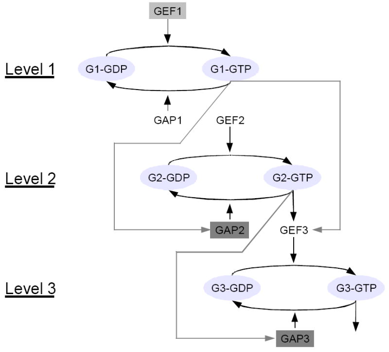
Figure 1.

Network scheme for a three-level GTPase cascade. The grey box comprises the components participating in a single (the first) level of the cascade, namely a guanine nucleotide exchange factor (GEF) and a corresponding GTPase activating protein (GAP) that catalyze the conversion of GTPase-GDP to GTPase-GTP (abbreviated by Gi-GDP and Gi-GTP) and vice-versa, respectively. In addition, GTPases have (low) intrinsic GTP-hydrolyzing activities (not shown). The network includes three such modules. They are connected through sequential activation of the GEFs for levels 2 and 3 by the active GTPases of the corresponding previous levels.

New experimental methods for detecting activity states of certain proteins in living cells recently lead to an experimental observation of the predicted activity gradients. For instance, fluorescence resonance energy transfer-based biosensors enabled the detection of gradients of the small GTPases Cdc42 [5] and Ran [6-8] as well as of phosphorylated stathmin, a microtubule-binding protein [9]. With suitable probes, even highly unstable enzyme-substrate complexes can nowadays be monitored with sub-cellular spatial resolution [10]. These studies have revealed that spatial gradients of signaling molecules play important roles in the spatial coordination of cell division processes, which often employ small GTPases to generate spatial ‘clues’ [11].

Biochemical and genetic studies have provided evidence that different types of GTPases interact in processes linked to spatial sensing. For instance, the interactions between a Ras and a Rho GTPase couple the selection of a growth site to the development of cell polarity in yeast [12]. Likewise, many real cellular signaling networks are more complex than a single protein modification cycle [13]. Networks of small GTPases involved in cell polarity and movement, when modeled as reaction-diffusion systems show that realistic representations of complex spatial processes, in principle, can be obtained [14]. However, beyond numerical simulation, a more fundamental understanding of the qualitative behavior of cell signaling in space is currently lacking.

In this paper, we aim at investigating possible mechanisms of signal generation and propagation using reaction-diffusion models. We start with single-protein modules and extend the analyses to cascades of interacting proteins in order to reveal general features of signaling processes in space. We demonstrate that different diffusivities of active and inactive protein forms can lead to spatial gradients of protein abundance (the local sum of all modulation states of that protein) in the cytoplasm. We show how GTPase cascades can process and encode input information into complex, non-monotonic spatial profiles of the GTPase activity gradients.

Spatial gradients in single-protein modules

Activity gradients by reaction-diffusion processes

The development of imaging techniques allowed direct experimental observation of activity gradients in the control of the mitotic spindle [6, 8]. This process involves the diffusible small GTPase Ran. Ran-GDP is activated by the guanine nucleotide exchange factor (GEF) RCC1, which is predominantly bound to chromosomes [15]. In contrast, the hydrolysis of Ran-GTP is catalyzed by RanGAP1 that is homogeneously distributed in the surrounding area [6, 16] (see Fig. 2). When the diffusivities (D) of active Ran-GTP (c) and inactive Ran-GDP (c_I) are the same, this reaction-diffusion system can be described as follows,

Figure 2.

The Ran system for control of the mitotic spindle. Spatial separation of the opposing enzymes, GEF RCC1 and RanGAP1, generates intracellular gradients of the small GTPase Ran. RCC1 localizes to chromosomes, whereas RanGAP1 is homogeneously distributed in the cytoplasm. The concentration gradients are shown by colour intensity. The characteristic length of the gradient is determined by the RanGAP1 activity and the Ran diffusivity (Eq. (3)).

$$\frac{\partial c}{\partial t}=D\mathrm{\Delta }c-v_I\hspace{0.17em}(c),\hspace{0.17em}c+c_I=c^{\mathit{tot}}$$ (1)

Here v_I is the rate of RanGAP1-catalyzed GTP-hydrolysis, i.e. the rate of GTPase inactivation. The total Ran concentration, c^tot, is constant at each space and time point on the time scale of the signal transfer [4]. In order to make analytical estimates, we assume a spherical symmetry (Fig. 2) and that the RanGAP1 activity is far from saturation, i.e., v_I(c) = k_I c (k_I= V_max/K_m is the observed first-order rate constant). The space geometry considered is the following: the Ran activator, RCC1, is bound to a chromatin structure of the radius s, and the opposing enzyme RanGAP1 is dispersed in the surrounding area of the radius M. Then, the steady state Ran-GTP concentration c(r) is determined by [3],

$$\frac{D}{r^2}\frac{\partial }{\partial r}\left(r^2\frac{\partial c}{\partial r}\right)-k_{I}c=0,\hspace{0.17em}-D\frac{\partial c}{\partial r}{|}_{r=s}=v_A,\hspace{0.17em}\frac{\partial c}{\partial r}{|}_{r=M}=0,$$ (2)

where v_A is the GEF-catalyzed GTP exchange rate at the surface of the chromatin structure. The analytical solution to this equation gives the ratio of the Ran-GTP concentration at the distance (r-s) from the chromosome to the Ran-GTP concentration at the chromosome surface (r = s),

$$\frac{c(r)}{c(s)}=e^{-\alpha (r-s)}\cdot \frac{s}{r}\cdot \left(\frac{e^{2\alpha r}(\alpha M+1)+e^{2\alpha M}(\alpha M-1)}{e^{2\alpha s}(\alpha M+1)+e^{2\alpha M}(\alpha M-1)}\right),\hspace{0.17em}{\alpha }^2=\frac{k_I}{D}$$ (3)

Eqn. (3) shows that Ran-GTP decreases roughly exponentially with the distance (r-s) from the chromosome. The characteristic length of the Ran-GTP gradient is determined as [3, 17],

$$L=\sqrt{D/k_I}$$ (4)

Since the diffusivity of Ran is 20 μm²/s and the k_I value is in the range of 0.5 - 5 s^-1, the Ran-GTP gradient appears to be precipitous with the characteristic length of 2 - 6 μm [6, 16], as indeed was measured experimentally [8]. Similar characteristic length and nearly exponential form of the protein activity gradients were first reported for the different geometry where protein is activated at the membrane of a spherical cell and diffuses in the cell interior where it is deactivated [3]. This approximation holds true if the deactivating enzyme is homogeneously distributed in the cytoplasm and operates far from saturation. Note that the analytical solution can also be obtained readily for the fully saturated condition [17]. Using discretization of the space, in this paper we derive the analytical solution for a cascade of cycles and for arbitrary kinetics of activating and deactivating enzymes. This allows us to explore multiple interaction motifs of the GTPase cascades and demonstrate how different spatial signals are processed and controlled by these cascades.

In a general case, a source of active GTPase can be on many cellular membranes, including the plasma membrane and the Golgi apparatus [18]. In the case of spherical symmetry, the steady state solutions to reaction-diffusion equations for a 3-dimensional system (Eqs. (2) and (3)) have many similarities with solutions to a one-dimensional system (see below). Without loss of generality, we will further consider a one-dimensional system with Cartesian spatial coordinate x, where we assume that the GTPase is activated at a source x=0, can freely diffuse, and is converted to inactive GDP-bound form. With identical diffusion coefficients D for both forms of the GTPase, the stationary profile of activated GTPase c(x) is described by

$$k_I\cdot c(x)-D\cdot \frac{{\partial }^{2}c(x)}{\partial x^2}=0$$ (5)

with the specific GTP hydrolysis rate constant k_I. To model the source, one can either assume a fixed concentration c₀ of active GTPase at the boundary x =0,

$$c(0)=c_0$$ (6)

or postulate that the rate of the surface-reaction (the GEF-catalyzed activation with rate constant k_A) equals the diffusive flux:

$$-D\frac{\partial c}{\partial x}{|}_{x=0}=v_A$$ (7)

For both scenarios, using a Neumann (zero flux) condition for the other system boundary at x_L

$$\frac{\partial c(x)}{\partial x}{|}_{x=x_L}=0$$ (8)

we obtain an analytical solution of the form

$$c(x)=c_0\left(\frac{\exp (-\varphi x_L(2-x/x_L))+\exp (-\varphi x)}{1+\exp (-2\varphi x_L)}\right),\hspace{0.17em}\varphi =\sqrt{k_I/D}$$ (9)

with the gradient’s characteristic length L = 1/φ (see Eq. (4)). For large φ and/or large x_L, thus, again c(x) ≈ c₀ · exp(−φ·x). Note that for the fixed-concentration boundary condition (Eq. (6)), the GEF activity at x=0 does not control the activation level of the GTPase near the source point (c₀), whereas in the second scenario (Eq. (7)) only c₀ depends on the GEF activity.

Emergence of spatial gradients of protein abundances within cells

Spatial gradients of protein abundance within a cell can emerge when the diffusivities of an active (for instance, phosphorylated) form and an inactive (unphosphorylated) form are different. In fact, the active form of a signaling protein often interacts with other proteins and generates multi-protein complexes. The Stokes radius of a complex can be much larger than the radius of the original, inactive form. According to the Einstein-Stokes equation, this can lead to a significant decrease in the diffusion coefficient of the active form, provided that the complex is sufficiently stable, and therefore the total residence time of the active form in the complex is large. The Einstein-Stokes equation for the diffusion coefficient reads,

$$D=\frac{k_{B}T}{6\pi \eta S}$$ (9),

where k_B is the Boltzmann’s constant, T is the absolute temperature, η is the viscosity of the medium, and S is the Stokes radius, which is roughly proportional to the cube root of the molecular weight (MW). Therefore, if an active form of a low MW protein associates with a high MW protein, or forms a multi-protein complex, the diffusion coefficient of the complex will be considerably less than the diffusivity of an inactive form.

In contrast with a general case for the GTPase system described by Eq. (5), we will need two separate equations to account for the dynamics of phosphorylated and unphosphorylated forms, as their sum will now depend on the spatial coordinate. In addition, we will not make any a priori assumption about the kinetics of the membrane kinase and diffusible phosphatase. Assuming that the association of the phosphorylated form (c) with other proteins does not protect this form against the phosphatase activities, the spatio-temporal behavior of phosphorylated form and inactive, unphosphorylated form (c_I) will be described by the reaction diffusion system with similar reaction terms, but different diffusivities, D and D_I, respectively. For illustrative purposes, we consider the simplest one-dimensional (1-D) geometry, and all results apply readily to a 3-D case. This simplest 1-D geometry corresponds to a cylindrical bacterial cell of the length H. We will assume that a kinase is localized to the membrane at a single pole of this cell (at the spatial coordinate x = 0) and a phosphatase is distributed in the cytoplasm. The kinase rate v_A is defined as the surface-rate at x = 0 . The phosphorylated protein (c) diffuses into the cell and gets dephosphorylated by the phosphatase at rate v_I. The spatio-temporal dynamics of the phosphorylated protein form c and of the unphosphorylated form c_I of the interconvertible protein are governed by the following reaction-diffusion equations,

$$\frac{\partial c}{\partial t}=D\frac{{\partial }^{2}C}{\partial x^2}-v_I\hspace{0.17em}(c)$$

$$\frac{\partial c_I}{\partial t}=D_I\hspace{0.17em}\frac{{\partial }^2{c}_I}{\partial x^2}+v_I\hspace{0.17em}(c)$$ (10)

The boundary conditions are the following,

$$-D\frac{\partial c}{\partial x}{|}_{x=0}=D_I\frac{\partial c_I}{\partial x}{|}_{x=0}=v_A;\hspace{0.17em}\frac{\partial c}{\partial x}{|}_{x=H}=\frac{\partial c_I}{\partial x}{|}_{x=H}=0$$ (11)

In contrast to the previous section, here we allow for any functional form of the phosphatase rate v_I. In this general case, the following can be derived. At the steady state, the time derivatives are zero, and from Eq. (10), it follows,

$$D\frac{{\partial }^{2}c}{\partial x^2}+D_I\hspace{0.17em}\frac{{\partial }^2{c}_I}{\partial x^2}=0$$ (12)

Integrating Eq. (12) from 0 to x, and taking into account the boundary conditions, Eq. (11), we have,

$$D\frac{dc}{dx}+D_I\hspace{0.17em}\frac{d{c}_I}{dx}=D{\frac{dc}{dx}|}_{x=0}+D_I\hspace{0.17em}{\frac{d{c}_I}{dx}|}_{x=0}=0$$ (13)

Finally, integrating Eq. (13) from 0 to x and rearranging, we obtain,

$$D(c(0)-c(x))=D_I\hspace{0.17em}(c_I\hspace{0.17em}(x)-c_I\hspace{0.17em}(0)),$$ (14)

Since the diffusivity D of the phosphorylated form is smaller than the diffusivity D_I of inactive protein, D < D_I, the phosphoprotein gradient Grad_p ≡ c(0) − c(x) is more precipitous than the gradient Grad_I ≡ c_I(x) − c_I(0) of the unphosphorylated protein,

$${\mathit{Grad}}_p/{\mathit{Grad}}_I=D_I/D\ge 1.$$

Importantly, Eq. (14) shows that the difference in the diffusivities D and D_I brings about the spatial gradient, Grad^tot, of the protein abundance,

$$c^{\mathit{tot}}(x)=c(x)+c_I\hspace{0.17em}(x),$$

$${\mathit{Grad}}^{\mathit{tot}}=c^{\mathit{tot}}(0)-c^{\mathit{tot}}(x)=\left(1-\frac{D}{D_I}\right)\hspace{0.17em}(c(0)-c(x))=\left(1-\frac{D}{D_I}\right)\hspace{0.17em}{\mathit{Grad}}_p$$ (15)

With realistic parameter values, pronounced spatial gradients in protein abundance appear (Fig. 3). We conclude that precipitous gradients of the phosphorylated form may lead to inhomogeneous spatial distribution of the total number of molecules of the target protein, if the diffusivities of active and inactive forms are different.

Figure 3.

Spatial gradients of protein abundance for the phosphorylated form (c, dashed line), unphosphorylated form (c_I, dotted line), and total protein (c^tot, solid line). We used Eqs. (9) and (15) to compute the gradient for c. Parameters were set to realistic values for the Ran system, namely D = 10 μm² s^-1, D_I = 20 μm² s^-1, k_I = 5 s^-1. Concentrations are normalized such that c(x=0) = 2 a.u. and c_I(x=0) = 1 a.u.

Suppose that the association of the active form of the target protein with another protein protects this form from deactivation by the opposing enzyme in the cytoplasm. For instance, the binding of Ran-GTP to importin-β prevents the GTP hydrolysis catalyzed by RanGAP, extending the characteristic length of the gradient of the Ran-GTP-importin-β complex [6]. However, even in this case the gradient of the total Ran concentration will occur within the cell. The sum of the free Ran-GTP and Ran-GDP concentrations remains constant, as their diffusivities are the same, whereas the emerging gradient of the Ran-GTP-importin-β complex results in the gradient of the Ran abundance in the cell.

Spatial gradients in protein cascades

Quantized reaction-diffusion model for GTPase cascades

To extend the simple models for a single gradient to more complicated signaling processes, we will consider signaling cascades, where GTPases at each cascade level positively or negatively control GEFs or GAPs for GTPases at subsequent levels. According to the model scenarios, the systems’ components can freely diffuse or are localized to specific membranes or cell structures. Moreover, the transitions from the active GTP-bound form to the inactive GDP-bound form can occur with or without associated GAP. To establish a corresponding, generalized model, we assume that the spatial distribution of GEFs and GAPs can be approximated by discrete values. More specifically, we consider a one-dimensional spatially distributed system with Cartesian spatial coordinate x that is sub-divided into N sections. These sections may, but do not need to correspond to cell compartments such as the membrane or nucleus. Individual GEF and GTPase reactions may be assigned to each section. The corresponding N + 1 positions of section boundaries are x_k with k ∈ {0,…,N}.

Similar to the simple version of the single-GTPase system (see the previous section, Eq. (5)), we will assume equal diffusion coefficients (D) for GTP- and GDP-bound GTPases. Then, the stationary profile of active GTPase c_i(x) in section i ∈ {1,…,N} can be described by

$$-v_I\hspace{0.17em}(i)\cdot c_i\hspace{0.17em}(x)+v_A\hspace{0.17em}(i)\cdot [c^{\mathit{tot}}-c_i\hspace{0.17em}(x)]+D\cdot \frac{{\partial }^2{c}_i\hspace{0.17em}(x)}{\partial x^2}=0$$ (16)

Note that the GTP hydrolysis rates v_I(i) and the GTP exchange rates v_A(i) are now defined specifically for each section. This allows for a discrete approximation of the effects that GTPases may exert on each other provided there are no feedback loops. Moreover, the reaction rate laws v_I(i) and v_A(i) can be arbitrary functions of the system’s components.

For continuity at the borders between sections, concentrations and fluxes at each side of an interior border n ∈ {1,…,N − 1} have to be identical, that is,

$$c_n(x){|}_{x_n}=c_{n+1}(x){|}_{x_n};\hspace{0.17em}\frac{\partial c_n(x)}{\partial x}{|}_{x_n}={\frac{\partial c_{n+1}(x)}{\partial x}|}_{x_n}\cdot$$ (17)

Furthermore, we consider a closed system [x₀ , x_N] with Neumann boundary conditions, which implies

$$\frac{\partial c_1\hspace{0.17em}(x)}{\partial x}{|}_{x_0}=\frac{\partial c_N\hspace{0.17em}(x)}{\partial x}{|}_{x_N}=0$$ (18)

The solution of PDE (16) has the following form:

$$c_i(x)=\alpha (i)\cdot \exp (-\varphi (i)\cdot x)+\beta (i)\cdot \exp (+\varphi (i)\cdot x)+\xi (i),$$ (19)

where the characteristic length scale 1/ L(j) = φ(j) and the constant term ξ(j) are given by $\varphi (j)=\sqrt{\frac{v_I\hspace{0.17em}(j)+v_A\hspace{0.17em}(j)}{D}}$ and $\xi (j)=\frac{c^{\mathrm{tot}}\cdot v_A\hspace{0.17em}(j)}{v_I\hspace{0.17em}(j)+v_A\hspace{0.17em}(j)}$, respectively. For determining the parameters a(i) and β(i), continuity and boundary conditions (17)-(18) yield

$$\beta (1)\cdot g{(1,0)}^2-\alpha (1)=\beta (N)\cdot g{(N,N)}^2-\alpha (N)=0$$

$$\alpha (n)\cdot f(n,n)+\beta (n)\cdot g(n,n)+\xi (n)=\alpha (n+1)\cdot f(n+1,n)+\beta (n+1)\cdot g(n+1,n)+\xi (n+1)$$

$$\varphi (n)[\beta (n)\cdot g(n,n)-\alpha (n)\cdot f(n,n)]=\varphi (n+1)[\beta (n+1)\cdot g(n+1,n)-\alpha (n+1)\cdot f(n+1,n)]$$ (20)

Here, to simplify the notation we have defined two auxiliary functions f(j,k) and g(j,k) as

$$f(j,k)=\exp (-\varphi (j)\cdot x_k);\hspace{0.17em}g(j,k)=f{(j,k)}^{-1}=\exp (+\varphi (j)\cdot x_k).$$ (21)

Elimination of β(n) and α(n) in Eqns. (20) leads to

$$\alpha (n)={\gamma }_{1,1}(n)\cdot \alpha (n+1)+{\gamma }_{1,2}(n)\cdot \beta (n+1)+{\gamma }_{1,3}(n)$$

$$\beta (n)={\gamma }_{2,1}(n)\cdot \alpha (n+1)+{\gamma }_{2,2}(n)\cdot \beta (n+1)+{\gamma }_{2,3}(n)$$ (22)

with

$${\gamma }_{1,1}(n)=\delta (n)\cdot f(n+1,n)\cdot g(n,n);{\gamma }_{2,1}(n)=[1-\delta (n)]\cdot f(n+1,n)\cdot f(n,n)$$

$${\gamma }_{1,2}(n)=[1-\delta (n)]\cdot g(n+1,n)\cdot g(n,n);{\gamma }_{2,2}(n)=\delta (n)\cdot g(n+1,n)\cdot f(n,n)$$

$${\gamma }_{1,3}(n)=\epsilon (n)\cdot g(n,n);{\gamma }_{2,3}(n)=\epsilon (n)\cdot f(n,n)$$

$$\delta (n)=1/2[\varphi (n+1)/\varphi (n)+1];\epsilon (n)=1/2[\xi (n+1)-\xi (n)].$$ (23)

By successive elimination of the α(n+1), β(n+1) in the 2(N−1) equations (20) and (22), we obtain for coefficient β(N) in the final section

$$\beta (N)=\frac{{\sum }_{j=1}^{N-1}\left({\mathrm{\Gamma }}_{1,3}(j)-g{(1,0)}^2\cdot {\mathrm{\Gamma }}_{2,3}(j)\right)}{g{(1,0)}^2\hspace{0.17em}\left[g{(N,N)}^2\cdot {\mathrm{\Gamma }}_{2,1}(N-1)+{\mathrm{\Gamma }}_{2,2}(N-1)\right]-g{(N,N)}^2\cdot {\mathrm{\Gamma }}_{1,1}(N-1)-{\mathrm{\Gamma }}_{1,2}(N-1)}$$ (24)

employing an auxiliary function Γ_j,k (l) (j ∈ {1,2},k ∈ {1,2,3}) defined by

$${\mathrm{\Gamma }}_{j,k}\hspace{0.17em}(l)=\{\begin{array}{ccc}{\gamma }_{j,k}\hspace{0.17em}(l)& \mathrm{for}& l=1\\ {\gamma }_{1,k}\hspace{0.17em}(l)\cdot {\mathrm{\Gamma }}_{j,1}\hspace{0.17em}(l-1)+{\gamma }_{2,k}\hspace{0.17em}(l)\cdot {\mathrm{\Gamma }}_{j,2}\hspace{0.17em}(l-1)& \mathrm{for}& 2\le l\le N-1\end{array}.$$ (25)

All other coefficients a(i) and β(i) can be calculated recursively from Eqns. (20)-(23). Note that for numerical accuracy, slightly different implementations are advantageous (e.g., replacing products of exponential functions by single variables).

Accuracy of the quantized model

First, we sought to assess the accuracy of the above GTPase model with spatial quantization. In this model, the GTP hydrolysis rates v_I(i) and the GTP exchange rates v_A(i) are section-specific to account for spatial heterogeneity of input signals such as GEF and GAP activities. For simple gradients, one can obtain analytical solutions for the reaction-diffusion system where the reaction rates are continuous functions in space (i.e. PDE (16) and boundary conditions (18), omitting the index i). We can, thus, evaluate the accuracy of the quantized model against such a simple case. Here, we consider a linear gradient of GEF activity but spatially homogeneous GTP hydrolysis rates, that is,

$$v_I^c(x)=k_{\mathit{GTPase}},\hspace{0.17em}{v}_A^c(x)=k_{\mathit{GEF}}\cdot x$$ (26)

where superscripts c denote that the rates are continuous functions of the spatial coordinate x. For the quantized model, we employed a discrete approximation of the GEF gradient, namely the activity at the midpoint of each interval. Correspondingly, we obtain the rates for the i-th interval by

$$v_I\hspace{0.17em}(i)=k_{\mathit{GTPase}},\hspace{0.17em}{v}_A\hspace{0.17em}(i)=k_{\mathit{GEF}}\cdot \frac{1}{2}(x_{i-1}+x_i)$$ (27)

For realistic mathematical models, kinetic parameters need to be set according to the in vivo situation. However, consistent parameters for all components of a GTPase cycle have only been determined in few cases; in particular, protein concentrations in living cells are often unknown. Therefore, we consider the ranges of in vitro activities (catalytic constants) for typical GTPases, GAPs and GEFs. A survey of the literature leads to the following estimates of k_cat values: GTPase activity without GAP $k_{\mathit{GTPase}}^{\ast }\approx {10}^{-4}-{10}^{-1}{s}^{-1}$, GTPase activity with GAP k_GTPase ≈ 10⁰ − 10² s^-1, and GEF activity k_GEF ≈ 10⁰ − 10⁴ s^-1 [19-25]. In addition, we assume that protein concentrations for all components are of the same order of magnitude, i.e. that the above relative rates will reflect the effective constants in vivo. In the following, we will therefore consider arbitrary units for these concentrations; apparently, more detailed estimates will be needed when considering specific biological systems (which is not the aim of this study). Diffusion constants were approximated with the Einstein-Stokes equation (9) using the molecular weight of typical GTPases. This results in diffusion coefficients D ≈ 0.5 − 50 μm² s⁻¹, when taking into account that effective diffusion in the cytoplasm may be 5-20 times slower than in water [26], which agrees well with experimentally determined intracellular diffusion coefficients for proteins [3].

Fig. 4B shows the analytical solution for the resulting gradient of active GTPase for plausible parameter values along with simulation results for the discrete model when considering 2, 4, 8, or 16 intervals. The corresponding discretization of the GEF activity is given in Fig. 4A. Already for 8 sections, the approximation converges to the true solution and with N=16, the gradients become indistinguishable. We conclude that the quantized model, which relies on piecewise-nonlinear approximations of the gradient, accurately describes the steady-state GTPase gradients at least for simple cases, provided that the spatial quantization is sufficiently fine. In the following, to ensure accuracy of the results, we therefore use N=50 sections.

Figure 4.

Approximation of spatial GTPase gradients by a quantized model. (A) Approximation of the linear GEF activity gradient (black bold line) by discrete average values in N=2, 4, 8, or 16 segments (gray thin lines). (B) Comparison of GTPase activity gradients obtained from the piece-wise continuous approximation model for the corresponding number of segments (gray thin lines) with the analytical solution (black bold line). The following parameter values were employed: D = 1 μm² s^-1, k_GEF = 50·x s^-1, k_GTPase = 20 s^-1, c^tot = 1.

Sequential activation of GTPases along the cascade

In a first scenario for spatial effects on GTPase signaling, we investigated a three-level GTPase cascade with sequential activation of GEFs (see the network scheme in Fig. 1). More specifically, GEF activities on levels 2 and 3 are controlled positively by active GTPase at levels 1 and 2, respectively. The first-level GEF, in contrast to all other components of the system, is assumed to be localized at a discrete cellular position, for instance, at the cell membrane or in association with a supramolecular structure in the cell’s center. This scenario is equivalent to signal transduction in MAP kinase cascades, which has previously been shown to allow for signal propagation in space [1].

To model the network’s steady-state behavior, we denote by n the consecutive number of each GTPase cycle, that is, the level in the cascade. We extend the notation for PDE (16) such that c_i,n(x) is the concentration of the active, n-th GTPase in section i at position x. Correspondingly, additional subscripts for total GTPase concentrations, for reaction rates, and for kinetic parameters specify the respective GTPase. To model the positive influence of the n-th GTPase activity on the (n+1)-th GEF activity, we define the average GTPase activity at level n in section i as:

$${\overline{c}}_n\hspace{0.17em}(i)=c_{i,n}\hspace{0.17em}\left(\frac{x_{i-1}+x_i}{2}\right)$$ (28)

Assuming linear kinetics for GTPase and GEF activities, the cascade model is fully specified with:

$$v_{I,n}\hspace{0.17em}(i)=k_{\mathit{GTPase},n},\hspace{0.17em}{v}_{A,n}\hspace{0.17em}(i)=\{\begin{array}{cc}{k}_{\mathit{GEF},n}\cdot c_n^{\mathit{GEF}}(i)& \mathrm{for}\hspace{0.17em}n=1\\ k_{\mathit{GEF},n}\cdot {\overline{c}}_{n-1}(i)& \mathrm{for}\hspace{0.17em}n>1\end{array},$$ (29)

Here $c_n^{\mathit{GEF}}(i)$ is the assumed GEF concentration in the i-th segment. The linear dependency of GEF activity on the previous level’s active GTPase concentration considers the cases when either the GTPase itself functions as a GEF, or when the GTPase activates the GEF and there are no saturation effects.

For this linear model, we consider three different localizations of the first-level GEF in one-dimensional space (by appropriate settings of $c_1^{\mathit{GEF}}(i)$) that correspond to localization at one membrane, at both membranes, and in the nucleus. In the first scenario (Fig. 5A), sequential activation along the cascade leads to propagation of the signal generated at the membrane in space, as found earlier in numerical simulations [1]. Cells could use such mechanisms, for instance, to convey signals from the membrane to the nucleus despite ubiquitous inactivation mechanisms. Note also that the form of the gradients becomes increasingly unlike simple exponential decay functions, indicating that networks of GTPases might be capable of generating more complicated spatial patterns. Such patterns arise, for instance, for activation of the first GTPase at both boundaries (Fig. 5B) or in the cell’s center (Fig. 5C). These situations are reminiscent of (dynamic) communication between poles of cylinder-shaped bacterial cells to establish the division plane [27-29], and of the RanGAP system discussed in the previous section, respectively.

Figure 5.

Spatial gradients of GTPase activity for a three-step cascade with sequential activation of GEFs. Only the GEF for the first level was assumed to be concentrated in a narrow zone (grey area), while all other components were assumed to be freely diffusible. GTPase activities for level 1 (dotted line), level 2 (dashed line) and level 3 (solid line) are shown for three scenarios with linear dependency between GTPase activity and GEF activity: (A) one-sided activation, (B) two-sided activation, and (C) central activation zone. Panels (D-F) contain the corresponding simulation results with Michaelis-Menten type rate laws for GEF activation. Parameters were set as follows: relative concentrations for all GTPases of one (arbitrary) unit ( $c_n^{\mathit{tot}}=1$ a.u.) identical properties of all GTPases, namely D_n = 1 μm² s^-1, k_GEF,n = 2 s^-1, k_GTPase,n = 0.5 s^-1, $c_1^{\mathit{GEF}}(i)=0$ a.u. or 1 a.u. according to the scenario for first-level GEF localization, and Michaelis-Menten constants for GEF activation K_M,GEF,n = 0.25 a.u.

Approximation of spatial gradients with the quantized model, in addition, allows for investigation of how coupling kinetics influence GTPase gradients. For instance, instead of the linear dependencies above, the GTPase – GEF interactions can be described by Michaelis-Menten type kinetics. These rate laws arise when the previous level’s GTPase activates the GEF, e.g. by forming an enzyme-activator complex, and the total concentrations of the proteins are such that they may limit complex formation (i.e., saturation may occur). The corresponding non-linear dependencies are:

$$v_{A,n}(i)=\{\begin{array}{ll}{k}_{\mathit{GEF},n}\cdot c_n^{\mathit{GEF}}(i)& \mathrm{for}\hspace{0.17em}n=1\\ k_{\mathit{GEF},n}\cdot \frac{{\overline{c}}_{n-1}(i)}{K_{M,\mathit{GEF},n}+{\overline{c}}_{n-1}(i)}& \mathrm{for}\hspace{0.17em}n>1\end{array}.$$ (30)

With low values for the affinity constants $(K_{M,\mathit{GEF},n}=c_n^0/4),$ but otherwise identical parameter values, we obtain the GTPase gradients shown in Fig. 5D-F. Due to the higher sensitivity of 2^nd- and 3^rd-level GEFs to the upstream GTPases at low activities, the corresponding GTPase profiles change substantially compared to the linear model (Fig. 5A-C). For the Michaelis-Menten type kinetics, signals can either propagate better than for linear kinetics (as shown in Fig. 5), but also depending on the activation threshold, signals can propagate less effectively than for linear kinetics (not shown). Thus, networks of interacting protein modification cycles can establish mechanisms for shaping spatial gradients, either to overcome limitations in signal propagation, or for spatial coordination of cellular processes. The network interaction topology as well as the detailed kinetics influence steady-state output signals, with a potential of forming complicated systems for signal propagation and processing in space.

Spatial computation with GTPase cascades

The examples of GTPase cascades discussed above imply the possibility that additional network interactions can result in systems that allow for more complicated processing, i.e., computation of spatial signals. To investigate this potential, we first considered a feed-forward circuit, which is a common motif in cellular signal processing [30, 31]. In feed-forward circuits, downstream targets are affected both directly and indirectly (through intermediary components in the chain). This motif can function in information filtering, modification of response dynamics, and pulse generation, depending on the signs of interaction and the parameter values.

In transferring this principle to spatial computation, we replace the sequential activation of GEFs in the ‘conventional’ GTPase cascade by the following interactions: each downstream GAP is positively regulated by all upstream active GTPases (see the network scheme in Fig. 6A). Again, the 1^st-level GEF is specifically localized, while all other components can diffuse freely. With Michaelis-Menten type kinetics for the regulatory interactions, the rate laws for this model then read:

Figure 6.

Network interactions can result in non-monotonic spatial gradients. (A) In this example, we assume that GEF activity of the first level is localized at the membrane (grey box), while all other activities (GTPases abbreviated by Gi, GAPs, GEFs) are freely diffusible. In addition, we consider the following regulatory interactions (denoted by grey arrows): the first-level GTPase-GTP activates GAPs of both downstream GTPases and the second GTPase-GTP induces third-level GAP activity in an additive manner. (B) Simulation results for GTPase activities at level 1 (dotted line), level 2 (dashed line) and level 3 (solid line). The grey area denotes localization of first-level GEF activity (i.e. cellular compartments where $c_1^{\mathit{GEF}}(i)=1$ a.u., otherwise this parameter was set to zero). The other parameter values were: D_n = 4 μm² s^-1, k_GEF,n = 10 s^-1, k_GTPase,1 = 1 s^-1, k_GTPase,2 = k_GTPase,3 = 50 s^-1, k_M,GAP,2 = 0.1, k_M,GAP,3 = 2, $c_n^{\mathit{tot}}=1$.

$$v_{I,1}\hspace{0.17em}(i)=k_{\mathit{GTPase},1},\hspace{0.17em}{v}_{I,2}\hspace{0.17em}(i)=\frac{k_{\mathit{GTPase},2}\cdot {\overline{c}}_1\hspace{0.17em}(i)}{K_{M,\mathit{GAP},2}+{\overline{c}}_1(i)},$$

$$v_{I,3}\hspace{0.17em}(i)=\frac{k_{\mathit{GTPase},3}\cdot [{\overline{c}}_1(i)+{\overline{c}}_2(i)]}{K_{M,\mathit{GAP},3}+{\overline{c}}_1(i)+{\overline{c}}_2(i)},\hspace{0.17em}{v}_{A,n}(i)=k_{\mathit{GEF},n}\cdot c_n^{\mathit{GEF}}(i).$$ (31)

The system’s behavior is shown in Fig. 6B for a plausible set of parameter values. This example demonstrates that gradients may be non-monotonic: the concentration of the first active GTPase decreases with the distance, but as this GTPase activates the 2^nd-level GAP, the active concentration of 2^nd-level GTPase increases with the distance. Hence, the configuration operates as an inverter of signals in space. At the third level of the cascade, the interactions (repression of GTPase activity by both upper-level GTPases) results in an activity peak around the center of the simulated cell. More complicated rate laws, such as Hill kinetics, for the GAP activation can result in more pronounced peaks. Two aspects of these simulation results are noteworthy. First, network interactions may yield non-monotonic behavior of single gradients across the spatial dimension. Second, this pulse generation corresponds to the behavior of the spatially homogeneous feed-forward loop in the time domain, which could be employed to relay signals to spatially defined compartments. Both aspects provide evidence for the notion that GTPase networks may establish devices for spatial computation inside living cells.

A device for sensing cellular distances

Finally, to illustrate the usability of GTPase networks in spatial information processing, we focus on a specific task, namely sensing (computing) the spatial location of a target component in relation to a cellular structure. In other words, we want to find a cellular device that is able to relay a signal proportional to the relative location of an organelle or a supramolecular structure back to a specific cellular location. Such signaling devices could be important, for instance, for spatial coordination in cell division where the position of chromosomes has to be sensed for an accurate distribution of the genetic material into mother and daughter cells. For simplicity, we only consider the setting in one spatial dimension and assume that a signal at the system boundaries (x=0 and x= x_N) should be indicative of the distance from these boundaries to a target component.

In such a GTPase network, components of the system are localized to different cellular structures, i.e., the membranes and the target component. Fig. 7 shows an example network scheme. Here, 1^st-level GEF activity localizes to the membranes and the target component. We assume that the 2^nd- and 3^rd-level GTPases have very low, that is, negligible intrinsic capacities to hydrolyze GTP and are consequently dependent on GAPs for inactivation. In our scenario, these GAP activities for the second and third GTPase are associated with the target component only. All other components are freely diffusible in space. Compared to a standard cascade scheme, the network lacks an activation of second-level GEF by the first-level, active GTPase, but includes several activating and deactivating interactions: (i) 1^st-level GTPase → 2^nd-level GAP, (ii) 1^st-level GTPase → 3^nd-level GEF, and (iii) 2^nd-level GTPase → 3^rd-level GAP. Hence, although this scheme is more complicated than the systems discussed so far, it contains many regulatory interactions of the former. This is reflected in the model structure with respect to the rate laws for GTP hydrolysis and GDP→GTP exchange, respectively:

Figure 7.

Network with differential localization of components to cellular structures. Here, GEF activity of the first level is localized at the membranes and at another (target) cellular structure (light grey box), while we assume that the GAP activities for the second and third GTPase are localized exclusively to the cellular structure (indicated by dark grey shading). All other components can diffuse freely without being retained at particular cellular locations. Compared to a standard cascade scheme, the network lacks an activation of second-level GEF by the first-level, active GTPase, but includes control of the third-level GEF as well as of the second- and third-level GAPs.

$$v_{I,1}\hspace{0.17em}(i)=k_{\mathit{GTPase},1},\hspace{0.17em}{v}_{I,2}\hspace{0.17em}(i)=\frac{k_{\mathit{GTPase},2}\cdot {\overline{c}}_1(i)}{K_{M,\mathit{GAP},2}+{\overline{c}}_1(i)},$$

$$v_{I,3}\hspace{0.17em}(i)=\frac{k_{\mathit{GTPase},3}\cdot {\overline{c}}_2(i)}{K_{M,\mathit{GAP},3}+{\overline{c}}_2(i)},\hspace{0.17em}{v}_{A,n}\hspace{0.17em}(i)=\{\begin{array}{cc}{k}_{\mathit{GEF},n}\cdot c_n^{\mathit{GEF}}(i)& \mathrm{for}\hspace{0.17em}n=1,2\\ k_{\mathit{GEF},3}+\frac{k_{\mathit{GEF},3}^{\ast }\cdot {\overline{c}}_1(i)}{K_{M,\mathit{GEF},3}+{\overline{c}}_1(i)}& \mathrm{for}\hspace{0.17em}n=3\end{array}$$ (32)

Note that for the 3^rd-level GEF we include constitutive activity and activation by the first GTPase.

Simulation results for an example parameter set are shown in Fig. 8 for different localizations of the target component between the left system boundary and the center. With increasing distance of the target component, the 3^rd-level GTPase activity as the output signal increases at the location x=0. This is a result of decreasing levels of active 1^st-level GTPase that could inhibit the second-level GTPase, which in turn is needed for activation (and inactivation) of the third-level GTPase at this location. In particular the discrete localization of downstream GAPs and the downstream interactions sharpen the gradients, which is apparent from comparison of 2^nd- and 3^rd-level GTPase activity profiles. Fig. 9 shows the quantitative input-output characteristics of the sensing device. Notably, the input (spatial distance) – output (activity of the third GTPase at x=0) characteristics is roughly linear and has high gain, which are desirable features of a spatial sensor. The complicated network structure as well appears necessary from this data because such characteristics are not found at the cascade’s upper levels. Altogether, this confirms that cells might use cascades together with structural elements, playing the role of “relay” stations where bound GEFs or GAP may increase or decrease the gradients, to establish spatial sensing devices.

Figure 8.

Cascades can establish spatial sensing devices. The simulation results were obtained for the network configuration shown in Fig. 7. Here, GEF activity of the first level is localized at the membrane (grey areas at the boundaries). The location of a cellular component (third grey bar, indicating the location of GAP2 and GAP3) is to be tracked and a signal has to be conveyed back to the membrane. Panels (A)-(D) show the resulting GTPase gradients (level 1: dotted lines, level 2: dashed lines, and level 3: solid lines) as the cellular component is moved from the membrane (left boundary) to the center of the cell. Parameter values are: D_n = 5 μm² s^-1, k_GEF,1 = 10 s^-1, k_GEF,2 = k_GEF,3 = 1 s^-1, $k_{\mathit{GEF},3}^{\ast }=5$, k_GTPase,1 = k_GTPase,2 = 5 s^-1, k_GTPase,3 = 100 s^-1, k_M,GAP,2 = k_M,GAP,3 = 0.5, k_M,GEF,3 = 10, $c_n^{\mathit{tot}}=1$, and $c_n^{\mathit{GEF}}(i)=0$ a.u. or 1 a.u. according to the geometry (see Fig. 7).

Figure 9.

Input-output behavior for the spatial sensing device in terms of the GTPase activities at the cell membrane as a function of the localization of the target component (see Figs. 7 and 8 for details). Dotted, dashed, and solid lines denote first-, second-, and third-level GTPase activity, respectively.

Discussion

A hallmark of signaling pathways is the spatial separation of activation and deactivation processes, e.g., a protein can be phosphorylated at the cell surface by a membrane-bound kinase and dephosphorylated in the cytosol by a cytosolic phosphatase. Given the measured values of protein diffusion coefficients and of phosphatase and kinase activities, the spatial separation is shown to result in precipitous phospho-proteins gradients [3, 4]. When the phosphatase activities are too high, the gradients of the active phosphorylated kinase are becoming very steep and the phosphorylation signal decays before reaching the target. This termination of signaling by phosphatases necessitates mechanisms to facilitate signal propagation across a cell. In fact, recent experimental and theoretical work showed that endocytosis, scaffolding, molecular motors, and traveling waves of phospho-proteins are involved in the propagation of signals to different cellular locations [32-34].

At the same time, spatial gradients of active kinases and GTPases can guide effector processes that are crucial for cell physiology. For instance, when a cell moves and changes its shape, the target protein can become increasingly phosphorylated in cell’s protrusions such as lamellipodia, where the membrane surface to volume ratio increases [35]. Instructively, not only spatial gradients of protein forms with distinct activities, but also gradients of the protein abundance emerge when the active form diffuses slower than the inert, inactive form (see Eq. (15)).

Small GTPases play central roles in multiple physiological processes, including cell division, motility, and cytoskeleton rearrangements. In the present paper, we show how complicated spatial gradients and protein activity profiles emerge in cellular GTPase cascades where the activated forms of GTPases at each cascade level can activate or inactivate GEFs or GAPs for the other levels of a cascade. A precipitous decrease in the activity of a first level GTPase, which is activated by a membrane-bound GEF and is a GAP for the next level down the cascade, can result in a sharp increase in the GTPase activity at the second cascade level (Fig. 6). Moreover, if both the first and second level GTPases are GAPs for the third level in a cascade, the spatial activity profile of the third GTPase can be non-monotonical. Depending on the reaction kinetics (e.g., far from, or close to saturation for enzymes with Michaelis-Menten kinetics) and the cascade architecture, the spatial profiles of GTPase activity can fit a variety of functional dependencies, thereby allowing for computation of intricate spatial signals.

These computational capacities of GTPase networks – in contrast to the simpler example of chromosome capture enabled by the RCC1 gradient – are largely unexplored. Here, we propose a device for sensing spatial distances in a living cell based on a GTPase cascade. Models such as this could help explain important, yet currently barely understood processes that require a spatial sensing component. For instance, at the end of mitosis in budding yeast, cells delay cytokinesis until one pair of chromosomes has reached the future daughter cell. Intriguingly, this system operates without physical contact between daughter cell membrane and spindle pole body, the principal locations of GTPases and their effectors involved in the corresponding signaling processes [36]. Experimental data on multiple interacting components, including protein activities and their spatial localization, in this and similar systems are hard to obtain. Therefore, we believe that general mathematical model exploring the computational capabilities of protein activity gradients are a promising avenue towards rational experimental design and, ultimately, deeper insight into spatial sensing mechanisms.

References

- 1.Kholodenko BN. Cell-signalling dynamics in time and space. Nat Rev Mol Cell Biol. 2006;7:165–176. doi: 10.1038/nrm1838. [DOI] [PMC free article] [PubMed] [Google Scholar]
- 2.Bardin AJ, Amon A. Men and sin: what’s the difference? Nat Rev Mol Cell Biol. 2001;2:815–826. doi: 10.1038/35099020. [DOI] [PubMed] [Google Scholar]
- 3.Brown GC, Kholodenko BN. Spatial gradients of cellular phospho-proteins. FEBS Lett. 1999;457:452–454. doi: 10.1016/s0014-5793(99)01058-3. [DOI] [PubMed] [Google Scholar]
- 4.Kholodenko BN, Brown GC, Hoek JB. Diffusion control of protein phosphorylation in signal transduction pathways. Biochem J. 2000;350(Pt 3):901–907. [PMC free article] [PubMed] [Google Scholar]
- 5.Nalbant P, Hodgson L, Kraynov V, Toutchkine A, Hahn KM. Activation of endogenous Cdc42 visualized in living cells. Science. 2004;305:1615–1619. doi: 10.1126/science.1100367. [DOI] [PubMed] [Google Scholar]
- 6.Caudron M, Bunt G, Bastiaens P, Karsenti E. Spatial coordination of spindle assembly by chromosome-mediated signaling gradients. Science. 2005;309:1373–1376. doi: 10.1126/science.1115964. [DOI] [PubMed] [Google Scholar]
- 7.Kalab P, Pralle A, Isacoff EY, Heald R, Weis K. Analysis of a RanGTP-regulated gradient in mitotic somatic cells. Nature. 2006;440:697–701. doi: 10.1038/nature04589. [DOI] [PubMed] [Google Scholar]
- 8.Kalab P, Weis K, Heald R. Visualization of a Ran-GTP gradient in interphase and mitotic Xenopus egg extracts. Science. 2002;295:2452–2456. doi: 10.1126/science.1068798. [DOI] [PubMed] [Google Scholar]
- 9.Niethammer P, Bastiaens P, Karsenti E. Stathmin-tubulin interaction gradients in motile and mitotic cells. Science. 2004;303:1862–1866. doi: 10.1126/science.1094108. [DOI] [PubMed] [Google Scholar]
- 10.Yudushkin IA, Schleifenbaum A, Kinkhabwala A, Neel BG, Schultz C, Bastiaens PI. Live-cell imaging of enzyme-substrate interaction reveals spatial regulation of PTP1B. Science. 2007;315:115–119. doi: 10.1126/science.1134966. [DOI] [PubMed] [Google Scholar]
- 11.Bastiaens P, Caudron M, Niethammer P, Karsenti E. Gradients in the self-organization of the mitotic spindle. Trends Cell Biol. 2006;16:125–134. doi: 10.1016/j.tcb.2006.01.005. [DOI] [PubMed] [Google Scholar]
- 12.Kozminski KG, Beven L, Angerman E, Tong AH, Boone C, Park HO. Interaction between a Ras and a Rho GTPase couples selection of a growth site to the development of cell polarity in yeast. Mol Biol Cell. 2003;14:4958–4970. doi: 10.1091/mbc.E03-06-0426. [DOI] [PMC free article] [PubMed] [Google Scholar]
- 13.Matozaki T, Nakanishi H, Takai Y. Small G-protein networks: their crosstalk and signal cascades. Cell Signal. 2000;12:515–524. doi: 10.1016/s0898-6568(00)00102-9. [DOI] [PubMed] [Google Scholar]
- 14.Maree AF, Jilkine A, Dawes A, Grieneisen VA, Edelstein-Keshet L. Polarization and movement of keratocytes: a multiscale modelling approach. Bull Math Biol. 2006;68:1169–1211. doi: 10.1007/s11538-006-9131-7. [DOI] [PubMed] [Google Scholar]
- 15.Moore W, Zhang C, Clarke PR. Targeting of RCC1 to chromosomes is required for proper mitotic spindle assembly in human cells. Curr Biol. 2002;12:1442–1447. doi: 10.1016/s0960-9822(02)01076-x. [DOI] [PubMed] [Google Scholar]
- 16.Gorlich D, Seewald MJ, Ribbeck K. Characterization of Ran-driven cargo transport and the RanGTPase system by kinetic measurements and computer simulation. EMBO J. 2003;22:1088–1100. doi: 10.1093/emboj/cdg113. [DOI] [PMC free article] [PubMed] [Google Scholar]
- 17.Kholodenko BN. MAP kinase cascade signaling and endocytic trafficking: a marriage of convenience? Trends Cell Biol. 2002;12:173–177. doi: 10.1016/s0962-8924(02)02251-1. [DOI] [PubMed] [Google Scholar]
- 18.Bivona TG, Perez De Castro I, Ahearn IM, Grana TM, Chiu VK, Lockyer PJ, Cullen PJ, Pellicer A, Cox AD, Philips MR. Phospholipase Cgamma activates Ras on the Golgi apparatus by means of RasGRP1. Nature. 2003;424:694–698. doi: 10.1038/nature01806. [DOI] [PubMed] [Google Scholar]
- 19.Albert S, Will E, Gallwitz D. Identification of the catalytic domains and their functionally critical arginine residues of two yeast GTPase-activating proteins specific for Ypt/Rab transport GTPases. EMBO J. 1999;18:5216–5225. doi: 10.1093/emboj/18.19.5216. [DOI] [PMC free article] [PubMed] [Google Scholar]
- 20.Heo J, Thapar R, Campbell SL. Recognition and activation of Rho GTPases by Vav1 and Vav2 guanine nucleotide exchange factors. Biochemistry. 2005;44:6573–6585. doi: 10.1021/bi047443q. [DOI] [PubMed] [Google Scholar]
- 21.Haeusler LC, Blumenstein L, Stege P, Dvorsky R, Ahmadian MR. Comparative functional analysis of the Rac GTPases. FEBS Lett. 2003;555:556–560. doi: 10.1016/s0014-5793(03)01351-6. [DOI] [PubMed] [Google Scholar]
- 22.Clabecq A, Henry JP, Darchen F. Biochemical characterization of Rab3-GTPase-activating protein reveals a mechanism similar to that of Ras-GAP. J Biol Chem. 2000;275:31786–31791. doi: 10.1074/jbc.M003705200. [DOI] [PubMed] [Google Scholar]
- 23.Geymonat M, Spanos A, Smith SJ, Wheatley E, Rittinger K, Johnston LH, Sedgwick SG. Control of mitotic exit in budding yeast. In vitro regulation of Tem1 GTPase by Bub2 and Bfa1. J Biol Chem. 2002;277:28439–28445. doi: 10.1074/jbc.M202540200. [DOI] [PubMed] [Google Scholar]
- 24.Gladfelter AS, Bose I, Zyla TR, Bardes ES, Lew DJ. Septin ring assembly involves cycles of GTP loading and hydrolysis by Cdc42p. J Cell Biol. 2002;156:315–326. doi: 10.1083/jcb.200109062. [DOI] [PMC free article] [PubMed] [Google Scholar]
- 25.Seewald MJ, Kraemer A, Farkasovsky M, Korner C, Wittinghofer A, Vetter IR. Biochemical characterization of the Ran-RanBP1-RanGAP system: are RanBP proteins and the acidic tail of RanGAP required for the Ran-RanGAP GTPase reaction? Mol Cell Biol. 2003;23:8124–8136. doi: 10.1128/MCB.23.22.8124-8136.2003. [DOI] [PMC free article] [PubMed] [Google Scholar]
- 26.Goulian M, Simon SM. Tracking single proteins within cells. Biophys J. 2000;79:2188–2198. doi: 10.1016/S0006-3495(00)76467-8. [DOI] [PMC free article] [PubMed] [Google Scholar]
- 27.Huang KC, Wingreen NS. Min-protein oscillations in round bacteria. Phys Biol. 2004;1:229–235. doi: 10.1088/1478-3967/1/4/005. [DOI] [PubMed] [Google Scholar]
- 28.Meacci G, Kruse K. Min-oscillations in Escherichia coli induced by interactions of membrane-bound proteins. Phys Biol. 2005;2:89–97. doi: 10.1088/1478-3975/2/2/002. [DOI] [PubMed] [Google Scholar]
- 29.Meinhardt H, de Boer PA. Pattern formation in Escherichia coli: a model for the pole-to-pole oscillations of Min proteins and the localization of the division site. Proc Natl Acad Sci U S A. 2001;98:14202–14207. doi: 10.1073/pnas.251216598. [DOI] [PMC free article] [PubMed] [Google Scholar]
- 30.Mangan S, Alon U. Structure and function of the feed-forward loop network motif. Proc Natl Acad Sci U S A. 2003;100:11980–11985. doi: 10.1073/pnas.2133841100. [DOI] [PMC free article] [PubMed] [Google Scholar]
- 31.Shen-Orr SS, Milo R, Mangan S, Alon U. Network motifs in the transcriptional regulation network of Escherichia coli. Nat Genet. 2002;31:64–68. doi: 10.1038/ng881. [DOI] [PubMed] [Google Scholar]
- 32.Kholodenko BN. Four-dimensional organization of protein kinase signaling cascades: the roles of diffusion, endocytosis and molecular motors. J Exp Biol. 2003;206:2073–2082. doi: 10.1242/jeb.00298. [DOI] [PubMed] [Google Scholar]
- 33.Markevich NI, Tsyganov MA, Hoek JB, Kholodenko BN. Long-range signaling by phosphoprotein waves arising from bistability in protein kinase cascades. Mol Syst Biol. 2006;2:61. doi: 10.1038/msb4100108. [DOI] [PMC free article] [PubMed] [Google Scholar]
- 34.Miaczynska M, Pelkmans L, Zerial M. Not just a sink: endosomes in control of signal transduction. Curr Opin Cell Biol. 2004;16:400–406. doi: 10.1016/j.ceb.2004.06.005. [DOI] [PubMed] [Google Scholar]
- 35.Meyers J, Craig J, Odde DJ. Potential for Control of Signaling Pathways via Cell Size and Shape. Curr Biol. 2006;16:1685–1693. doi: 10.1016/j.cub.2006.07.056. [DOI] [PubMed] [Google Scholar]
- 36.Molk JN, Schuyler SC, Liu JY, Evans JG, Salmon ED, Pellman D, Bloom K. The differential roles of budding yeast Tem1p, Cdc15p, and Bub2p protein dynamics in mitotic exit. Mol Biol Cell. 2004;15:1519–1532. doi: 10.1091/mbc.E03-09-0708. [DOI] [PMC free article] [PubMed] [Google Scholar]