Partner‐matching for the automated identification of reproducible ICA components from fMRI datasets: Algorithm and validation

Abstract

The analysis of functional magnetic resonance imaging (fMRI) data is complicated by the presence of a mixture of many sources of signal and noise. Independent component analysis (ICA) can separate these mixtures into independent components, each of which contains maximal information from a single, independent source of signal, whether from noise or from a discrete physiological or neural system. ICA typically generates a large number of components for each subject imaged, however, and therefore it generates a vast number of components across all of the subjects imaged in an fMRI dataset. The practical implementation of ICA has been limited by the difficulty in discerning which of these many components are spurious and which are reproducible, either within or across individuals of the dataset. We have developed a novel clustering algorithm, termed “Partner‐Matching” (PM), which identifies automatically the independent components that are reproducible either within or between subjects. It identifies those components by clustering them according to robust measures of similarity in their spatial configurations either across different subjects of an fMRI dataset, within a single subject scanned across multiple scanning sessions, or within an individual subject scanned across multiple runs within a single scanning session. We demonstrate the face validity of our algorithm by applying it to the analysis of three fMRI datasets acquired in 13 healthy adults performing simple auditory, motor, and visual tasks. From among 50 independent components generated for each subject, our PM algorithm automatically identified, across all 13 subjects, components representing activity within auditory, motor, and visual cortices, respectively, as well as numerous other reproducible components outside of primary sensory and motor cortices, in functionally connected circuits that subserve higher‐order cognitive functions, even in these simple tasks. Hum Brain Mapp, 2008. © 2007 Wiley‐Liss, Inc.

INTRODUCTION

Independent component analysis (ICA) is a promising approach to the multivariate, data‐driven analysis of functional magnetic resonance imaging (fMRI) datasets [Jung et al., 2001; Kiviniemi et al., 2003; McKeown, 2000; McKeown et al., 1998; McKeown and Sejnowski, 1998; Seifritz et al., 2002]. fMRI localizes spatially and tracks temporally the hemodynamic responses to neural activity in the brain [Formisano and Goebel, 2003; Gusnard and Raichle, 2001; Logothetis et al., 2001]. fMRI measurements, however, represent a mixture of neuronally derived signal (reflecting hemodynamic responses to neural activity during the performance of a cognitive task) and noise (including thermal noise from RF coils, motion artifact, or physiologically generated but nonneuronal events, such as cardiac and respiratory pulsations) [Friston et al., 2000; Huettel et al., 2004; Jazzard et al., 2002]. ICA can separate these mixtures into independent components of signals or noise, without having prior information about the neuronal and nonneuronal sources of the activity that those components reflect—a process known as blind source separation, [Amari, 1998; Bell et al., 1995; Cardoso and Laheld, 1996; Cardoso and Souloumiac, 1993; Comon, 1994; Hyvarinen, 1999a, b; Jutten et al., 1991; Wang et al., 1999; Wang and Chen, 2001]. In that it generates independent components within an fMRI time series based on the statistical characteristics of the data, ICA is a form of data‐driven analysis [Calhoun et al., 2001; Esposito et al., 2002; Jung et al., 2001; McKeown, 2000]. In contrast to hypothesis‐driven analyses, which use statistical models to fit fMRI data to specified hypotheses (e.g., to simulated hemodynamic responses during a cognitive task), data‐driven approaches are generally used for exploratory analyses that may reveal task‐related functional activity previously unknown to the investigator. This activity often goes undetected in hypothesis‐driven analyses that are based on knowledge of the neural systems most obviously associated with the task and that vary linearly in time with repeated presentations of task stimuli.

Although ICA can be performed on fMRI datasets to generate components that are independent in terms of either the temporal or spatial characteristics of the fMRI signal, the modularity of functional processing of information within the human brain and the corresponding spatial structure of whole‐brain fMRI datasets suggest that spatial ICA may be more suitable than is temporal ICA for the analysis of fMRI data [Biswal and Ulmer, 1999; Esposito et al., 2002; Jung et al., 2001; McKeown, 2000; McKeown and Sejnowski, 1998]. This form of ICA identifies independent components representing functional activation in distinct brain regions that share the maximum amount of mutual information (MI) in the temporal domain of the signal and minimal information across its spatial domain. The coupling of temporal activity presumably reveals functional connectivity across spatially remote brain regions within any given component.

Several technical features of ICA have conspired to limit its practical implementation in the study of normal and pathological brain processes. The percentages of variance generated by neural signals in fMRI datasets are often lower than those generated by noise. Therefore, to ensure identification of components of neural origin when using ICA, the number of components computed is usually far greater than the assumed number of neuronal sources; this is true even when using sophisticated methods from information theory to estimate the number of neural sources that subserve the task and therefore when estimating the number of ICA components that should be generated [Calhoun et al., 2001]. ICA therefore typically generates a large number of components for each individual subject imaged, and an enormous number of components across all subjects in an fMRI dataset. No methods currently exist to discern which of these numerous components are spurious (and therefore are presumably noise‐derived) and which are reproducible, either within or across individuals of the dataset. Moreover, the same components in these analyses usually exhibit subtle variations in their spatial configurations. The ordering of components in an ICA output by the percentage of variance in the fMRI signal that they explain [Hyvarinen and Oja, 2000], usually performed in a postprocessing sorting procedure, typically differs across subjects, across multiple runs in the same subject, or even across repeated applications of an ICA algorithm to a single dataset. Taken together, the vast number of components, their spatial variability, and their variable ordering make the accurate identification of components that correspond in one subject with those identified in all other subjects in an fMRI study a daunting task when relying on subjective visual inspection alone.

Little published research has addressed the automated identification of reproducible ICA components. One method proposed for clustering reliable ICA components across subjects within a group is based on the self‐organized map (SOM) [Esposito et al., 2005]. Published examples have applied this algorithm to the data from only six subjects and have provided only a composite of the components that were similar across individuals within a given cluster, rather than the individual component for every subject within that cluster, making difficult the assessment of whether the spatial similarity of corresponding components identified across subjects was accurate. Moreover, the clustering results generated by this method, similar to those of other unsupervised algorithms, such as fuzzy clustering [Jain et al., 1999], depend on the initial values entered into the algorithm. The convergence of the results using SOM is therefore not guaranteed, and the identified clusters may vary with each application, thereby introducing uncertainty into any assessment of the reproducibility of the components. Finally, the SOM algorithm is computationally complex, limiting its value for practical applications, especially for large‐sample datasets. Another method estimates the test–retest reliability of independent components only within individual subjects of a group [Himberg et al., 2004], thus failing to account for reproducibility across subjects. Furthermore, this method is computationally demanding, in that it must generate multiple versions of the independent components for a single dataset when estimating retest reliability.

Our aim in this study was to develop a new clustering algorithm, which we term “Partner‐Matching” (PM), to identify objectively and automatically through self‐clustering those components that are reproducible within or across individuals, and that therefore are the best candidates for representing independent fMRI signals of neuronal origin. We regard reproducibility as a necessary though not sufficient condition for distinguishing neuronal signal from noise and for establishing the validity of individual components identified using ICA. We define as reproducible those components that are significantly similar in their spatial configurations, either across subjects within a group or across multiple scanning runs in a single subject. Because convergence of an algorithm is vitally important in demonstrating the reproducibility of components, we required that our PM algorithm guarantee that the identified clusters of components converge on a unique solution. We ensured that our estimation of the reproducibility of components becomes statistically more robust and accurate with an increasing number of subjects, consistent with an intuitive understanding of increasing confidence that a component is reproducible. We aimed to demonstrate the effectiveness of our PM algorithm in identifying reproducible components across 13 healthy adults during auditory, motor, and visual tasks, and within a single subject performing a simple button‐pressing task over multiple scanning runs.

METHODS

ICA of fMRI Data

The general ICA framework

ICA, an approach originally proposed for performing blind source separation of a mixture of signals and noise from various sources [Comon 1994; Jutten et al., 1991], can identify a number of unknown sources of signals, assuming that these sources are mutually and statistically independent. Let s = {s ₁ (ξ), s ₂ (ξ), …, s _N (ξ)} denote a latent random vector that represents the signals from N unknown sources. Let x = {x ₁ (ξ), x ₂ (ξ), …, x_M (ξ)} denote a measurement of s that contains M components. The measurement vector x can be considered an approximately linear mixture of the N unknown sources—i.e., x = As, where A denotes a mixture matrix with a dimension of M × N. ICA aims to identify N unknown sources s from x inversely. The statistical independence of the components can be achieved either by maximizing nongaussianity, or by minimizing MI, within the measurement x [Hyvarinen and Oja, 2000]; hence, two classes of ICA algorithm, one based on Gaussian theory and another on information theory, have been developed extensively, the most well known of which are FastICA [Hyvarinen, 1999a, b] and Infomax [Bell et al., 1995].

Application of spatial ICA to fMRI datasets

After image preprocessing (which includes motion correction, slice timing, brain extraction, and spatial smoothing), we read each preprocessed scan i into memory to form a row vector V _row = [a ₁₁ a ₁₂ · a _1Q]. We assume that each scan volume has a size of Nr × Nc ×, Ns, where Nr and Nc denote, respectively, the number of rows and columns of each slice in the functional image, and Ns denotes the total number of slices of each functional imaging volume. For example, Nr × Nc × Ns = 64 × 64 × 34 (i.e., 34 slices, each having a 64 × 64 voxel matrix). By converting the three‐dimensional (3D) data into one‐dimensional (1D) data, we obtain the row vector V _row(i) with a size of Q = Nr × Nc × Ns (e.g., Q = 64 × 64 × 34 = 139,264). Assuming that we have acquired P imaging volumes in an fMRI time series, we can then concatenate those P volumes together to obtain the following matrix:

(1)

having a size of P × Q (e.g., 128 × 139,264, if P = 128 volumes, or time points in the fMRI time series). The imaging data are highly correlated across the P time points however, and therefore before we apply an ICA algorithm to a dataset X, we apply a principal component analysis (PCA) to X [Hyvärinen, 1999b] to reduce P time points to N, where N is the number of independent components to be generated. One may use Combined Information Theory Criteria, Akaike's Information Criterion (AIC), and the criterion for Minimum Description Length (MDL) [Akaike, 1974; Rissanen, 1983] to estimate the number of independent components N that should be generated [Calhoun et al., 2001]. The two criteria are defined as

(2a)

(2b)

where P is the number of time points and Q is the number of voxels [described in Eq. (1)]; ϕ (θ_n) is the log of the maximum likelihood estimate of model parameters and is estimated from data X [Callhoun et al., 2001]; and n denotes all possible numbers of independent components from 1 to P. The optimal number of independent components N may be estimated by finding N = k, where AIC(k) and MDL(k) are at their minima. Because the two criteria may give two quite different numbers (usually, the number estimated using AIC is larger than that estimated using MDL), this method uses the average of these two numbers as the final N components that should be generated [Callhoun et al., 2001]. If the difference between the two estimates is large; however, simply averaging them may not produce an optimal estimate of the number of independent components in the fMRI dataset. In this case, we suggest investigating the percentage of variance of ICA components that the two estimated numbers of components explain and then selecting a number between them that will ensure explanation of a sufficient percentage (e.g., 95%) of variance in the original fMRI data. This approach will help to capture the relatively low percentages of variance that derive from neuronally based signals within the dataset.

Let W denote the weighted matrix generated using PCA and ICA algorithms, and Y denote the matrix composed of all N ICA components. Then

(3)

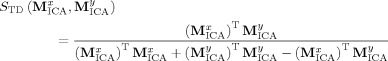
We can project Y back to the original data space to calculate the percentage of the variance in the original data for which the N ICA components account (Γ_ICA). We obtain

(4)

where pinv(W) denotes a pseudoinverse operation that can be implemented using a least‐squares optimization, and var(X) denotes a procedure for variance computation. One may compare the method described above to two other methods that have been proposed recently [Cordes and Nandy, 2006; Li et al., 2007] to estimate the optimal number of independent components that should be generated.

The Theory of PM

Measuring similarity in the spatial configuration of independent components

For simplicity, we define a family of independent components as referring either to (1) the set of all independent components for a single subject within a study of multiple subjects; or (2) the set of all independent components within a single scanning run in a study of a single individual, for whom multiple repeated scanning runs are obtained.

To measure the spatial similarity between two ICA components within differing families of components, we first convert each component into a Z‐score map. Letting IC _i denote the ith independent component and M ${}_{\mathit{\text{Z}}}^{\mathit{\text{i}}}$ denote its Z‐score map, we obtain

(5a)

where mean(·) and std(·) respectively denote the operations of computing the mean and the standard deviation across the entire 3D volume of components i. To obtain an ICA map, which represents a spatial pattern of significant functional activations or connectivity among brain regions, we threshold each Z‐score map of the component across the entire 3D volume. Let M ${}_{\text{ICA}}^{\text{i}}$ denote the ICA map of component i; Z _t denotes a given Z‐score threshold; and Z _U and Z _L denote the Z‐scores for the upper and lower bounds, corresponding to minimum tails of probability distribution of Z‐scores (usually, taking Z _L = − Z _U). We then obtain

(5b)

where x, y, and z denote spatial coordinates. We set Z _t = 2 (corresponding to a p‐value < 0.05), Z _U = 8, and Z _L = − 8 (both corresponding to sufficiently significant p‐values < 10⁻¹⁴). Each ICA map within one family reflects a unique spatial pattern for the corresponding independent component, because the spatial distributions of all components derived from this family are by definition maximally independent of one another—i.e., each of the components in a family contains minimal MI in their spatial distributions. Maps of two independent components, each drawn from differing families, however, may be uniquely similar to one another in that the ICA map from one family will likely find one and only one partner to which it is most similar from another family within the same study.

At least three robust indices are available to measure quantitatively the similarity in the spatial distributions of two ICA maps: the spatial correlation coefficient (SCC), MI [Pluim et al., 2003] and Tanimoto Distance (TD) [Chen and Reynolds, 2002]. Let M ${}_{\text{ICA}}^{\mathit{\text{x}}}$ and M ${}_{\text{ICA}}^{\mathit{\text{y}}}$ denote the two ICA maps of independent component x from family A and independent component y from family B, respectively; and let S _SCC, S _MI, and S _TD denote the measures of spatial similarity for M ${}_{\text{ICA}}^{\mathit{\text{x}}}$ with M ${}_{\text{ICA}}^{\mathit{\text{y}}}$ based on SCC, MI, and TD, respectively. We then define S _SCC, S _MI, and S _TD as follows:

Spatial correlation coefficient. We define S _SCC based on Pearson's correlation coefficient:

(6a)

where k = 1, 2, …, N denotes the order of voxels (after reshaping the 3D volume into a 1D volume), and N denotes the total number of voxels of M ${}_{\text{ICA}}^{\mathit{\text{x}}}$ and M ${}_{\text{ICA}}^{\mathit{\text{y}}}$.

Mutual information.

(6b)

where p (u, v) is the joint probability distribution function of M ${}_{\text{ICA}}^{\mathit{\text{x}}}$ and M ${}_{\text{ICA}}^{\mathit{\text{y}}}$, and p (u) and p (v) are the marginal probability distributions of M ${}_{\text{ICA}}^{\mathit{\text{x}}}$ and M ${}_{\text{ICA}}^{\mathit{\text{y}}}$, respectively. In practice, p (u, v) can be estimated approximately by the joint histogram of M ${}_{\text{ICA}}^{\mathit{\text{x}}}$ and M ${}_{\text{ICA}}^{\mathit{\text{y}}}$, and then p (u) and p (v) can be computed as p (u) = Σ_v p (u, v) and p (v) = Σ_u p (u, v).

Tanimoto distance.

(6c)

After applying SCC, MI, and TD to the two ICA maps, we converted the values of the similarity measures into Z‐scores to determine how significantly similar the two ICA maps are to one another: . We found that these three similarity indices performed comparably when applied within our PM algorithm (Fig. 1A).

Figure 1.

Comparing the performance of three measures of similarity: MI, TD, and spatial correlation. a: We used MI (panel a), TD (panel b), and SCC (panel c) to calculate normalized measurements of similarity (Z‐scores) between the ICA‐map of component 17 from Subject A, which served as the reference component (representing functional activity within the premotor area) and the ICA‐map of each of 50 independent components from Subject B. All three measures of similarity reached their peak value at component 11 from Subject B, thus indicating that component 11 from Subject B was maximally similar to component 17 from Subject A. The ICA‐maps of components 17 from Subject A (panel d) and 11 from Subject B (panel e) are indeed clearly similar visually. The peak z‐score and corresponding p‐value of this match was highly significant when evaluated with each of the three measures of similarity (for instance, with TD, Z _max = 5.83, p = 2.77 × 10⁻⁹). b: We also applied MI (panel a), TD (panel b), and SCC (panel c) to calculate normalized measurements of similarity (Z‐scores) between component 17 from Subject A, again used as the reference, and each of 50 components from Subject C. This time, the measurements of similarity differed. When using MI, component 6 from Subject C matched maximally with the reference (Z _max = 4.58, p = 2.32 × 10⁻⁶). However, when using either TD or SCC, component 4 from Subject C matched maximally with the reference (TD: Z _max = 6.27, p = 1.81 × 10⁻¹⁰; SCC: Z _max = 6.21, p = 2.56 × 10⁻¹⁰). The ICA‐maps of components 6 and 4 from Subject C are shown in panels (d) and (e), respectively. Note that component 4 is visually more similar to the reference component than is component 6; the latter actually represents functional activity within the primary motor area, rather than the premotor area. [Color figure can be viewed in the online issue, which is available at www.interscience.wiley.com.]

Although these similarity indices performed comparably when applied to data presented here, the accuracy of the indices may differ depending on the particular spatial configurations and datasets to which they are applied (Fig. 1B). These differences in accuracy merit further attention that is beyond the scope of this investigation. Here we will compute Z‐scores for all three similarity measures, SCC, MI, and TDD, and determine the matched component by majority rule—i.e., by selecting the component that is regarded as the best match by the majority of the three similarity measures (and if all differ, then by selecting the component that has the highest degree of significance among all three similarity measures in its match with the reference). We must emphasize, however, that the theory and implementation of our PM algorithm is independent of the use of any specific similarity measure, and therefore any of these three or other similarity measures may be used when employing PM.

Partner matching

Oveview. PM is a process of hierarchical clustering that identifies reproducible clusters of independent components. Each member component is consistently matched to all other components in the cluster based on a prespecified, statistically significant degree of spatial similarity. PM, however, differs from other conventional hierarchical clustering algorithms in two ways. First, PM constrains clustering so that any two independent components from the same family cannot be clustered together. Second, to achieve reproducible clusters, PM assesses retest reliability on every matched pair of independent components by performing bidirectional matching; instead of simply matching component IC_B from family B to component IC_A from family A using IC_A as a reference component, as is the case with most conventional hierarchical clustering algorithms, PM performs a further retesting procedure to assess whether component IC_A in turn matches component IC_B, using IC_B as the reference component. A cluster containing bidirectionally matched members is independent of the order of matching and thus is more reliable and robust than is a cluster that contains components matched in a single direction. PM bidirectionally matches every component to all other components in other families, thereby generating a closed set of clusters whose member components are all bidirectionally matched to a specified degree of average similarity.

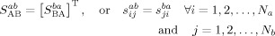
Let A and B denote any two different families of ICA components, let N_a and N_b denote the total number of components in families A and B, respectively, and let a_i and b_j denote the ith and jth respective components in families A and B, where i = 1, 2,…, N_a and j = 1,2, …, N_b. S(x,y) will denote a given similarity measure between components x and y. For PM, let p (1 ≤ p ≤ N_a) denote a given reference component in family A. We calculate the similarity between reference component a_p in family A and each of the components b_j for j = 1, 2, …, N_b in family B. We then find one component number u (1 ≤ u ≤ N_b) to make S(a_p, b_u) reach its maximum value, i.e., such that component b_u in family B has the largest similarity measure with component a_p in family A. The procedure to find component number u can be formulated as

This process achieves single‐directional matching. For bidirectional matching, we use b_u as a reference component to search for the most similar component in family A. Denoting this component number as q, it can be found by

Component a_p in family A and component b_u in family B are bidirectionally matched or, in our terminology, they are “Partner‐Matched” when and only when q = p.

Implementation of the PM procedure. PM entails the following computational steps:

Step 1: Compute and construct a similarity matrix for every two component families, A and B.

We compute a similarity measure and form a similarity matrix S _AB = {s_ij} ⊂ R ${}^{\mathit{\text{N}}{}_{\text{a}}\text{×}\mathit{\text{N}}{}_{\text{b}}}$ by

where S_m(·) denotes a similarity measure calculated using method m, e.g., using TD; a_i and b_j denote the ith and jth ICA component maps in families A and B, respectively.

Step 2: Identify single‐directional matches for each component in family A with all the components in family B.

First, we normalize into Z‐scores each row of the similarity matrix S _AB generated in Step 1 by subtracting the mean value and dividing by the standard deviation of the similarity measures.

We then determine the conditional PM matrix S ${}_{\text{AB}}^{\mathit{\text{a}}}$ = {s ${}_{\text{ij}}^{\text{a}}$} ⊂ R ${}^{\mathit{\text{N}}{}_{\text{a}}\text{×}\mathit{\text{N}}{}_{\text{b}}}$ using family A as a reference by

Thus, in matrix S ${}_{\text{AB}}^{\mathit{\text{a}}}$ = {s ${}_{\text{ij}}^{\text{a}}$} ⊂ R ${}^{\mathit{\text{N}}{}_{\text{a}}\text{×}\mathit{\text{N}}{}_{\text{b}}}$, each row of similarity measures contains at most only one nonzero value.

Step 3: Identify single‐directional matches for each component in family B with all the components in family A.

We first normalize each column of the similarity matrix S _AB generated in Step 1 into Z‐statistics by subtracting the mean value and dividing by the standard deviation of the similarity measures.

We then determine the conditional PM matrix S ${}_{\text{AB}}^{\mathit{\text{b}}}$ = {s ${}_{\text{ij}}^{\text{b}}$} ⊂ R ${}^{\mathit{\text{N}}{}_{\text{a}}\text{×}\mathit{\text{N}}{}_{\text{b}}}$ using family B as a reference by

Thus, in matrix S ${}_{\text{AB}}^{\mathit{\text{b}}}$ = {s ${}_{\text{ij}}^{\text{b}}$} ⊂ R ${}^{\mathit{\text{N}}{}_{\text{a}}\text{×}\mathit{\text{N}}{}_{\text{b}}}$, each column contains at most only one nonzero value.

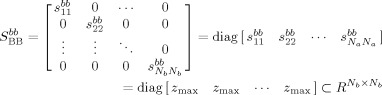
Step 4: Combine S ${}_{\text{AB}}^{\mathit{\text{a}}}$ with S ${}_{\text{AB}}^{\mathit{\text{b}}}$ to obtain a bidirectional matching matrix S ${}_{\text{AB}}^{\mathit{\text{ab}}}$ = {s ${}_{\text{ij}}^{\text{ab}}$} ⊂ R ${}^{\mathit{\text{N}}{}_{\text{a}}\text{×}\mathit{\text{N}}{}_{\text{b}}}$ by

where min{x,y} represents the operation of selecting the smaller of x and y.

We combine S ${}_{\text{AB}}^{\mathit{\text{a}}}$ with S ${}_{\text{AB}}^{\mathit{\text{b}}}$ by selecting the smaller of the two elements, s ${}_{\text{ij}}^{\text{a}}$ and s ${}_{\text{ij}}^{\text{b}}$, because s ${}_{\text{ij}}^{\text{a}}$ ≥ 0 and s ${}_{\text{ij}}^{\text{b}}$ ≥ 0; if s ${}_{\text{ij}}^{\text{ab}}$ > 0, s ${}_{\text{ij}}^{\text{a}}$ > 0, and s ${}_{\text{ij}}^{\text{b}}$ > 0 must exist, indicating that if we use a single component a_i in family A as a reference to search all N_b components {b_k |${}_{\mathit{\text{k}}\text{= 1, 2, …,}\mathit{\text{N}}{}_{\text{b}}}$} in family B, we will find a component b_j that has the largest similarity measure s ${}_{\text{ij}}^{\text{a}}$≥ z_ab; simultaneously, if we use a single component b_j in family B as a reference to search all N_a components {a _k |${}_{\mathit{\text{k}}\text{= 1, 2, …,}\mathit{\text{N}}{}_{\text{a}}}$} in family A, we will certainly find a component a_i that has the largest similarity measure s ${}_{\text{ij}}^{\text{b}}$ ≥ z_ab; and these two components will be similar to each other—i.e., they will be bidirectionally matched—to a degree that is at least s ${}_{\text{ij}}^{\text{ab}}$ = min { s ${}_{\text{ij}}^{\text{a}}$, s ${}_{\text{ij}}^{\text{b}}$} ≥ z_ab. On the other hand, if s ${}_{\text{ij}}^{\text{ab}}$ = 0, then either one or both s ${}_{\text{ij}}^{\text{a}}$ and s ${}_{\text{ij}}^{\text{b}}$ will be zero. In both of these cases, component a_i in family A and component b_j in family B will not be bidirectionally matched, and their degree of similarity will be zero.

Properties of the PM matrix. Based on the above description, we can easily infer the following properties of a PM matrix:

• i
  
• ii
  
• iii
  

Property (i) indicates that the PM matrix between any two families is independent of family order. With M families (M ≥ 2), the total number of PM matrices will be . Properties (ii) and (iii) are identical, either one indicating that components within the same family will be matched only with themselves to an infinite degree of similarity or to a predefined upper bound of the Z‐statistic, z _max.

Self‐Clustering Multiple Families of Independent Components

The PM theory just described establishes the principle that guides the automatic, bidirectional matching of independent components with a one‐to‐one spatial similarity across any two families of components. We then apply this theory to cluster multiple families of independent components repeatedly. Given M families, we assign a unique index number to each family using numbers 1, 2,…, M. For any family i ∈ {1, 2, …, M}, we use N(i) to denote the number of ICA components generated for family i. In PM, N(i) can be either the same or different for all families. We match every family with all other M − 1 families using our algorithm (Fig. 2a).

Figure 2.

First‐ and second‐level matching procedures: (a) First‐level matching procedure and (b) second‐level matching procedure (merging procedure).

Testing the rates of matching

The rate of first‐level matching. Let M denote the number of subjects in a group and N denote the number of components for each subject. After applying PM to the M subjects times, we obtain M root clusters. Each root cluster contains N_c subclusters (or simply “clusters”). Each cluster includes m (m ≤ M) components from m differing subjects in the group, where each component number is between 1 and N_c. The first‐level matching rate (FLMR), the matching rate between every pair of components in each cluster, is assessed using the smaller of the two PM Z‐scores or the larger of the two PM p‐values . In each cluster, only those components that have significant FLMRs (i.e., the maximum Z‐scores, Z _max, for the similarity of two components that are greater than a given Z‐threshold, or corresponding p‐values that are smaller than a prespecified p‐value) will be included for further processing and testing. Root clusters, clusters, and components can be represented using a tree‐like structure (Fig. 2b). The designated Z‐threshold could simply be determined empirically after studying several typical datasets. In the two datasets we used for demonstrating similarity measures (Fig. 1A,B) and in other datasets we have studied, for example, we have found that Z = 4.2 (corresponding to a p‐value of 2.67 × 10⁻⁵) would be a reasonable empirical threshold when 50 independent components were generated for each component family. Here, however, we propose a theoretical method to determine the Z‐threshold, which we call the Golden Section Method (GSM), after the well‐known golden section principle. This principle has been shown to be applicable for finding the optimal solution to many optimization problems, both in computer science [Lopez et al., 2002] and in signal and image processing [He et al., 2002; Xie et al., 2006].

GSM derives from a desire to optimize simultaneously both the sensitivity and specificity of the Z‐threshold in identifying similar components. Let N denote the total number of independent components generated for each component family (in our examples shown here, N = 50). A previously proposed maximum positive Z‐score is theoretically 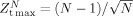[Shiffler, 1988]. If Z ${}_{\text{t}}^{\mathit{\text{N}}}$ denotes the Z‐score threshold we are seeking, then obviously Z ${}_{\text{t}}^{\mathit{\text{N}}}$ depends on Z ${}_{\text{t max}}^{\mathit{\text{N}}}$ and thus we could take a proportion of Z ${}_{\text{t max}}^{\mathit{\text{N}}}$ as Z ${}_{\text{t}}^{\mathit{\text{N}}}$, i.e., Z ${}_{\text{t}}^{\mathit{\text{N}}}$ = rZ ${}_{\text{t max′}}^{\mathit{\text{N}}}$, and r is a proportional ratio to be determined such that 0 < r < 1. As r increases, Z ${}_{\text{t}}^{\mathit{\text{N}}}$ increases, and thus the specificity of the binary classification between “matched” and “unmatched” also increases. However, as Z ${}_{\text{t}}^{\mathit{\text{N}}}$ increases, the sensitivity of the matching classification decreases. We can use Z ${}_{\text{t max}}^{\mathit{\text{N}}}$ − Z ${}_{\text{t}}^{\mathit{\text{N}}}$ to represent sensitivity and express it as a proportion of Z ${}_{\text{t}}^{\mathit{\text{N}}}$: Z ${}_{\text{t max}}^{\mathit{\text{N}}}$ − Z ${}_{\text{t}}^{\mathit{\text{N}}}$ = kZ ${}_{\text{t}}^{\mathit{\text{N}}}$ where 0 < k < ∞. As k increases, sensitivity also increases, whereas specificity decreases. To optimize this trade‐off of sensitivity with specificity, we can take k = r, in which case we will have r = Z ${}_{\text{t}}^{\mathit{\text{N}}}$/Z ${}_{\text{t max}}^{\mathit{\text{N}}}$ = (Z ${}_{\text{t max}}^{\mathit{\text{N}}}$ − Z ${}_{\text{t}}^{\mathit{\text{N}}}$)/Z ${}_{\text{t}}^{\mathit{\text{N}}}$, or r = (1 − r)/r, which can be rewritten as: r ² + r − 1 = 0. This yields a unique, positive‐value solution, , the well‐known Golden Section Ratio (GSR). Using this ratio, we obtain the desired Z‐score threshold based on the GSR: , where for an N = 50, Z ${}_{\text{t}}^{\text{50}}$ = 4.28.

The rate of second‐level matching. The FLMR evaluates only the degree of similarity between two components from two families and is therefore inadequate for evaluating the degree of overall similarity among all components within each cluster. This is because PM is independent of the order between each pair of group members but not necessarily between more than a pair of members. To evaluate the degree of overall similarity for an entire cluster, we must test for independence between all possible pairs of components across all group members. Let S_i denote the summation of all matching scores determined by the FLMR, where each matching score is binary––1 (matched) if the FLMR is larger than a given Z‐score threshold (we used the GSR‐determined threshold Z ${}_{\text{t}}^{\text{50}}$ = 4.28, corresponding to a p‐value of 1.87 × 10⁻⁵), and 0 (unmatched) otherwise. We define the second‐level matching rate (SLMR) as SLMR = S_i/M, where M is the total number of members in the group. The range of possible SLMR values is between 0 and 1. If SLMR is equal to 1, then the cluster achieves full PM, and the results of PM will be identical when matching any two group members, in any order. We then use the SLMR to evaluate the degree of similarity of each cluster. All clusters in each root cluster will be sorted in descending order based on their SLMR (i.e., decreasing SLMR).

Merging root clusters

All root clusters are first sorted in order of descending SLMR. The first root cluster having the highest SLMR of all root clusters is called a super cluster. Then, all other clusters are merged into this supercluster (Fig. 2b). Let M denote the total number of families, and N = Σ${}_{\mathit{\text{i}}\text{= 1}}^{\mathit{\text{M}}}$ N_i denote the total number of independent components generated for all the M families, where N_i denotes the number of components generated for the ith family. Calculate all PM similarity matrices for every two families and arrange them into one sparse square matrix S _PM such that S _PM = {s_ij} where 1 ≤ i ≤ N, 1 ≤ j ≤ N, and s_ij = 0 if components i and j are within the same family. The detailed merging process is described as follows:

• 1Set n = 0.
• 2Set n = n + 1.
• 3Check whether n > total number of ICA components N.
• 4If Yes, GOTO 18, otherwise continue with the following procedures.
• 5Search all matrix elements at the nth row of S _PM and include the indexes of all elements > 0 in a row vector u.
• 6Let p = [n u] (merging n and vector u).
• 7Sort p in an ascending order.
• 8Calculate the length of row vector p, Len_p. If Len_p < M, locate and fill those unmatched families within p with zeros.
• 9Calculate the length of row vector u, Len_u.
• 10Set m = 0.
• 11Set m = m + 1.
• 12Search all elements from S _PM at the u(m)th row (note: here m is the index of u) and include the indexes of all those elements < 0 in a row vector v.
• 13Merge u(m) and v and form a new vector q = [u(m) v].
• 14Sort q in an ascending order.
• 15Calculate the length of row vector q, Len_q. If Len_q < M, locate and fill those unmatched families within q with zeros.
• 16Update p by concatenating p with .
• 17Check whether m < Len_u. If yes, save p to a matrix P_n = p and then GOTO 2, otherwise GOTO 11.
• 18Calculate SLMR for every matrix P_n. If P_n has a square submatrix whose elements are all nonzero and column vectors are all the same, we call such a submatrix a Full PM Matrix (FPMM). Obviously, the greater the dimension of an FPMM of a P_n, the greater the SLMR of the P_n and thus the more reliable the cluster detected by the P_n. We sort all the detected clusters in descending order based on their SLMR and merge the clusters with same components into the cluster with greatest SLMR among these clusters.

Evaluating the reliability of clustering

Consistency of clusters. Because the SLMR reflects the degree of average similarity, equivalent to an average correlation coefficient among the independent components within each cluster, we can quantitatively estimate the reliability of each cluster by calculating the internal consistency index, Cronbach's Alpha (CA) [Carmines and Zeller, 1979], of each cluster using its SLMR. Let N denote the number of independent components in a given cluster c_i; CA can be calculated as:

(7)

Component reproducibility. CA estimates efficiently the reliability of each cluster based on the degree of similarity among independent components within the cluster. To evaluate further the reliability of the cluster, we also calculate the degree of component reproducibility within the cluster. Let n_i denote the number of components in the ith cluster. We use a χ² goodness‐of‐fit test to determine whether n_i components are significantly reproducible across the N group members. The significance of the p‐value of the χ ² test defines the reproducibility of the component within each cluster. This procedure can be described as follows:

• iConstruct a 2‐by‐2 contingency table: 
• ii
  Calculate the associated χ² statistic:

  

  where F(·) is a cumulative distribution function (CDF), Y ${}_{\text{1}}^{\text{u}}$ and Y ${}_{\text{1}}^{\text{l}}$ are the upper and lower limits of expected matched frequencies, and Y ${}_{\text{2}}^{\text{u}}$ and Y ${}_{\text{2}}^{\text{l}}$ are the upper and lower limits of expected unmatched frequencies.
• iiiCalculate the associated p‐value: We calculate a one‐tailed p‐value based on a χ² CDF with the degree of freedom (df) equal to 1 at value χ ².

Table  .

	Matched frequency	Unmatched frequency
Observed frequency	ni	N − ni
Expected frequency	E 1	E 2

Experimental Validations

We conducted three independent fMRI studies to validate the performance of our PM algorithm in detecting independent components that are reliable across subjects and across scanning runs within a single subject. In Study A, we scanned 13 healthy adults (8 men, 34.8 ± 15.2 years old; 5 women, 27.7 ± 6.7 years old) as they performed simple motor, visual, and auditory tasks. The order of these tasks was randomized across the 13 subjects. In Study B, we scanned a single subject (male, 18 years of age) with Tourette Syndrome (TS) [Cohen et al., 2001] as he performed a simple button‐pressing task over six scanning runs. All subjects were right‐handed, and subjects in Study A were free of previous neurological problems, psychiatric disorders, and head injury. The Columbia University Institutional Review Board approved the protocol, and all participants provided informed consent before the study.

Experimental paradigms

Study A: Auditory task. The auditory stimuli were programmed, delivered, and controlled using E‐Prime software (http://www.pstnet.com/products/e-prime). The stimuli were delivered via MRI‐compatible earphones (Resonance Technology). The auditory stimulus was an “alarm whistle” in Windows Pulse Code Modulation (PCM) format presented in mono with a sampling frequency of 11.025 kHz and a 16‐bit data precision. This stimulus was presented in a block‐design format with epochs of 20 s alternated with 20‐s epochs of silence with gaze fixation on a white cross‐hair located in the middle of a black background, over seven sound‐silence cycles.

Study A: Motor Task. The motor task was nearly identical in design and timing to that of the auditory task, except that the 20‐s epochs of task consisted of tapping the right index finger as quickly as possible in response to a cue displayed on the screen (a symbol changing from “+” to “×”).

Study A: Visual task. The visual task was similar in design to the auditory and motor tasks described above, with 20 s of visual stimulation. Stimuli were presented through fiber‐optic goggles (Resonance Technology). Visual stimulation was composed of a checkerboard that flashed at a frequency of 60 Hz and simultaneously rotated at a frequency of 0.5 Hz.

Study B: Button‐pressing task. This was conducted on one subject who pressed a button using his right hand at a time of his own selection, without presentation of any cue, on average every 25 s. The times when the subject pressed the button were recorded in LabView (National Instruments, http://www.ni.com/labview).

Image acquisition

In Study A, images were acquired on a GE 3T Signa Scanner (Milwaukee, WI). Head positioning in the magnet was standardized using the canthomeateal line. A T₁‐weighted sagittal localizing scan was used to position the axial images. In all subjects, a high‐resolution T₁‐weighted structural image with 34 axial slices (acquisition matrix: 256 × 256, FOV: 24 × 24 cm, slice thickness: 3.5 mm, contiguous) was positioned oriented parallel to the anterior commissure–posterior commissure (AC–PC) line. Functional images with 34 T₂‐weighted axial slices were acquired while subjects performed one of the three tasks (visual, motor, or auditory) described above, using a gradient‐recalled single‐shot echo‐planar pulse sequence with repetition time (TR) = 2200 ms, echo time (TE) = 60 ms, flip angle = 60°, acquisition matrix = 64 × 64, field of view (FOV) = 24 × 24 cm, slice thickness = 3.5 mm contiguous, in‐plane resolution was 3.75 × 3.75 mm, 128 images per experiment.

In Study B, imaging was performed using a GE 1.5T Signa Scanner (Milwaukee, WI). Parameters for the pulse sequence were TR = 1200 ms, TE = 60 ms, flip angle = 60°, acquisition matrix = 64 × 64, FOV = 20 × 20 cm, slice thickness = 8.6 mm, in‐plane resolution was 3.12 × 3.12 mm, 10 slices per imaging volume oriented parallel to the AC–PC line, 102 imaging volumes per run, and 6 runs for the entire study.

Image analysis

The entire image analysis procedure, including preprocessing, ICA, and the identification of independent components using PM, was performed using an integrated software package developed by the authors. In developing this software, we used a mixed‐language programming technique with C++ (for computation‐intensive procedures, such as the computation of similarity matrices), MATLAB (for user‐interface, ICA, and PM procedures), and JAVA (for 3D volume rendering of functional activation maps). This software also included all image preprocessing procedures running in a batch mode. These preprocessing procedures were implemented based on subroutines in two software packages, Statistical Parametric Mapping, Version 2 (SPM2) [http://www.fil.ion.ucl.ac.uk/spm/] and FMRIB Software Library (FSL) [http://www.fmrib.ox.ac.uk/fsl/]. We used subroutines in SPM2 to implement most of the image preprocessing procedures, including slice‐time correction, motion correction, spatial normalization, and spatial smoothing. Functional images were first corrected for timing differences between slices using a windowed Fourier interpolation to minimize their dependence on the reference slice [Jazzard et al., 2002]. Images were then motion‐corrected and realigned to the middle image of the middle scanning run. Images were discarded if the estimates for peak motion exceeded 1‐mm displacement or 2° rotation [Friston et al., 1996]. We used a subroutine within FSL, Brain Extraction Tool (BET) [Smith, 2002], to remove nonbrain tissue from the images. Next we filled the portions of the image that were previously occupied by nonbrain tissue with a special value, called NaN (not a number) so that the images remained the same size as the original images following brain extraction. Images were then spatially smoothed using a Gaussian‐kernel filter with a full width at half maximum (FWHM) of 8 mm. In all subsequent procedures, we converted the images into a smaller size that contained only non‐NaN values and an index table indicating the locations of all NaN values. The number of ICA components was estimated by using AIC–MDL criteria [Calhoun et al., 2001] and our variance analysis described in Eq. (4). The smoothed fMRI data from each subject and each run were then reduced from either 128 (Study A) or 102 (Study B) time points to 50 time points using PCA. ICA was then performed on the reduced 50 time‐point data for each subject or each run using the algorithm “Infomax” [Bell and Seinowski, 1995], with 1024 maximal ICA training steps and a unitary matrix as the initial weighting matrix. ICA generated 50 components for each dataset. Before running PM, two postprocessing procedures were performed on all ICA components. In the first procedure, all components were normalized to the T₁‐weighted Talairach template [Talairach and Tournoux, 1988] having a voxel size of 2 × 2 × 2 mm, thereby producing a normalized activation map with a standard matrix of 76 × 95 × 69 for each ICA component. Spatial normalization was performed for each subject as follows: (1) we coregistered the ICA components for a subject to the same subject's T₁‐weighted high‐resolution structural image using the first functional image of the subject as the source image; (2) we warped the T₁‐weighted structural image for the subject to the template and generated the respective deformation fields; (3) we then used these deformation fields to normalize all ICA components for this subject to the template,. An optional second postprocessing procedure, which we implemented for the purposes of data reduction and denoising, was based on a single‐level, two‐dimensional (2D), discrete wavelet transform (DWT) [Chang et al., 2000]. It was applied to all normalized ICA components using a well‐known 9/7‐tap biorthogonal wavelet [Lewis and Knowles, 1992]. Following the 2D DWT, each imaging slice of the normalized ICA component was decomposed into four subbands, labeled low–low (LL), low–high (LH), high–low (HL), and high–high (HH), each with a size of 38 × 48 voxels. The LL subband was a low‐frequency band representing the general (low‐frequency) spatial pattern of each ICA component. The other three subbands contained information representing primarily edges and noise for each component. We used the LL subband for each ICA component and thus reduced the size of each normalized ICA map from 79 × 95 × 69 voxels to 38 × 48 × 69 voxels, a size that permits faster computation of similarity matrices. We then used the matching, sorting, and merging procedures previously described (Experimental Validations section) to detect clusters of independent components that were significantly reproducible across subjects (Study A) or across runs for a single subject (Study B) based on the PM matrices.

RESULTS

Reproducibility Across Subjects Within a Group

After merging all root clusters into one super cluster, we evaluated the reproducibility of every cluster in each of the three experiments (auditory, motor, and visual) of Study A using CA, along with its associated χ² statistic and p‐value, as a measure of component reproducibility. We then sorted all CAs in descending order. We used the conventional threshold of CA ≥ 0.8 when evaluating the reliability [Carmines and Zeller, 1979] for the auditory, motor, and visual tasks, respectively (Fig. 3).

Figure 3.

Statistical tests for the degree of component matching. The panels in this figure show the statistical tests for each of the three tasks of Study A: (1) the SLMR, in purple, and (2) CA in red, both measures of the significance of the similarity between components, and (3) the p‐value associated with a χ² test of the significance of component reproducibility, in white. All three statistical tests were used to evaluate the degree of component matching for each root cluster within each task. We represented p‐values as 1 − p to allow values of all three similarity tests to be represented on a single scale ranging from 0 to 1, with 1 indicating greatest similarity. This figure shows the three test values for clusters in which CA ≥ 0.8: (a) auditory stimulation, (b) motor task, and (c) visual stimulation.

The most reliable clusters in each of the three tasks comprised 13 components, one from each subject. These three clusters likely represented neuronal activity within primary auditory, motor, and visual cortices during the performance of auditory, motor, and visual tasks, respectively (Figs. 4, 5, 6). Despite spatial variations in the components across subjects, PM clearly detected functional activations for each task in each subject. When we compared the 13 ICA maps (Figs. 4, 5, 6), we demonstrated that they were highly similar to one another across subjects and represented a significant fixed effect within the group (e.g., Fig. 7a).

Figure 4.

Reproducible components across subjects for auditory, motor, and visual tasks—Study A. These three figures show activation maps for each of the 13 subjects performing the three tasks in Study A: auditory (Fig. 4), motor (Fig. 5), and visual (Fig. 6). Each figure shows themost reproducible cluster. For each task, the most reliable cluster was detected in each of the 13 subjects, and it had the greatest spatial similarity across subjects (CA = 0.97, p = 0.00031 in Fig. 4; CA = 0.96, p = 0.00031 in Fig. 5; CA = 0.95, p = 0.00031 in Fig. 6). Each row represents a slice from the same location in the brain across the 13 subjects (Z‐level is the location of the slice in Talairach space). Each column depicts a single component across 10 slices within an individual subject.

Figure 5.

Reproducible components across subjects for auditory, motor, and visual tasks—Study A. These three figures show activation maps for each of the 13 subjects performing the three tasks in Study A: auditory (Fig. 4), motor (Fig. 5), and visual (Fig. 6). Each figure shows themost reproducible cluster. For each task, the most reliable cluster was detected in each of the 13 subjects, and it had the greatest spatial similarity across subjects (CA = 0.97, p = 0.00031 in Fig. 4; CA = 0.96, p = 0.00031 in Fig. 5; CA = 0.95, p = 0.00031 in Fig. 6). Each row represents a slice from the same location in the brain across the 13 subjects (Z‐level is the location of the slice in Talairach space). Each column depicts a single component across 10 slices within an individual subject.

Figure 6.

Reproducible components across subjects for auditory, motor, and visual tasks—Study A. These three figures show activation maps for each of the 13 subjects performing the three tasks in Study A: auditory (Fig. 4), motor (Fig. 5), and visual (Fig. 6). Each figure shows themost reproducible cluster. For each task, the most reliable cluster was detected in each of the 13 subjects, and it had the greatest spatial similarity across subjects (CA = 0.97, p = 0.00031 in Fig. 4; CA = 0.96, p = 0.00031 in Fig. 5; CA = 0.95, p = 0.00031 in Fig. 6). Each row represents a slice from the same location in the brain across the 13 subjects (Z‐level is the location of the slice in Talairach space). Each column depicts a single component across 10 slices within an individual subject.

Figure 7.

Averaged ICA‐maps of the five most reliable clusters and SPM‐map of 13 subjects from the auditory task—Study A. (a) and (b) respectively demonstrate the averaged ICA‐map of 13 components within Cluster 1 and averaged SPM‐map from the 13 subjects, all showing primary auditory activity; (c), (d), (e), and (f) show averaged ICA‐maps for Cluster 2 (CA = 0.95, p = 0.002), Cluster 3 (CA = 0.93, p = 0.002), Cluster 4 (CA = 0.92, p = 0.012) and Cluster 5 (CA = 0.87, p = 0.012), respectively, which reveal functional activity or connectivity within specific regions: (c) basal ganglia, (d) default‐mode network, including mesial prefrontal, posterior cingulate, and posterior temporal cortices, (e) inferior parietal (yellow arrow) and dorsolateral prefrontal (red arrow) cortices in the left cerebral hemisphere, (f) Inferior parietal (yellow arrow), and dorsolateral prefrontal (red arrow), and dorsal anterior cingulate (green arrow) cortices in the right hemisphere.

ICA in combination with PM also identified in each of the tasks components that were highly reproducible across subjects, located in brain regions that seemed to constitute functional neural systems that previously have been well described, and not obvious or trivial candidates for identification using hypothesis‐driven analytic strategies commonly identified using GLM‐based platforms. In fact, many of the time courses of the variation in fMRI signal within these components were not coupled tightly to the time courses of task cycling in these tasks, and activity in these neural systems would never be identified using those conventional platforms. A full report of the reproducible components identified in all these tasks is beyond the scope of this report. Nevertheless, we note that, after the component in primary auditory cortex, the four next‐most reliable components having CAs > 0.8 that were detected in the dataset for the auditory task included those representing functional activity within: (1) the basal ganglia (especially the lenticular) nuclei bilaterally (Fig. 7c, CA = 0.95, p = 0.002); (2) the so‐called “default‐mode” network [Greicius et al., 2003], which includes mesial prefrontal, posterior cingulate, and posterior temporal cortices (Fig. 7d, CA = 0.93, p = 0.002); (3) the dorsolateral prefrontal and inferior parietal cortices within the left hemisphere (Fig. 7e, CA = 0.92, p = 0.012); and (4) the dorsolateral prefrontal and inferior parietal cortices in the right hemisphere, together with the dorsal anterior cingulate cortex (Fig. 7f, CA = 0.87, p = 0.012).

The remarkable sensitivity of ICA in combination with PM in identifying reproducible activations across individuals within each stimulus modality stands in contrast to the activations identified using hypothesis‐driven, GLM‐based analyses that are most commonly employed, for example, within SPM [Friston et al., 1995]. We analyzed these same fMRI datasets with SPM2 (http://www.fil.ion.ucl.ac.uk/spm/software/spm2), using all default parameters, without high‐pass filtering. For each subject, we generated a block‐design matrix with two conditions, “stimulus off” and “stimulus on”, based on the timing and duration of the cycling of the task stimuli. We then produced a t‐contrast (ON vs. OFF) map, imposed a p‐threshold ≤ 0.001 (uncorrected for multiple comparisons), converted each t‐map to a Z‐score map, and averaged the Z‐maps across all 13 subjects to yield a group‐average Z‐map (e.g. Fig. 7b). The group maps generated by ICA–PM and SPM both detected activity in the same primary sensory or motor cortex, but the average group effects detected by SPM were clearly less significant than those detected by ICA–PM (e.g., Fig. 7a,b).

We examined within each subject the time courses of signal variation for these components in relation to the time course of the hypothesized neuronal response to the task (which was obtained by convolving the times of task cycling with the canonical hemodynamic response function (HRF), and which together we term simply “the hypothesized HRF”). We correlated the ICA time course with the hypothesized HRF for all 50 components from each subject. Statistically significant correlation coefficients indicated some degree of phase‐locking of the time course of the component with the hypothesized HRF. The time courses of the components, however, generally were not tightly coupled with the hypothesized HRF for any reproducible component, including those representing activity in the primary sensory or motor cortices, where the greatest correlation with the hypothesized HRF would be expected (Figs. 8 and 9). The relatively poor phase‐locking of the time course of these components with the hypothesized HRF likely accounts for the relatively poor sensitivity of the hypothesis‐driven, GLM‐based analyses within SPM to detect activity in these regions compared with that of ICA–PM.

Figure 8.

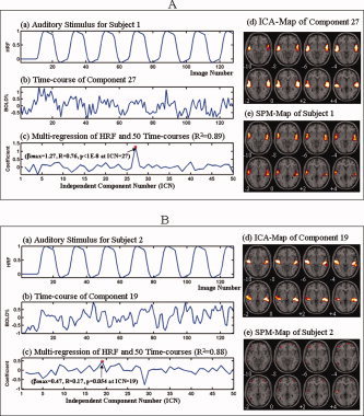
Comparing ICA–PM and SPM when detecting auditory processing in four subjects—Study A. These figures shows the hypothesized HRF derived from the auditory task in Panel (a); the blood oxygen level dependent (BOLD) response to the task measured by the time‐course of the component identified by PM in Panel (b); the temporal similarity between the HRF and the component time courses measured by multiregression and correlation in Panel (c); the ICA‐map of the PM‐identified component in Panel (d); and the SPM‐map of each of the 4 subjects in Panel (e). We conducted multiregression analysis on the HRF and the timecourses of all 50 components for each subject. We denoted as β_max or β_PM the regression coefficients of the component whose time course correlated most strongly with that of the hypothesized HRF, and of the component identified by PM, respectively. We also computed the Pearson correlation coefficient R and pvalue between the HRF and the time‐course of the PM‐identified component. Because we compared these values across 50 components for each subject, we used a corrected p‐value threshold = 0.05/50 = 0.001 to assess whether the temporal correlation was statistically significant. 8A: Both the ICA‐map of component 27 in this subject and the SPM‐map could clearly detect activity associated with the auditory processing in this task. The correlation of the time‐course of this component with the hypothesized HRF is the greatest of all such correlations calculated for all 50 components generated for this subject (β_PM = β_max = 1.27, R = 0.76, p < 10⁻⁸), indicating that the time course of this component is correlated, or phase‐locked, with the hypothesized HRF. 8B: PM clearly detected auditory activity (component 19) in Subject 1. SPM, however, detected this same auditory activity only weakly, and the SPM map is contaminated either by noise or by interference from other neuronal activity in these regions. The time course of component 19 correlated most strongly with the hypothesized time course among all 50 of the ICA‐generated components, but not significantly (β_PM = β_max = 0.47, R = 0.17, p = 0.054), indicating that it was not tightly phase‐locked to the hypothesized HRF. 9A, 9B: Similarly, PM detected auditory activity in component 15 of Subject 3 and component 3 of Subject 4, whereas SPM did not. The correlations of the time courses of these components with the hypothesized HRF, however, were neither strongest among all 50 ICA‐generated components nor significant in these subjects (β_PM = 0.19 at component 15 <β_max = 0.49 at component 39, R = 0.018, p = 0.84 in Subject 3; β_PM= 0.33 at component 3 <β_max = 0.47 at component 31, R = 0.013, p = 0.89 in Subject 4), indicating that these components are not temporally tightly phase‐locked with the hypothesized HRF. This absence of significant phase‐locking likely accounts for the failure of SPM‐based analyses to detect auditory activation in these subjects (panel e in each figure). [Color figure can be viewed in the online issue, which is available at www.interscience.wiley.com.]

Figure 9.

Comparing ICA–PM and SPM when detecting auditory processing in four subjects—Study A. These figures shows the hypothesized HRF derived from the auditory task in Panel (a); the blood oxygen level dependent (BOLD) response to the task measured by the time‐course of the component identified by PM in Panel (b); the temporal similarity between the HRF and the component time courses measured by multiregression and correlation in Panel (c); the ICA‐map of the PM‐identified component in Panel (d); and the SPM‐map of each of the 4 subjects in Panel (e). We conducted multiregression analysis on the HRF and the timecourses of all 50 components for each subject. We denoted as β_max or β_PM the regression coefficients of the component whose time course correlated most strongly with that of the hypothesized HRF, and of the component identified by PM, respectively. We also computed the Pearson correlation coefficient R and pvalue between the HRF and the time‐course of the PM‐identified component. Because we compared these values across 50 components for each subject, we used a corrected p‐value threshold = 0.05/50 = 0.001 to assess whether the temporal correlation was statistically significant. 8A: Both the ICA‐map of component 27 in this subject and the SPM‐map could clearly detect activity associated with the auditory processing in this task. The correlation of the time‐course of this component with the hypothesized HRF is the greatest of all such correlations calculated for all 50 components generated for this subject (β_PM = β_max = 1.27, R = 0.76, p < 10⁻⁸), indicating that the time course of this component is correlated, or phase‐locked, with the hypothesized HRF. 8B: PM clearly detected auditory activity (component 19) in Subject 1. SPM, however, detected this same auditory activity only weakly, and the SPM map is contaminated either by noise or by interference from other neuronal activity in these regions. The time course of component 19 correlated most strongly with the hypothesized time course among all 50 of the ICA‐generated components, but not significantly (β_PM = β_max = 0.47, R = 0.17, p = 0.054), indicating that it was not tightly phase‐locked to the hypothesized HRF. 9A, 9B: Similarly, PM detected auditory activity in component 15 of Subject 3 and component 3 of Subject 4, whereas SPM did not. The correlations of the time courses of these components with the hypothesized HRF, however, were neither strongest among all 50 ICA‐generated components nor significant in these subjects (β_PM = 0.19 at component 15 <β_max = 0.49 at component 39, R = 0.018, p = 0.84 in Subject 3; β_PM= 0.33 at component 3 <β_max = 0.47 at component 31, R = 0.013, p = 0.89 in Subject 4), indicating that these components are not temporally tightly phase‐locked with the hypothesized HRF. This absence of significant phase‐locking likely accounts for the failure of SPM‐based analyses to detect auditory activation in these subjects (panel e in each figure). [Color figure can be viewed in the online issue, which is available at www.interscience.wiley.com.]

Reproducibility Across Multiple Scanning Runs in a Single Subject

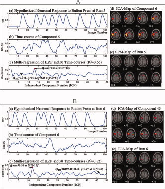
We identified three significantly reproducible clusters of components (CA > 0.8, p < 0.02) in the button‐pressing task of Study B. PM identified activity in the primary motor (M1) and supplementary motor (SMA) cortices within Cluster 1 (CA = 0.91, p = 0.01) across all 6 runs. In contrast, SPM2 run with all default parameters detected task‐related activity in these regions only on the third run, because only in this run did the time course of the hypothesized HRF for the task correspond well with the HRF actually generated by the task, as reflected in the time course for this component (Figs. 10, 11, 12). PM also identified reproducible Cluster 2 (CA = 0.87, p = 0.01) and Cluster 3 (CA = 0.85, p = 0.01) of independent components in which the HRFs correlated poorly with the hypothesized HRF for the task and that presumably represent higher‐level cognitive activity associated with the motor task. These components included one (within Cluster 2) located in dorsolateral prefrontal and parietal cortices in the left hemisphere together with the superior frontal gyrus (Fig. 13), and another (within Cluster 3) in the premotor cortex bilaterally (Fig. 14).

Figure 10.

Comparison of ICA‐PM and SPM in detecting primary motor activity in a single subject within six scanning runs—Study B. These figures show the hypothesized HRF associated with the intermittent, self‐cued button‐pressing task for each run in Panel (a); the BOLD response to the task in Panel (b); the multiregression and correlation between the HRF and the component time courses in Panel (c); the ICA‐map of the PM‐identified component in Panel (d); and the SPM‐map of each run in Panel (e). PM clearly detected motor activity within primary motor cortex (M1) and SMA in each of the 6 runs. SPM, however, detected similar activity in M1 and SMA only in Run 3 (Fig. 11a). SPM detected M1 motor activity very weakly in Runs 2 (Fig. 10b) and 5 (Fig. 12a), but failed to detect it entirely in Runs 1 (Fig. 10a), 4 (Fig. 11b), and 6 (Fig. 12b). The analyses of multiregression and correlation showed that only in Run 3 was the neuronal response during the task maximally similar to and significantly correlated in time with the HRF (β_PM = β_max = 0.18, R = 0.39, p < 0.0001). In all other runs, it was neither maximally similar to, nor significantly correlated with, the hypothesized HRF (β_PM = −0.041 < β_max = 0.12, R = 0.14, p = 0.17 in Run 1; β_PM = 0.017 < β_max = 0.12, R = 0.059, p = 0.55 in Run 2; β_PM = −0.26 < β_max = 0.20, R = 0.086, p = 0.39 in Run 4; β_PM = 0.041< β_max = 0.26, R = 0.12, p = 0.25 in Run 5; β_PM = 0.069 < β_max = 0.30, R = −0.11, p = 0.27 in Run 6). [Color figure can be viewed in the online issue, which is available at www.interscience.wiley.com.]

Figure 11.

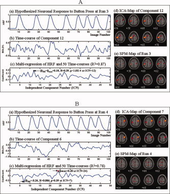
Comparison of ICA‐PM and SPM in detecting primary motor activity in a single subject within six scanning runs—Study B. These figures show the hypothesized HRF associated with the intermittent, self‐cued button‐pressing task for each run in Panel (a); the BOLD response to the task in Panel (b); the multiregression and correlation between the HRF and the component time courses in Panel (c); the ICA‐map of the PM‐identified component in Panel (d); and the SPM‐map of each run in Panel (e). PM clearly detected motor activity within primary motor cortex (M1) and SMA in each of the 6 runs. SPM, however, detected similar activity in M1 and SMA only in Run 3 (Fig. 11a). SPM detected M1 motor activity very weakly in Runs 2 (Fig. 10b) and 5 (Fig. 12a), but failed to detect it entirely in Runs 1 (Fig. 10a), 4 (Fig. 11b), and 6 (Fig. 12b). The analyses of multiregression and correlation showed that only in Run 3 was the neuronal response during the task maximally similar to and significantly correlated in time with the HRF (β_PM = β_max = 0.18, R = 0.39, p < 0.0001). In all other runs, it was neither maximally similar to, nor significantly correlated with, the hypothesized HRF (β_PM = −0.041 < β_max = 0.12, R = 0.14, p = 0.17 in Run 1; β_PM = 0.017 < β_max = 0.12, R = 0.059, p = 0.55 in Run 2; β_PM = −0.26 < β_max = 0.20, R = 0.086, p = 0.39 in Run 4; β_PM = 0.041< β_max = 0.26, R = 0.12, p = 0.25 in Run 5; β_PM = 0.069 < β_max = 0.30, R = −0.11, p = 0.27 in Run 6). [Color figure can be viewed in the online issue, which is available at www.interscience.wiley.com.]

Figure 12.

Comparison of ICA‐PM and SPM in detecting primary motor activity in a single subject within six scanning runs—Study B. These figures show the hypothesized HRF associated with the intermittent, self‐cued button‐pressing task for each run in Panel (a); the BOLD response to the task in Panel (b); the multiregression and correlation between the HRF and the component time courses in Panel (c); the ICA‐map of the PM‐identified component in Panel (d); and the SPM‐map of each run in Panel (e). PM clearly detected motor activity within primary motor cortex (M1) and SMA in each of the 6 runs. SPM, however, detected similar activity in M1 and SMA only in Run 3 (Fig. 11a). SPM detected M1 motor activity very weakly in Runs 2 (Fig. 10b) and 5 (Fig. 12a), but failed to detect it entirely in Runs 1 (Fig. 10a), 4 (Fig. 11b), and 6 (Fig. 12b). The analyses of multiregression and correlation showed that only in Run 3 was the neuronal response during the task maximally similar to and significantly correlated in time with the HRF (β_PM = β_max = 0.18, R = 0.39, p < 0.0001). In all other runs, it was neither maximally similar to, nor significantly correlated with, the hypothesized HRF (β_PM = −0.041 < β_max = 0.12, R = 0.14, p = 0.17 in Run 1; β_PM = 0.017 < β_max = 0.12, R = 0.059, p = 0.55 in Run 2; β_PM = −0.26 < β_max = 0.20, R = 0.086, p = 0.39 in Run 4; β_PM = 0.041< β_max = 0.26, R = 0.12, p = 0.25 in Run 5; β_PM = 0.069 < β_max = 0.30, R = −0.11, p = 0.27 in Run 6). [Color figure can be viewed in the online issue, which is available at www.interscience.wiley.com.]

Figure 13.

ICA‐maps and corresponding time courses of reproducible component clusters 2 & 3 from a single subject with six scanning runs—Study B. These figures are both divided into six panels, one each for Runs 1–6. Each panel provides for the specific component in that run that is a member of the reproducible cluster across runs: (a) the hypothesized HRF, (b) the time course in the identified component, and (c) the ICA‐map. The ICA‐maps are highly similar to one another across runs. The maps in Figure 13 represent functional activity within posterior parietal cortex and parietal prefrontal cortex. The maps in Figure 14 represent activity in the premotor area bilaterally. Because none of the components shown in Figures 13 and 14 are the components at which the multiregressions reach bmax, none of the component time courses are temporally tightly phase‐locked to the HRF. Figure 13 – Run1: R = 0.11, p = 0.28; Run 2: R = −0.11, p = 0.29; Run 3 R = −0.050, p = 0.61; Run 4: R = 0.067, p = 0.50; Run 5: R = −0.15, p = 0.13; Run 6: R = −0.11, p = 0.26. Figure 14 – Run 1: R = 0.12, p = 0.22; Run 2: R = 0.04, p = 0.69; Run 3: R = −0.12, p = 0.24; Run 4: R = 0.097, p = 0.33; Run 5: R = 0.16, p = 0.10; Run 6: R = −0.19, p = 0.047. [Color figure can be viewed in the online issue, which is available at www.interscience.wiley.com.]

Figure 14.

ICA‐maps and corresponding time courses of reproducible component clusters 2 & 3 from a single subject with six scanning runs—Study B. These figures are both divided into six panels, one each for Runs 1–6. Each panel provides for the specific component in that run that is a member of the reproducible cluster across runs: (a) the hypothesized HRF, (b) the time course in the identified component, and (c) the ICA‐map. The ICA‐maps are highly similar to one another across runs. The maps in Figure 13 represent functional activity within posterior parietal cortex and parietal prefrontal cortex. The maps in Figure 14 represent activity in the premotor area bilaterally. Because none of the components shown in Figures 13 and 14 are the components at which the multiregressions reach bmax, none of the component time courses are temporally tightly phase‐locked to the HRF. Figure 13 – Run1: R = 0.11, p = 0.28; Run 2: R = −0.11, p = 0.29; Run 3 R = −0.050, p = 0.61; Run 4: R = 0.067, p = 0.50; Run 5: R = −0.15, p = 0.13; Run 6: R = −0.11, p = 0.26. Figure 14 – Run 1: R = 0.12, p = 0.22; Run 2: R = 0.04, p = 0.69; Run 3: R = −0.12, p = 0.24; Run 4: R = 0.097, p = 0.33; Run 5: R = 0.16, p = 0.10; Run 6: R = −0.19, p = 0.047. [Color figure can be viewed in the online issue, which is available at www.interscience.wiley.com.]

DISCUSSION

We tested the effectiveness of our PM algorithm to identify reproducible independent components automatically in fMRI time series by applying it first to the analysis of fMRI data in a study of 13 healthy subjects performing simple auditory, motor, and visual tasks (Study A). PM accurately identified clusters of highly reproducible components across subjects in each of the stimulus modalities. The first most reproducible cluster identified in each experiment represented functional activity in the primary sensory or motor cortices that subserve these tasks. PM automatically identified 10 component clusters in the auditory task, 9 in the motor, and 10 in the visual task that were highly reproducible, as attested by CA values > 0.8. The most reliable cluster from each experiment was maximally reproducible, in that the PM cluster identified the same component in all 13 subjects. Moreover, that cluster showed the highest degree of consistency in spatial similarity across subjects (CA > 0.9) for all the identified component clusters. ICA–PM demonstrated substantially greater sensitivity in detecting activity in these primary sensory and motor cortices than did the hypothesis‐driven, GLM‐based analyses within SPM, likely because the time courses of fMRI signal variation in the components generally were not tightly coupled with the HRF hypothesized for the known time courses of task stimuli for any of the reproducible components, including those representing activity in the primary sensory or motor cortices. The maximal reproducibility of the components in these clusters, the highly significant similarity in their spatial configuration, and their location in precisely the same sensory or motor cortices known to subserve these tasks together demonstrate that these components identified by PM have excellent face validity and that they likely do indeed represent neuronal activity induced by each of the three tasks.

In addition to identifying the components in primary sensory or motor cortices, where the time‐course of activity correlated significantly with the time‐course of these auditory, motor, and visual tasks, our PM algorithm also identified reliable independent components that represent nontask related neural activity in cortical and subcortical regions, where the time course of the component did not correlate closely with the time course of the task, and where SPM was unable to detect those nontask‐related activities using a general linear model. For example, in the auditory task we identified four reliable clusters in addition to the component representing activity in primary auditory cortex. These components represented activity (1) in basal ganglia nuclei, (2) in so‐called “default‐mode” networks, (3) in prefrontal and parietal cortices of the left hemisphere, and (4) in prefrontal and parietal cortices of the right hemisphere.

Moreover, in a single subject performing an intermittent button‐pressing task over six scanning runs, our algorithm detected three highly reproducible independent components, representing functional activation in (1) primary motor cortices, (2) dorsolateral prefrontal and parietal cortices in the left hemisphere, and in the superior frontal gyrus, and (3) premotor cortex bilaterally. Our algorithm detected these components each of the six runs with this subject despite interference from neuronal activity caused by the occurrence of motor tics associated with TS. PM even detected task‐driven activations when the time courses of the actual neuronal responses to the task were not phase‐locked with the hypothesized HRF. Once again, an SPM‐based analysis of these datasets failed to detect these activations, and again the HRF actually generated by the task correlated poorly with the hypothesized HRF. Thus, PM can identify reliable components even when the primary neuronal activity is not phase‐locked with the tasks or when interference from other neural activity is present, because PM detects those components based on the reproducibility and similarity of a spatial pattern of temporal activity, not based on the hypothesized HRF.

Reproducible components identified by PM represent not only task‐induced activations, but activations of brain regions that compose an independent, “functionally connected” neural system. By definition, independent components identified through application of spatial ICA to an fMRI dataset must have the following spatial and temporal characteristics: (1) the nongaussianity in spatial distribution of gray‐scale values must be maximized within each component and (2) the MI of time courses must be maximized within and minimized between components. The maximized nongaussianity of the spatial distribution of gray‐scale values in independent components ensures that only a small number of voxels have significantly higher gray‐scale values (surpassing a specified threshold) than do the remaining numerous voxels within that distribution. Thus, the components represent a configuration of voxels across space that have a particular hemodynamic response during performance of a particular task [Esposito et al., 2005]. This spatial configuration, however, also represents the voxels in distinct brain regions that are presumed to be “functionally connected,” in that the time courses of those voxels are maximally phase‐coupled and coherent [Esposito et al., 2005]. In contrast, conventional methods for voxel‐wise analyses of fMRI time series, such as those based on GLM within SPM, are univariate methods and thus are inherently unable to reveal spatiotemporal relationships between voxels and their degree of functional connectivity [Friston et al., 1993; McKeown et al., 1998; McKeown and Sejnowski, 1998; van de Ven et al., 2004].

Consistent with these inherent differences in the analysis of fMRI data using PM–ICA and SPM, the activation maps for one cluster identified by PM–ICA in the button‐pressing task in Study B show not only clear activation within the primary motor cortex, but also activation within the supplementary motor area (Figs. 10, 11, 12). These maps and findings suggest that the primary and supplementary motor cortices are functionally connected, in accord with the known neurophysiology and anatomical connectivity of these regions in the human brain [Frackowiak et al., 2004]. The corresponding activation maps generated by SPM, however, do not show clear activation of the supplementary motor area and therefore do not provide evidence that it coactivates or is functionally connected with primary motor cortices.

As shown here and elsewhere, PM can also identify reproducible components whose time courses are not tightly phase‐locked with a task. These components may reflect patterns of genuine neural activity that are generated by higher‐level cognitive processes that the task engages. In our experiment of a single subject pressing a button intermittently across multiple scanning runs, for example, the time courses of Clusters 2 and 3, which represented activations located in dorsolateral prefrontal and parietal cortices in the left hemisphere, and in the superior frontal gyrus and premotor cortex bilaterally, were much less phase‐locked with the timing of the button press than was the time course for Cluster 1, which represented activation in primary and supplementary motor cortices. Perhaps Clusters 2 and 3 represented activity in the regions that are involved in higher‐level planning of the button press, rather than in the lower‐level execution of motor commands within motor cortex. Hypothesis‐driven methods for detecting task‐related brain activity, such as voxel‐wise analyses using GLM, may fail to detect such components because they presume a high correlation and tight phase‐locking of the hypothesized hemodynamic response with the time course of neuronal activity.

PM also makes possible the statistical comparison of ICA components across differing groups of subjects. ICA components generated from differing subjects and groups of subjects cannot be compared directly because ICA alone does not identify which of the many independent components generated by ICA algorithms represent the same neuronal activity across groups. PM, however, helps to identify the components that likely do represent the same neuronal (or nonneuronal) activity across subjects, and it does so automatically by clustering together those components that are significantly similar in their spatial and temporal patterns of activation, regardless of the order in which those components were originally generated by ICA. Analysis of the time courses of activity in the identified clusters can then help to determine which clusters likely represent neuronally derived signal that is either tightly or loosely time‐locked with the task. Moreover, the use of rigorous, quantitative constraints on similarity (e.g., CA > 0.8 and p < 0.05) ensures the reproducibility of clusters to a prespecified degree of statistical confidence.

Another potentially useful feature of PM is that it can be used to detect patterns of activation that are unique to an individual subject within a group of subjects—i.e., patterns that are reliable across scanning runs for that subject but that are not reproducible across other subjects of the group. PM can thus identify, for example, unique variations in task‐related cognitive strategies within the group that would not be detectable when only analyzing across members of the group. Therefore, the study of individual differences in cognitive strategies, as they are represented in the spatial and temporal patterns of neural activity generated by performing a task, now seems possible.

Our findings demonstrate clearly that the automated identification of robustly reproducible, independent components—a necessary, though not sufficient, condition for the determination of their validity—is possible using our PM algorithm. By identifying reproducible components automatically, PM will make feasible the analysis of large‐sample fMRI datasets that generate enormous numbers of components. Moreover, the most reproducible components identified by PM in group studies will likely represent neuronally derived signal within functionally connected neural systems, particularly if the additional constraint is imposed that the average time course of the reproducible component is at least loosely time‐locked to the time course of the task. The vast number of components involved and their spatial variability across individuals would otherwise render impossible the objective and accurate identification of corresponding components across individuals using visual inspection alone.

In conclusion, compared with more conventional, hypothesis‐driven methods for the analysis of fMRI datasets, ICA offers considerable advantages for the detection of neuronally derived and task‐related signal. ICA generates components that can be used to study functional connectivity, to detect nonphase‐locked functional activations, and to reduce noise in fMRI datasets. These advantages cannot be realized, however, without a means of identifying automatically and accurately the relatively small number of reliable components from among the enormous number of components that are generated within and across individuals in large‐sample studies. PM thus helps to make available to investigators the many potential uses of ICA, and it will thereby significantly facilitate the practical application of ICA to the analysis of fMRI datasets when exploring neuronal activity and functional connectivity in differing brain regions, and when trying to reduce noise in fMRI datasets, both within and between large groups of subjects, and within single individuals studied across time.

REFERENCES

- Akaike H ( 1974): A new look at statistical model identification. IEEE Trans Automatic Control 19: 716–723. [Google Scholar]
- Amari S ( 1998): Neural gradient works efficiently in learning. Neural Comput 10: 251–276. [Google Scholar]
- Bell AJ,Sejnowski TJ ( 1995): An information‐maximization approach to blind separation and blind deconvolution. Neural Comput 7: 1129–1159. [DOI] [PubMed] [Google Scholar]
- Biswal BB,Ulmer JL ( 1999): Blind source separation of multiple signal sources of fMRI data sets using independent component analysis. J Comput Assist Tomogr 23: 265–271. [DOI] [PubMed] [Google Scholar]
- Calhoun VD,Adali T,Pearlson GD,Pekar JJ ( 2001): A method for making group inferences from functional MRI data using independent component analysis. Hum Brain Mapp 14: 140–151. [DOI] [PMC free article] [PubMed] [Google Scholar]
- Cardoso JF,Laheld BH ( 1996): Equivariant adaptive source separation. IEEE Trans Signal Process 44: 3017–3030. [Google Scholar]
- Cardoso JF,Souloumiac A ( 1993): Blind beamforming for non‐Gaussian signals. IEE Proc 140: 362–370. [Google Scholar]
- Carmines EG,Zeller RA ( 1979): Reliability and Validity Assessment. Newbury Park: Sage Publications. [Google Scholar]
- Chang SG,Yu B,Vetterli M ( 2000): Adaptive wavelet thresholding for image denoising and compression. IEEE Trans Image Process 9: 1532–1546. [DOI] [PubMed] [Google Scholar]
- Chen X,Reynolds CH ( 2002): Performance of similarity measures in 2D fragment‐based similarity searching: Comparison of structural descriptors and similarity coefficients. J Chem Inf Comput Sci 42: 1407–1414. [DOI] [PubMed] [Google Scholar]
- Cohen DJ,Jankovic J,Goetz CG ( 2001): Tourette Syndrome. Philadelphia: Lippincott Williams & Wilkins. [Google Scholar]
- Comon P ( 1994): Independent component analysis—A new concept? Signal Process 36: 287–314. [Google Scholar]
- Cordes D,Nandy RR ( 2006): Estimation of the intrinsic dimensionality of fMRI data. NeuroImage 29: 145–154. [DOI] [PubMed] [Google Scholar]
- Esposito F,Formisano E,Seifritz E,Goebel R,Morrone R,Tedeschi G,Di Salle F ( 2002): Spatial independent component analysis of functional MRI time‐series: To what extent do results depend on the algorithm used? Hum Brain Mapp 16: 146–157. [DOI] [PMC free article] [PubMed] [Google Scholar]
- Esposito F,Scarabino T,Hyvarinen A,Himberg J,Formisano E,Comani S,Tedeshi G,Goebel R,Seifritz E,Salle FD ( 2005): Independent component analysis of fMRI group studies by self‐organizing clustering. Neuroimage 25: 193–205. [DOI] [PubMed] [Google Scholar]
- Formisano E,Goebel R ( 2003): Tracking cognitive processes with functional MRI mental chronometry. Curr Opin Neurobiol 13: 174–181. [DOI] [PubMed] [Google Scholar]
- Frackowiak RSJ,Friston KJ,Frith CD,Dolan RJ,Price CJ,Zeki S,Ashburner J,Penny W ( 2004): Human Brain Function, 2nd ed. San Diego: Elsevier Science. [Google Scholar]
- Friston KJ,Frith CD,Liddle PF,Frackowiak RS ( 1993): Functional connectivity: The principle‐component analysis of large (PET) data sets. J Cereb Blood Flow Metab 13: 5–14. [DOI] [PubMed] [Google Scholar]
- Friston KJ,Holmes AP,Worsley KJ,Poline JP,Fritch CD,Frackowiak RSJ ( 1995): Statistical parametric maps in functional imaging: A general linear model. Hum Brain Mapp 2: 189–210. [Google Scholar]
- Friston KJ,Williams S,Howard R,Frackowiak RS,Turner R ( 1996): Movement‐related effects in fMRI time‐series. Magn Reson Med 35: 346–355. [DOI] [PubMed] [Google Scholar]
- Friston KJ,Josephs O,Zarahn E,Holmes AP,Rouquette S,Poline JB ( 2000): To smooth or not smooth?—Bias and efficiency in fMRI time‐series analysis. Neuroimage 12: 196–208. [DOI] [PubMed] [Google Scholar]
- Greicius MD,Krasnow B,Reiss AL,Menon V ( 2003): Functional connectivity in the resting brain: A network analysis of the default mode hypothesis. Proc Natl Acad Sci USA 1: 253–258. [DOI] [PMC free article] [PubMed] [Google Scholar]
- Gusnard DA,Raichle ME ( 2001): Searching for a baseline: Functional imaging and the resting human brain. Nat Rev Neurosci 2: 685–694. [DOI] [PubMed] [Google Scholar]
- He C,Zheng YF,Ahalt SC ( 2002): Object tracking using the Gabor wavelet transform and the golden section algorithm. IEEE Trans Multimedia 4: 528–538. [Google Scholar]
- Huettel SA,Song AW,McCarthy G ( 2004): Functional Magnetic Resonance Imaging. Sunderland: Sinauer Associates. [Google Scholar]
- Himberg J,Hyvarinen A,Esposito F ( 2004): Validating the independent components of neuroimaging time series via clustering and visualization. NeuroImage 22: 1214–1222. [DOI] [PubMed] [Google Scholar]
- Hyvärinen A ( 1999a): Fast robust fixed‐point algorithms for independent component analysis. IEEE Trans Neural Netw 10: 626–634. [DOI] [PubMed] [Google Scholar]
- Hyvärinen A ( 1999b): Survey on independent component analysis. Neural Comput Surv 2: 94–128. [Google Scholar]
- Hyvärinen A,Oja E ( 2000): Independent component analysis: algorithms and applications. Neural Netw 13: 411–430. [DOI] [PubMed] [Google Scholar]
- Jain AK,Murty MN,Flymn PJ ( 1999): Data clustering: A review. ACM Comput Surv 31: 264–323. [Google Scholar]
- Jazzard P,Matthews PM,Smith SM ( 2002): Functional MRI—An Introduction to Methods. New York: Oxford University. [Google Scholar]
- Jung TP,Makeig S,McKeown MJ,Bell AJ,Lee TW,Sejnowski J ( 2001): Imaging brain dynamics using independent component analysis. Proc IEEE 89: 1107–1122. [DOI] [PMC free article] [PubMed] [Google Scholar]
- Jutten C,Herault J,Comon P,Sorouchiary E ( 1991): Blind separation of sources, parts I, II, and III. Signal Process 24: 1–29. [Google Scholar]
- Kiviniemi V,Kantola JH,Jauhiainen J,Hyvarinen A,Tervonen O ( 2003): Independent component analysis of nondeterministic fMRI signal sources. Neuroimage 19: 253–260. [DOI] [PubMed] [Google Scholar]
- Lewis AS,Knowles G ( 1992): Image compression using the 2‐D wavelet transform. IEEE Trans. Image Process 1: 244–250. [DOI] [PubMed] [Google Scholar]
- Li YO,Adal T,Calhoun VD ( 2007): Estimating the number of independent components for functional magnetic resonance imaging data (in press). On‐line version: Feb. 1, 2007. [DOI] [PMC free article] [PubMed]
- Logothetis NK,Pauls J,Augath M,Trinath T,Oeltermann A ( 2001): Neurophysiological investigation of the basis of the fMRI signal. Nature 412: 150–157. [DOI] [PubMed] [Google Scholar]
- Lopez N,Nunez M,Rodriguez I,Rubio F ( 2002): Introducing the golden section to computer science. Proceedings of IEEE Conference on Cognitive Informatics (ICCI02), Calgary, Alberta, Canada. pp 1–10.
- McKeown MJ ( 2000): Detection of consistently task‐related activations in fMRI data with hybrid independent component analysis. Neuroimage 11: 24–35. [DOI] [PubMed] [Google Scholar]
- McKeown MJ,Sejnowski TJ ( 1998): Independent component analysis of fMRI data: Examining the assumptions. Hum Brain Mapp 6: 368–372. [DOI] [PMC free article] [PubMed] [Google Scholar]
- McKeown MJ,Makeig S,Brown GG,Jung TP,Kindermann SS,Bell AJ,Sejnowski TJ ( 1998): Analysis of fMRI data by blind separation into independent spatial components. Hum Brain Mapp 6: 160–188. [DOI] [PMC free article] [PubMed] [Google Scholar]
- Pluim JP,Maintz JB,Viergever MA ( 2003): Mutual‐information‐based registration of medical images: A survey. IEEE Trans Med Imaging 22: 986–1004. [DOI] [PubMed] [Google Scholar]
- Rissanen J ( 1983): A universal prior for integers and estimation by minimum description length. Ann Stat 11: 416–431. [Google Scholar]
- Seifritz E,Esposito F,Hennel F,Mustovic H,Neuhoff JG,Bilecen D,Tedeschi G,Scheffler K,Salle FD ( 2002): Spatiotemporal pattern of neural processing in the human auditory cortex. Science 297: 1706–1708. [DOI] [PubMed] [Google Scholar]
- Shiffler RE ( 1988): Maximum Z scores and outliers. The Am Stat 42: 89–80. [Google Scholar]
- Smith SM ( 2002): Fast robust automated brain extraction. Hum Brain Mapp 17: 143–155. [DOI] [PMC free article] [PubMed] [Google Scholar]
- Talairach J,Tournoux P ( 1988): Coplanar Stereotaxic Atlas of the Human Brain. New York: Thieme Medical. [Google Scholar]
- van de Ven VG,Formisano E,Prvulovic D,Christian HR,Linden DEJ ( 2004): Functional connectivity as revealed by spatial independent component analysis of fMRI measurements during rest. Hum Brain Mapp 22: 165–178. [DOI] [PMC free article] [PubMed] [Google Scholar]
- Wang ZS,Chen JDZ ( 2001): Blind separation of slow waves and spikes from gastrointestinal myoelectrical recordings. IEEE Trans Inf Technol Biomed 5: 33–137. [DOI] [PubMed] [Google Scholar]
- Wang ZS,Cheung JY,Chen JDZ ( 1999): Blind separation of multichannel electrogastrograms using independent component analysis based on a neural network. Med Biol Eng Comput 37: 80–86. [DOI] [PubMed] [Google Scholar]
- Xie Q,Zhan Y,Niu G ( 2006): The golden section method in wavelet threshold denoising. Geophys Geochem Explor 30: 254–257. [Google Scholar]