A New Method to Derive White Matter Conductivity from Diffusion Tensor MRI

Abstract

We propose a new algorithm to derive the anisotropic conductivity of the cerebral white matter (WM) from the diffusion tensor magnetic resonance imaging (DT-MRI) data. The transportation processes for both water molecules and electrical charges are described through a common multi-compartment model that consists of axons, glia or cerebrospinal fluid (CSF). The volume fraction (VF) of each compartment varies from voxel to voxel and is estimated from the measured diffusion tensor. The conductivity tensor at each voxel is then computed from the estimated VF values and the decomposed eigenvectors of the diffusion tensor. The proposed VF algorithm was applied to the DT-MRI data acquired from two healthy human subjects. The extracted anisotropic conductivity distribution was compared with those obtained by using two existing algorithms, which were based upon a linear conductivity-to-diffusivity relationship (Lin) and a volume constraint (VC), respectively. The present results suggest that the VF algorithm is capable of incorporating the partial volume effects of the CSF and the intravoxel fiber crossing structure, both of which are not addressed altogether by existing algorithms. Therefore, it holds potential to provide a more accurate estimate of the WM anisotropic conductivity, and may have important applications to neuroscience research or clinical applications in neurology and neurophysiology.

Introduction

In the electroencephalography (EEG) or magnetoencephalography (MEG) based source localization or imaging, the cerebral electrical conductivity is often assumed to be isotropic and piece-wise homogeneous. However, this assumption is not entirely accurate since the conductivity is highly anisotropic within the white matter (WM), wherein the axon fibers connecting neurons are often bundled and directional. Axon bundles form a complicated network of neuronal wiring, and the bundle directions vary dramatically across the WM volume.

Diffusion tensor magnetic resonance imaging (DT-MRI) has been shown to provide a new means of mapping the brain conductivity. A hypothesis is often assumed that the electrical conductivity tensor shares the same eigenvectors as the diffusion tensor measurable with DT-MRI [1]. This hypothesis has been further confirmed with a theoretical model [2] that relates the electrical conductivity with the water self-diffusion process using the statistical correlation of the microstructure in a two-phase (i.e. the intracellular and extracellular spaces) anisotropic media [3].

Based on the self-consistent differential effective medium approach (EMA), Tuch et al. deduced a fractional linear relationship between the eigenvalues of the conductivity and the diffusion tensor [2], [4]. Replacing the single compartment diffusion model with a multi-compartment model, Sekino et al. proposed another algebraic relationship from the Maxwell equations [5], [6]. An approximate linear relationship was provided based on the experimental data with three experiments conducted on the WM [2]. However, for various subjects, this method resulted in inconsistence with the direct measurements of conductivity anisotropy in the WM compartment [7], [8]. Moreover, the linear relationship did not incorporate the partial volume effects of the CSF in the DT-MRI data which can significantly influence the accuracy of diffusion tensor measurements for the voxels contaminated by the CSF [9], thus affecting the conductivity distribution, since the conductivity of the CSF is isotropic and much larger than the white matter. The adoption of the Wang’s or the Volume Constraint bridges the conductivity distribution and the anatomical structures [10], which avoids the unreasonable local conductivity anisotropy. However, its accuracy may probably be affected by neglecting the intravoxel fiber crossing, especially for which is quite prevailing at the typical millimeter-scale resolution of DTI [11], [12].

In the present study, we propose a new algorithm to extract the conductivity tensor from the diffusion tensor measured by DT-MRI. Both the anisotropic conductivity and diffusivity are accounted for by the same intravoxel microscopic structure. For the first approximation in macroscopic scale, we model the intravoxel microscopic structure by a discrete multi-compartment model. The model coefficients, referred to as the volume fractions of multiple compartments, are first computed from the diffusion tensor and then are used to estimate the conductivity tensor. We applied this algorithm to the DT-MRI data acquired from two healthy subjects and extracted the anisotropic conductivity distribution. The results were compared with those obtained by using two existing algorithms based upon a linear conductivity-to-diffusivity relationship (Lin) [24] and a volume constraint (VC) [10], respectively.

Methods

Self-Diffusion Model

The effective diffusion tensor D^eff within a voxel is symmetric and positive definite. The eigenvalue decomposition of D^eff can be written as

$${\mathbf{D}}^{\text{eff}}={\mathbf{S}}_{\text{D}}\cdot \left[\begin{array}{ccc}{D}_1^{\text{eff}}& 0& 0\\ 0& D_2^{\text{eff}}& 0\\ 0& 0& D_3^{\text{eff}}\end{array}\right]\cdot {\mathbf{S}}_{\text{D}}^{\text{T}},$$ (1)

where S_D=[v_D1v_D2v_D3] (v_Di, (i=1,2,3) are three orthogonal eigenvectors) and D_i^eff, (i=1,2,3) are three corresponding eigenvalues (D₁^eff≥D₂^eff≥D₃^eff). The echo attenuation E(b) for each voxel is given by

$$E(\mathbf{b})=exp(-\mathbf{b}:{\mathbf{D}}^{\text{eff}}),$$ (2)

where b characterizes the gradient pulses (timing, amplitude and shape) used in the DT-MRI sequence, and “:” is the generalized dot product [1], [13], [14].

The cerebral WM is considered as axons and glia bathing in the interstitial fluid (ISF) [15]. The macroscopic diffusion tensor for any WM voxel (typically in a millimeter scale) depends on the combination of individual diffusion processes associated with all the structures within the voxel, including glial cells, ISF and axons. Since the geometry of glial cells is spherical by approximation [18], the intrinsic diffusion with glial cell barriers can be assumed as isotropic such that it can be described by a diffusion tensor with three equal eigenvalues denoted by D_g. In contrast, the diffusion process restricted by axon bundles can be considered to be rotationally symmetric [19]. Hence, it can be described by a diffusion tensor with the largest eigenvalue D_L for one direction and two equal eigenvalues D_T for the other two orthogonal directions [10].

The anisotropic diffusion in a WM voxel arises primarily from the local axon fibers, which may align in a uniform direction or likely in multiple directions due to the intravoxel fiber divergence, convergence or crossing. Instead of attempting to untangle the complicated fiber configuration in the microscopic scale, we propose to model the intravoxel fiber distribution using three discrete axon compartments aligning along the three orthogonal directions defined by the eigenvectors of the local diffusion tensor. Moreover, by considering the distribution of glial cells as another discrete compartment, the diffusion process within any WM voxel can be modeled as a mixture of diffusion processes within all four compartments (3 for the axons and 1 for the glial cells). The concept is illustrated in Fig. 1.

Fig. 1.

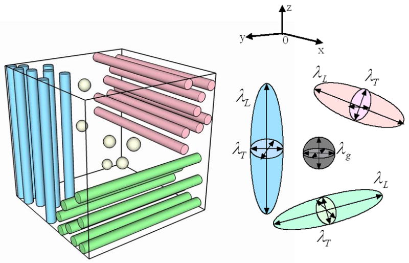
The multi-compartment model for the diffusion process. The three colored bundles (red, green, and blue) represent the axons in three orthogonal directions and the gray spherical balls represent the glial cells.

Assuming the exchange across compartments is relatively slow during the diffusion measurement time, the echo attenuations along the three local coordinates can be described as (3) [9], [18], [20]–[23].

$$\{\begin{array}{c}{f}_1\cdot {\mathit{e}}^{-b\cdot D_{\text{L}}}+f_2\cdot {\mathit{e}}^{-b\cdot D_{\text{T}}}+f_3\cdot {\mathit{e}}^{-b\cdot D_{\text{T}}}+(1-f_1-f_2-f_3)\cdot {\mathit{e}}^{-b\cdot D_{\gamma }}={\mathit{e}}^{-b\cdot D_1^{\text{eff}}}\\ f_1\cdot {\mathit{e}}^{-b\cdot D_{\text{T}}}+f_2\cdot {\mathit{e}}^{-b\cdot D_{\text{L}}}+f_3\cdot {\mathit{e}}^{-b\cdot D_{\text{T}}}+(1-f_1-f_2-f_3)\cdot {\mathit{e}}^{-b\cdot D_{\gamma }}={\mathit{e}}^{-b\cdot D_2^{\text{eff}}}\\ f_1\cdot {\mathit{e}}^{-b\cdot D_{\text{T}}}+f_2\cdot {\mathit{e}}^{-b\cdot D_{\text{T}}}+f_3\cdot {\mathit{e}}^{-b\cdot D_{\text{L}}}+(1-f_1-f_2-f_3)\cdot {\mathit{e}}^{-b\cdot D_{\gamma }}={\mathit{e}}^{-b\cdot D_3^{\text{eff}}}\\ f_i\in [0,1],(i=1,2,3);\sum _{i=1}^3{f}_i\le 1\end{array}$$ (3)

where f_i, (i=1,2,3) denote the volume fractions (VF) of the three axon compartments. For each WM voxel, the solutions of (3) (in terms of f₁, f₂ and f₃) indicate the local histological structure underlying the anisotropic transportation processes of both water molecules and electrical charges. D_y is the diffusion coefficient of the fourth isotropic compartment. For most WM voxels, D_y equals D_ℊ to account for the contribution from glial cells. However, for many voxels close to the WM boundary, the partial volume high-diffusivity CSF greatly affects the effective diffusion tensor and dominates the effects of glial cells. We classify a voxel with the partial volume CSF effect, if all the eigenvalues of the diffusion tensor are larger than the longitude diffusivity within an axon bundle (i.e. D_L). Accordingly, for all the CSF-contaminated voxels, we assume the fourth isotropic compartment has the same diffusion coefficient, D_C, as the CSF does.

In addition, all axon bundles are bathed in the interstitial fluid (ISF), which decreases the level of the diffusion anisotropy. In other words, a larger partial volume occupied by the ISF allows for the higher diffusivity perpendicular to the fiber direction (i.e. an increasing D_T). To account for the partial volume effect of the ISF while retaining the maximal local anisotropy, we vary D_T in (3) from D_T^min to D_T^max until ${\displaystyle \sum _{i=1}^3}{f}_i\le 1$ is satisfied.

For some voxels, ${\displaystyle \sum _{i=1}^3}{f}_i\le 1$ cannot be satisfied even if D_T=D_T^max, suggesting that the multi-compartment diffusion model fails to fit the measured diffusion tensor data. We classified these voxels as TYPE IV. It is also rarely possible that $D_i^{\text{eff}}<D_{\text{g}}(i=1,2,3)$, which is most likely due to the DT-MRI acquisition noise. We classified the corresponding voxels as TYPE VI. Table I summarizes the criteria and interpretation for each voxel type.

Table I.

The definitions of the six TYPEs and the histological structure each TYPE represents within the white matter (WM).

TYPE	DEFINITION				HISTOLOGICAL STRUCTURE REPRESENTED
	f1	f2	f3	Dieff (i=1,2,3)
I	≠0	=0	=0	[Dg, DL]	unidirectional bundles
II	≠0	≠0	=0	[Dg, DL]	two bundles crossing orthogonally
III	≠0	≠0	≠0	[Dg, DL]	three bundles crossing orthogonally
IV	f1 + f2 + f3 >1			[Dg, DL]	the reference bundles do not fit
V				[DL, ∞)	the WM contaminated by CSF partially
VI				(0, Dg]	experimental noise

Conductivity Model

Due to the similarity between the transportation processes of electrical charge carriers and water molecules, the conductivity tensors share the eigenvectors with the measured diffusion tensors [1]. Similar to (1), we can write the effective conductivity tensor as

$${\mathbf{\sigma }}^{\text{eff}}={\mathbf{S}}_{\sigma }\cdot \left[\begin{array}{ccc}{\sigma }_1^{\text{eff}}& 0& 0\\ 0& {\sigma }_2^{\text{eff}}& 0\\ 0& 0& {\sigma }_3^{\text{eff}}\end{array}\right]\cdot {\mathbf{S}}_{\sigma }^{\text{T}},$$ (4)

where S_σ= S_D.

The same multi-compartment model was used for the electrical conductivity. Since the transportation process of electrical charges primarily takes place in the extracellular space [4], the inter-compartment exchange is effectively much faster for the electrical conductivity than for the water diffusion. Therefore, we compute the eigenvalues of the effective conductivity as the weighted sums of the conductivity values associated with all compartments, as expressed in (5).

$$\{\begin{array}{c}{\sigma }_1^{\text{eff}}=f_1\cdot {\sigma }_{\text{L}}+f_2\cdot {\sigma }_{\text{T}}+f_3\cdot {\sigma }_{\text{T}}+f_4\cdot {\sigma }_{\gamma }\\ {\sigma }_2^{\text{eff}}=f_1\cdot {\sigma }_{\text{T}}+f_2\cdot {\sigma }_{\text{L}}+f_3\cdot {\sigma }_{\text{T}}+f_4\cdot {\sigma }_{\gamma }\\ {\sigma }_3^{\text{eff}}=f_1\cdot {\sigma }_{\text{T}}+f_2\cdot {\sigma }_{\text{T}}+f_3\cdot {\sigma }_{\text{L}}+f_4\cdot {\sigma }_{\gamma }\end{array}$$ (5)

The weighting coefficients are the volume fractions of all compartments determined in the diffusion model by solving (3). σ_L and σ_T are defined as the longitude and transverse conductivities in any axon compartment, respectively. σ_L is set to be a constant. σ_T is linearly related to D_T while it is confined to be between σ_T^min and σ_T^max, as expressed in (6),

$${\sigma }_{\text{T}}=D_T\cdot \frac{{\sigma }_{\text{T}}^{max}-{\sigma }_{\text{T}}^{min}}{D_{\text{T}}^{max}-D_{\text{T}}^{min}}+\frac{D_{\text{T}}^{max}\cdot {\sigma }_{\text{T}}^{min}-D_{\text{T}}^{min}\cdot {\sigma }_{\text{T}}^{max}}{D_{\text{T}}^{max}-D_{\text{T}}^{min}}$$ (6)

For TYPE I~IV, f₄=0. For TYPE V, σ_γ = σ_C where σ_C is the isotropic conductivity of the CSF compartment.

Data Acquisition

The MRI data for two subjects (twice for the second subject to verify the consistence of the algorithm) were obtained using a 3 Tesla Trio scanner (Siemens, Erlangen, Germany). A three-plane localizer sequence was acquired to position subsequent scans. Scans with T1 and proton density (PD) contrasts were collected for tissue registration. T1 images were acquired coronally, using a 3D MPRAGE sequence (TR=2530ms, TE=3.65ms, TI=1100ms, 224 slices, 1×1×1mm voxel, flip angle=7 degrees, FOV=256×176mm). PD weighted images were acquired axially using a hyper-echo turbo spin echo (TSE) sequence (TR=8550ms, TE=14ms, 80 slices, 1×1×2mm voxel, flip angle=120 degrees, FOV=256mm). DT-MRI data were acquired axially, aligned with the TSE images, using a dual spin echo, single shot, pulsed gradient, echo planar imaging sequence (TR=10500ms, TE=98ms, 64 contiguous slices, 2×2×2mm voxel, FOV=256mm, 2 averages, b value=1000s/mm²). Thirteen unique volumes were collected to compute the tensor: a b=0 s/mm² image and 12 images with diffusion gradients applied in 12 non-collinear directions: (Gx, Gy, Gz) = [1.0, 0.0, 0.5], [0.0, 0.5, 1.0], [0.5, 1.0, 0.0], [1.0, 0.5, 0.0], [0.0, 1.0, 0.5], [0.5, 0.0, 1.0], [1.0, 0.0, −0.5], [0.0, −0.5, 1.0], [−0.5, 1.0, 0.0], [1.0, −0.5, 0.0], [0.0, 1.0, −0.5], [−0.5, 0.0, 1.0]. A dual echo flash field map sequence with voxel parameters common to the DT-MRI was acquired and used to correct the DT-MRI data for geometric distortion caused by magnetic field inhomogeneity (TR=700ms, TE=4.62ms/7.08ms, flip angle=90 degrees, magnitude and phase difference contrasts).

Image Processing

The image data were processed using software (BET, FLIRT, FUGUE and FDT) from the FMRIB Software Library (http://www.fmrib.ox.ac.uk/). FDT was used to correct the diffusion-weighted images for misalignment and distortion caused by the effects of eddy currents. The geometric distortion caused by the magnetic field inhomogeneity was determined from the field map image, and FUGUE was then used to correct each of the 13 eddy current corrected diffusion images for this distortion. FDT was then used to compute the diffusion tensor from the 13 eddy current and distortion corrected diffusion images.

The brain was extracted from the T1 and PD acquisitions using BET, then aligned to the dewarped, b=0 s/mm² image using FLIRT, allowing for translations and rotations but no scaling or shear (6 Degrees of Freedom (DoF) fit).

Results

We evaluated the proposed volume fraction model by confirming the categorized voxels with existing knowledge of the WM histology. The WM voxels were categorized into six TYPEs (defined in Table I). The number and percentage of voxels in each TYPE are summarized as Table II. In Fig. 2, the voxels are also color coded as red, orange, yellow, blue, white and green, representing the TYPE I~VI, respectively. P1, P2a and P2b refer to the experimental data on the first subject and twice for the second subject respectively. For both subjects, TYPE II and III, altogether representing voxels with multidirectional fibers, account for over 85% of the WM voxels, in accordance with the fact that the intravoxel orientational heterogeneity is considerable under the typical voxel size of DT-MRI [15]–[17], [23]. The WM voxels with the partial CSF volume were found on the rim of the ventricles filled with the CSF. And the conductivity at the interior of the brain has a higher level of anisotropy than at the exterior, e.g., the splenium of corpus callousum (CCS) and internal capsule (IC) parts show less fiber crossing than other parts.

Table II.

The statistics of the WM voxels within each TYPE, including the number and the percentage (in the parentheses) of the voxels. P1, P2a and P2b refer to the experimental data on the first subject and twice for the second subject respectively.

Group	WM	TYPE I	TYPE II	TYPE III	TYPE IV	TYPE V	TYPE VI
P1	58866	257 (0.44%)	23755 (40.35%)	33346 (56.65%)	1581 (2.69%)	1434 (2.44%)	74 (0.13%)
P2a	79601	154 (0.19%)	20301 (25.50%)	49923 (62.72%)	3596 (4.52%)	9131 (11.47%)	92 (0.12%)
P2b	73501	121 (0.16%)	19751 (26.87%)	44833 (61.00%)	3473 (4.73%)	8706 (11.84%)	90 (0.12%)

Fig. 2.

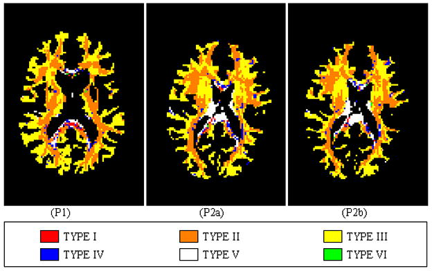
Distribution of the six types of voxels within WM for three groups of DT-MRI data. The slice is about 66mm below the vertex. P1, P2a and P2b refer to the experimental data on the first subject and twice for the second subject respectively.

Fig. 3 shows the distribution of each eigenvalue of the effective conductivity tensors σ^eff estimated by using all three algorithms (i.e. VC, Lin and VF). The VC algorithm resulted in the homogeneous distribution for each eigenvalue. This is obviously undesirable as it ignores the intravoxel orientational heterogeneity. Both the VF and Lin algorithms revealed similarly inhomogeneous distributions for all three eigenvalues. However, relative to the Lin’s results, we found in the VF’s results more voxels on the rim of the ventricles with a close-to-isotropic conductivity. This difference suggests the superiority of the VF algorithm over the Lin algorithm, in light of the fact that the partial volume effect of the CSF exists in those voxels around the ventricles and effectively accounts for a more isotropic conductivity. In addition, in the Lin’s results, the voxels at the rim of the ventricles also had very high values of σ₁^eff (over 2S/m), which is not reasonable since the CSF has the highest conductivity (1.79 S/m) among all the tissues in the brain. For all these voxels, the effective conductivity tensors extracted by using the VF algorithms all had eigenvalues no larger than the conductivity of CSF (1.79S/m) (see Fig. 4).

Fig. 3.

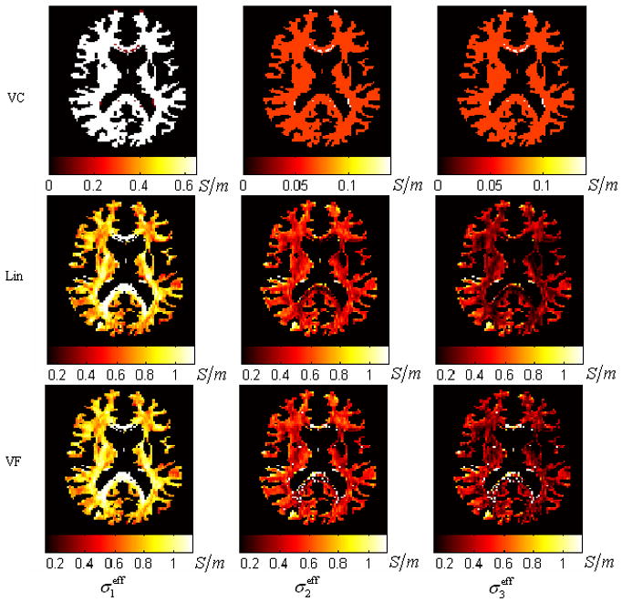
The distribution of the effective conductivity for the first group of experiment generated by the three algorithms: VC, Lin, and VF. This slice is about 66mm below the vertex. Three rows refer to the three algorithms. Three columns refer to the maps of the three sorted eigenvalues of the effective conductivity tensor.

Fig. 4.

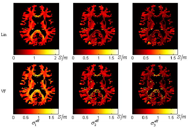
The distribution of the effective conductivity for the first group of experiment generated by the Lin and the VF. This slice is about 66mm below the vertex. Two rows refer to the two algorithms. And three columns refer to the maps of the three sorted eigenvalues of the effective conductivity tensor. The color bar scaled from 0 to the maximum eigenvalue of the conductivity tensor.

Discussion

Previous literatures suggested that the WM conductivity is 0.0585 S/m on average [25], and that its component perpendicular to the fiber direction is 0.125 S/m but nine times larger along the fiber direction [8]. These direct measurements also suggest that the conductivity of the cerebral WM varies among the locations within the WM and it also depends on each individual as well as the pathological or metabolizing condition of the brain. Therefore, mapping the WM conductivity from the noninvasive DT-MRI data is highly desirable.

Some existing algebraic relationships have been formulated based upon the micro-mechanism of relevant transport processes [2], [4], [5]. These algorithms often rely heavily on some microcosmic parameters which are difficult to obtain in practice, such as the in vivo intra-/extra-cellular conductivities. Some of these algorithms may also have to simplify the complicated relations as in a linear way. Although recently proposed volume constraints may help retain the histological structure to some degree [10], it often fails to consider the existence of fiber crossing and its variability across the WM volume.

In the present study, we proposed a new algorithm to extract the electrical conductivity tensor from the diffusion tensor measured through DT-MRI. By modeling the voxel-wise regional histological structure as a multi-compartment model, the proposed algorithm promises to be able to handle the intravoxel fiber crossing and the partial volume effects of the CSF. Our preliminary results based on the data acquired from two human subjects are in general agreement with our understanding about the WM histology and conductivity. The results also suggest that the proposed VF algorithm out-performs the existing Lin and VC algorithms, in face of the partial volume effect of the CSF and intravoxel orientation heterogeneity.

The diameter of an axon bundle is less than 10μm on average while the typical voxel size of DT-MRI is about 1 to 5 mm. According to the postmortem anatomic atlas [16] and some reported fiber tracking studies [11], [12], [17], [26], the axon fibers converge and diverge all along their specific tracts without any definite boundary. For example, the inferior longitudinal and fronto-occipital fasciculi share most of their projections at the occipital lobe and begin to diverge at the posterior temporal lobe as the former stretches to the temporal lobe while the latter stretches to the frontal lobe. Also, the widely scattering cortical U fibers, which are hard to tract for its irregular passages, greatly increase the possibility of the fiber-crossing. Therefore, out finding that about 85% of voxels have various crossing fiber structures appears to be reasonable, although it is certainly desirable to further validate or confirm this finding.

As shown in Fig. 3, the proposed VF algorithm provides more reasonable WM conductivity estimates than the VC algorithm, since the latter ignores the intravoxel orientational discrepancies among different voxels by assuming a homogeneous distribution for each eigenvalue of the conductivity tensor. The conductivity distributions estimated by the VF algorithm and the Lin algorithm appear to be mostly similar. However, the Lin algorithm produces more errors for the voxels on the border of the WM and the CSF, as seen in Fig. 4.

In summary, we have proposed a new algorithm for estimating anisotropic electrical conductivity based on the DT-MRI data. The pilot experimental study in two healthy human subjects suggests that the proposed VF algorithm provides a good estimate of the WM anisotropic conductivity, and merits further investigation.

References

- 1.Basser PJ, Mattiello J, LeBihan D. MR diffusion tensor spectroscopy and imaging. Biophys J. 1994 Jan;66:259–267. doi: 10.1016/S0006-3495(94)80775-1. [DOI] [PMC free article] [PubMed] [Google Scholar]
- 2.Tuch DS, Wedeen VJ, Dale AM, George JS, Belliveau JW. Conductivity mapping of the human brain using diffusion tensor MRI. Proc Natl Acad Sci USA. 2001 Sep;98:11697–11701. doi: 10.1073/pnas.171473898. [DOI] [PMC free article] [PubMed] [Google Scholar]
- 3.Sen AK, Torquato S. Effective conductivity of anisotropic two- phase composite media. Phys Rev, B Condens Matter. 1989 Mar;39:4504–4515. doi: 10.1103/physrevb.39.4504. [DOI] [PubMed] [Google Scholar]
- 4.Tuch DS, Wedeen VJ, Dale AM, George JS, Belliveau JW. Conductivity mapping of biological tissue using diffusion MRI. Ann N Y Acad Sci. 1999 Oct;888:314–316. doi: 10.1111/j.1749-6632.1999.tb07965.x. [DOI] [PubMed] [Google Scholar]
- 5.Sekino M, Yamaguchi K, Iriguchi N, Ueno S. Conductivity tensor imaging of the brain using diffusion-weighted magnetic resonance imaging. J Appl Phys. 2003 May;93:6730–6732. [Google Scholar]
- 6.Sekino M, Inoue Y, Ueno S. Magnetic resonance imaging of mean values and anisotropy of electrical conductivity in the human brain. Neurol Clin Neurophysiol. 2004 Nov;55:1–5. [PubMed] [Google Scholar]
- 7.Wolters CH. PhD thesis. Leipzig Univ; Leipzig: 2003. Influence of tissue conductivity inhomogeneity and anisotropy to EEG/MEG based source localization in the human brain. [Google Scholar]
- 8.Nicholson PW. Specific impedance of cerebral white matter. Exp Neurol. 1965 Dec;13:386–401. doi: 10.1016/0014-4886(65)90126-3. [DOI] [PubMed] [Google Scholar]
- 9.Alexander AL, Hasan KM, Lazar M, Tsuruda JS, Parker DL. Analysis of Partial Volume Effects in Diffusion-Tensor MRI. Magn Reson Med. 2001 May;45:770–780. doi: 10.1002/mrm.1105. [DOI] [PubMed] [Google Scholar]
- 10.Wolters CH, Anwander A, Tricoche X, Weistein D, Koch MA, MacLeod RS. Influence of tissue conductivity anisotropy on EEG/MEG field and return current computation in a realistic head model: a simulation and visualization study using high-resolution finite element modeling. Neuroimage. 2006 Apr;30:813–826. doi: 10.1016/j.neuroimage.2005.10.014. [DOI] [PubMed] [Google Scholar]
- 11.Meyer JW, Makris N, Bates JF, Caviness VS, Kennedy DN. MRI-based topographic parcellation of human cerebral white matter: I technical foundations. Neuroimage. 1999 Jan;9:1–17. doi: 10.1006/nimg.1998.0383. [DOI] [PubMed] [Google Scholar]
- 12.Makris N, Meyer JW, Bates JF, Yeterian EH, Kennedy DN, Caviness VS. MRI-based topographic parcellation of human cerebral white matter and nuclei: II. Rationale and applications with systematics of cerebral connectivity. Neuroimage. 1999 Jan;9:18–45. doi: 10.1006/nimg.1998.0384. [DOI] [PubMed] [Google Scholar]
- 13.Basser PJ, Mattiello J, LeBinhan D. Estimation of the effective self-diffusion tensor from the NMR spin echo. J Magn Reson B. 1994 Mar;103:247–254. doi: 10.1006/jmrb.1994.1037. [DOI] [PubMed] [Google Scholar]
- 14.Le Bihan D, Mangin JF, Poupon C, Clark CA, Pappata S, Molko N, Chabriat H. Diffusion tensor imaging: concepts and applications. J Magn Reson Imaging. 2001 April;13:534–546. doi: 10.1002/jmri.1076. [DOI] [PubMed] [Google Scholar]
- 15.Bear MF, Connors BW, Paradiso MA. Neuroscience: Exploring the Brain. 2. Hagerstown, MD: Lippincott Williams & Wilkins; 2001. [Google Scholar]
- 16.Nieuwenhuys R, Voogd J, van Huijzen C. The human central nervous system. Berlin, Germany: Springer-Verlag; 1983. [Google Scholar]
- 17.Wakana S, Jiang H, Nagae-Poetscher L, van Zijl PC, Mori S. Fiber tract-based atlas of human white matter anatomy. Radiology. 2004 Jan;230:77–87. doi: 10.1148/radiol.2301021640. [DOI] [PubMed] [Google Scholar]
- 18.Stanisz GJ, Szafer A, Wright GA, Henkelman RM. An analytical model of restricted diffusion in bovine optic nerve. Magn Reson Med. 1997 Jan;37:103–111. doi: 10.1002/mrm.1910370115. [DOI] [PubMed] [Google Scholar]
- 19.Shimony JS, McKinstry RC, Akbudak E, Aronovitz JA, Snyder AZ, Lori NF, Cull TS, Conturo TE. Quantitative diffusion-tensor anisotropy brain MR imaging: normative human data and anatomic analysis. Radiology. 1999 Sep;212:770–784. doi: 10.1148/radiology.212.3.r99au51770. [DOI] [PubMed] [Google Scholar]
- 20.Nicholson C. Diffusion and related transport mechanisms in brain tissue. Rep Progr Phys. 2001;64:815–884. [Google Scholar]
- 21.Beaulieu C. The basis of anisotropic water diffusion in the nervous system – a technical review. NMR Biomed. 2002 Nov;15:435–455. doi: 10.1002/nbm.782. [DOI] [PubMed] [Google Scholar]
- 22.Clark CA, Le Bihan D. Water diffusion compartmentation and anisotropy at high b values in the human brain. Magn Reson Med. 2000 Dec;44:852–859. doi: 10.1002/1522-2594(200012)44:6<852::aid-mrm5>3.0.co;2-a. [DOI] [PubMed] [Google Scholar]
- 23.Tuch DS, Reese TG, Wiegell MR, Makris N, Belliveau JW, Wedeen VJ. High angular resolution diffusion imaging reveals intravoxel white matter fiber heterogeneity. Magn Reson Med. 2002 Oct;48:577–582. doi: 10.1002/mrm.10268. [DOI] [PubMed] [Google Scholar]
- 24.Haueisen J, Tuch DS, Ramon C, Schimpf PH, Wedeen VJ, Seorge JS, Belliveau JW. The influence of brain tissue anisotropy on human EEG and MEG. Neuroimage. 2002 Jan;15:159–166. doi: 10.1006/nimg.2001.0962. [DOI] [PubMed] [Google Scholar]
- 25.Gabriel C, Gabriel S, Corthout E. The dielectric properties of biological tissues: I. Literature survey. Phys Med Biol. 1996 Nov;41:2231–2249. doi: 10.1088/0031-9155/41/11/001. [DOI] [PubMed] [Google Scholar]
- 26.Mori S, Crain BJ, Chacko VP, van Zijl PC. Three-Dimensional Tracking of Axonal Projections in the Brain by Magnetic Resonance Imaging. Ann Neurol. 1999 Feb;45:265–269. doi: 10.1002/1531-8249(199902)45:2<265::aid-ana21>3.0.co;2-3. [DOI] [PubMed] [Google Scholar]
- 27.Pierpaoli C, Jezzard P, Basser PJ, Barnett A, Di Chiro G. Diffusion tensor MR imaging of the human brain. Radiology. 1996 Dec;201:637–648. doi: 10.1148/radiology.201.3.8939209. [DOI] [PubMed] [Google Scholar]
- 28.Frank LR. Characterization of anisotropy in high angular resolution diffusion-weighted MRI. Magn Reson Med. 2002 Jun;47:1083–1099. doi: 10.1002/mrm.10156. [DOI] [PubMed] [Google Scholar]