Modeling Adolescent Drug-Use Patterns in Cluster-Unit Trials With Multiple Sources of Correlation Using Robust Latent Class Regressions

Abstract

PURPOSE

The purpose of the study is to examine variation in adolescent drug-use patterns by using latent class regression analysis and evaluate the properties of an estimating-equations approach under different cluster-unit trial designs.

METHODS

A set of second-order estimating equations for latent class models under the cluster-unit trial design are proposed. This approach models the correlation within subclusters (drug-use behaviors), but ignores the correlation within clusters (communities). A robust covariance estimator is proposed that accounts for within-cluster correlation. Performance of this approach is addressed through a Monte Carlo simulation study, and practical implications are illustrated by using data from the National Evaluation of the Enforcing Underage Drinking Laws Randomized Community Trial.

RESULTS

The example shows that the proposed method provides useful information about the heterogeneous nature of drug use by identifying two subtypes of adolescent problem drinkers. A Monte Carlo simulation study supports the proposed estimation method by suggesting that the latent class model parameters were unbiased for 30 or more clusters. Consistent with other studies of generalized estimating equation (GEE) estimators, the robust covariance estimator tended to underestimate the true variance of regression parameters, but the degree of inflation in the test size was relatively small for 70 clusters and only slightly inflated for 30 clusters.

CONCLUSIONS

The proposed model for studying adolescent drug use provides an alternative to standard diagnostic criteria, focusing on the nature of the drug-use profile, rather than relying on univariate symptom counts. The second-order GEE-type estimation procedure provided a computationally feasible approach that performed well for a moderate number of clusters and was consistent with prior studies of GEE under the generalized linear model framework.

INTRODUCTION

Large-scale epidemiologic surveys of adolescent drug use typically involve asking a series of self-report questions about amount, frequency, and problems associated with drug use. Goals of these studies are to characterize adolescent drug users and identify factors that influence adolescent drug use to obtain a better understanding of the epidemiologic characteristics of adolescent drug use in community populations. A common approach for characterizing drug users is the use of standard diagnostic criteria, most notably the Diagnostic and Statistical Manual of Mental Disorders (DSM) (1), to identify drug-dependent individuals. These criteria are based on the consensus of researchers about which patterns of behaviors or physiologic characteristics constitute symptoms of drug dependence. A diagnosis of drug dependence is made when an individual endorses three or more clinical features of the drug-dependence syndrome. Not only is there little empirical justification for this definition of drug dependence, but by giving all criteria equal weight, clinically important subgroups of drug users may be ignored. For example, two individuals meeting criteria for drug dependence may show different patterns of behavior. Using data from the National Household Survey of Drug Abuse, Reboussin and Anthony (2) found evidence for two different subtypes of cocaine dependence in recent onset cocaine users, each showing qualitatively different clinical profiles.

Although standard diagnostic criteria are useful in research for making comparisons between studies and in clinical practice for making decisions about treatment, there is good reason in studies of adolescent drug use to consider an alternative to DSM-type criteria. Clinical experts on DSM task panels tend to base their choice of criteria on experiences with adults seeking treatment for drug dependence. Typically, these criteria have not been validated in community samples of adolescents. Researchers reported evidence that DSM-like clinical features of cocaine and heroin dependence observed in community samples might be considerably different from corresponding patterns observed in samples of patients seeking drug dependence treatment (3). Still others showed that many youth who experience harmful consequences as a result of drinking do not meet clinical dependence criteria (4-7).

There also is evidence to suggest that adolescents endorse clinical features of tobacco and alcohol dependence at different rates than adults. Martin et al. (8) found that adolescent drinkers reported fewer withdrawal symptoms and medical problems, whereas Chung et al. (5) found evidence for more reporting of drinking in hazardous situations. Prokhorov et al. (9) reported adolescent nicotine dependence rates half those of adults, although the majority of adolescents reported being addicted to smoking. These researchers also found evidence for less intense and pervasive smoking patterns among adolescents.

Evidence of differences in drug-use patterns between adolescents and adults and between community-based and treatment-seeking populations, as well as the possibility that diagnostic criteria may fail to identify potentially meaningful subgroups of adolescent drug users, emphasizes the importance of empirically examining drug-use patterns in community samples of adolescents. In this report, we present an empirically based method for explaining the heterogeneity in patterns of drug use in terms of underlying latent classes. Latent class analysis (LCA) is a statistical approach used to create homogeneous groups of adolescents with similar drug-use patterns and determine the influence of various factors on risk for showing these drug-use patterns.

Our focus is on cluster-unit trials aimed at preventing adolescent drug use. Cluster-unit trials are implemented when the focus of an intervention is its impact on socially or geographically defined groups. For example, schools are natural settings for many efforts to reduce adolescent drug use, with virtually all adolescents attending school. Reducing adolescent drug use also is consistent with educational objectives, thereby allowing interventions to be incorporated easily into school curricula (10). Another pathway to reduce adolescent drug use is through public policy. Intervention programs may focus on evaluating the impact of public policy on preventing adolescent drug use at the state or county level (11). In both these designs, random assignment of individuals to intervention or control conditions is nearly impossible. In the case of school-based programs, it would be logistically difficult for school administrators to provide an intervention to a subset of students from different classrooms. Social mixing of students outside the classroom also is likely to contaminate the control condition with intervention messages. For interventions targeted at public policy, it similarly would be difficult to limit effects of public policy to only adolescents in a state or county who had been assigned to the intervention condition. As a result, the standard approach in these types of studies is to assign the intervention at the school or community level. This distinguishes it from subject-level clinical trials in which assignment is at the individual level.

There are two potential sources of correlation in cluster-unit trials of drug-use patterns (Fig. 1); correlation of drug-use behaviors within individuals (subcluster) ρ₁ and correlation between individuals from the same school or community (cluster) ρ₂. ρ₁ is the scientific focus of our investigation, but failure to account for ρ₂ in regression analyses could result in inflated type I error rates (12). The generalized estimating equation (GEE) is a popular approach to account for cluster-correlated data in the generalized linear model setting (13). Most often it is applied to longitudinal data, for which correlation among repeated measures is a nuisance and the focus is regression parameters. GEE estimators have the desirable property of asymptotic robustness of the covariance matrix of regression coefficients to misspecification of the covariance matrix of correlated data. This robustness property allows for specification of simple “working” covariance matrices among clustered responses, such as independence and exchangeable (i.e., constant correlation). Qaqish and Liang (14) developed a set of quadratic or second-order generalized estimating equations (GEE2) for correlated responses with multiple levels of nesting by using the generalized linear model framework. This approach is recommended when modeling the dependence structure is of interest. In a similar manner, Reboussin and Anthony (15) developed a set of GEE2-type estimating equations for the latent class regression model in which repeated measures were nested within subclusters (e.g., behaviors) that were nested within clusters (individuals). Modeling of pairwise associations between behaviors forms the basis for these models, whereas correlation between individuals is considered a nuisance.

FIGURE 1.

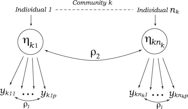
Sources of correlation in cluster-unit trials of drug-use patterns.

As mentioned, robustness properties of GEEs are asymptotic and originally were motivated by longitudinal studies with large numbers of clusters (individuals) of small size (repeated observations). The cluster-unit trial framework is different, with the study design often involving a small number of clusters (e.g., schools or communities) of large size (individuals). Numerous simulation studies indicated that GEE tends to underestimate to varying degrees the variance of regression parameters when the number of clusters is less than 40, with resulting hypothesis tests and confidence intervals too liberal (10, 16-18). This bias occurs because the robust covariance estimator uses residuals (observed minus expected) at the cluster level to calculate the true covariance matrix of correlated responses. In addition, the GEE2 approach was shown to be computationally infeasible as the cluster size gets large (19). In this report, we present a modified version of the GEE2-type estimating equations of Reboussin and Anthony (15) for latent class models under the cluster-trial design. In this framework, behaviors (e.g., drug use) are nested within subclusters (individuals) that are nested within clusters (communities). This approach models the correlation within subcluster, but ignores the correlation within cluster at the estimation stage, thereby avoiding the computational complexity of GEE2-type approaches associated with large cluster sizes. A robust covariance estimator is proposed that accounts for within-cluster correlation. We address the performance of this proposed approach through Monte Carlo simulation study under various cluster-trial designs. Practical implications of results are illustrated by using data from the National Evaluation of the Enforcing Underage Drinking Laws Randomized Community Trial (EUDL-CT).

REGRESSION MODELS

Models for Within-Subcluster Correlation

Let y_kij be a binary response for the jth observation j = 1,...,p within the ith subcluster i = 1,...,n_k of the kth cluster k = 1,...,K. For our purposes, y_kij = 1 if drug behavior j is reported by youth i within community k and O if not. We refer to y_ki = (y_ki1,...,y_kip)’ as the drug-behavior profile at the sub-cluster level. Our primary scientific interest is to identify subgroups of youth with similar drug-behavior profiles by using LCA. LCA is a statistical approach for explaining the structure in multivariate response profiles in terms of latent (or unobserved) classes. This is in contrast to latent trait models in which heterogeneity in response profiles is described in terms of an underlying continuous trait. This type of dimensional approach cannot be used to divide individuals into homogenous subgroups. In the LCA framework, associations among drug behaviors within an individual (subcluster) are assumed to be the result of an underlying subclassification of youth into different drug-behavior sub-types (classes). In a statistical sense, this means that drug behaviors are mutually independent after latent class membership is conditioned out or that relationships between drug behaviors are due to their relationship to the latent class variable. In the context of adolescent drinking, you can see how we might characterize latent classes as problem-drinking subtypes if they explain the observed relationships between alcohol consumption, alcohol risk behaviors, and problems from drinking. This axiom is the hallmark of LCA and is termed local independence. The desired result from making such an assumption is a set of homogenous classes of youth, each with its own set of drug-behavior response probabilities. LCA defines homogeneity in terms of probabilities such that individuals are similar to each other because their drug-behavior profiles are generated from the same probability distribution (20, 21). Because latent class membership is not observed without error, this axiom is not verifiable; however, its adequacy compared under various class assumptions is discussed in “Data Example.” For estimation purposes, the number of classes is assumed to be known.

There are two sets of parameters to be estimated in LCA modeling: π_m = P(η_ki = m) is the prevalence of drug-behavior class m and π_jm = P(y_kij = 1 | η_ki = m) is the response probability that a randomly selected youth from class m reports drug behavior j. Response probabilities π_jm aid in the interpretation of latent classes by characterizing drug behaviors of individuals within a particular latent class.

Covariance between drug-use behaviors j and h under the local independence assumption is a function of these LCA parameters and is given by:

$${\sigma }_{kijh}=\sum _{m=1}^{\mathrm{C}}{p}_{jm}{p}_{hm}{\pi }_m-\sum _{m=1}^{\mathrm{C}}{p}_{jm}{\pi }_m\sum _{m=1}^{C0}{p}_{hm}{\pi }_m$$

where C is number of latent classes and ${\mu }_{kij}=E\left[Y_{kij}\right]={\sum }_{m=1}^{\mathrm{C}}{p}_{jm}{\pi }_m$.

In addition to observing a set of responses to a series of questions regarding drug behaviors, we also might observe a set of q risk factors thought to be possible determining factors of class membership. Scientific interest then focuses on how the latent class prevalences π_m depend on suspected risk factors. A baseline-category logistic regression model for marginal latent class prevalences is given by:

$$\log \frac{{\pi }_m\left(x_{ki}\right)}{{\pi }_1\left(x_{ki}\right)}={\alpha }_m+x_{ki}^{\prime }{\gamma }_m$$ (1)

where π_m(χ_ki) = P(η_ki = m|χ_ki), m = 2 ..., C and χ_ki1 = (χ_ki1,...χ_kiq) is a q × 1 covariate vector that can include cluster-level and subcluster-level covariates.

Ignoring for a moment the within-cluster correlation, we propose solving the following second-order estimating equations U(θ) for the parameters of interest θ = (α, γ, p) that incorporate information from both the first and second moments of the observed drug-behavior profile at subcluster-level y_ki:

$$\begin{array}{cc}\hfill U\left(\theta \right)=& \sum _{k=1}^K\sum _{i=1}^{n_k}{U}_{ki}=\sum _{k=1}^K\sum _{i=1}^{n_k}\left(\frac{\partial {\mu }_{ki}\left(\theta \right)}{\partial \theta },\frac{\partial {\sigma }_{ki}\left(\theta \right)}{\partial \theta }\right)R_{ki}{\left(\theta \right)}^{-1}\hfill \\ \hfill & \left(\begin{array}{c}{y}_{ki}-{\mu }_{ki}\left(\theta \right)\hfill \\ w_{ki}\left(\theta \right)-{\sigma }_{ki}\left(\theta \right)\hfill \end{array}\right)=0\hfill \end{array}$$ (2)

where w_ki={(y_kij – μ_kij)(y_kih – μ_kih); j < h = 1,..., p} and R_ki is a p(p + 1)/2 by p(p + 1)/2 within-subcluster working covariance matrix of y_ki and w_ki. This is unlike GEEs for generalized linear models that only use information in the first moments. Information in the second moments is necessary for identification of latent class model parameters in which covariance between drug-use behaviors within an individual is of scientific interest. Following the work of Qaqish and Liang (14) and Reboussin and Anthony (15), second-order estimating equations in (2) yield consistent and asymptotically normal parameter estimates as long as the first two moments are specified correctly, even if within-subcluster working covariance matrix assumptions are violated. Various simplifying assumptions can be made to ease computations. In particular, we assume working independence within a subcluster for R_ki in both our data example and simulation study to follow.

Models for Within-Cluster Correlation

Although correlation of drug behaviors within a community is an interesting area of research, it is not the scientific focus of our study (22, 23). However, failure to account for this correlation among youths within a community could result in inflated type I error rates (12). If we assume working independence between individuals within a community k, we can use estimating equations in (2) that ignore cluster-level correlation and still obtain consistent parameter estimates. Although estimating equations in (2) only incorporate information in the cross-products of responses within a subcluster, w_ki, and may result in a loss of efficiency, we expect most of the information regarding latent class prevalences and the appropriateness of the local independence assumption to be contained in associations between responses within a subcluster.

The asymptotic covariance of the parameter estimates $\widehat{\theta }$ accounts for the correlation within clusters by incorporating the corrected cross-products for different participants within clusters in the middle term of the variance. A similar sandwich covariance estimator for cluster-trial designs in the generalized linear model framework is given by Miller et al. (24). The asymptotically robust covariance estimator for $\widehat{\theta }$ estimated by solution of (2) is given by:

$$\begin{array}{cc}\hfill & {\left(\sum _{k=1}^N\sum _{i=1}^{n_k}{D}_{ki}^{\prime }{R}_{ki}^{-1}{D}_{ki}\right)}^{-1}(\sum _{k=1}^K\left(\sum _{i=1}^{n_k}{U}_{ki}\left(\widehat{\theta }\right)\right)\phantom{)}\hfill \\ \hfill & \times \phantom{(}{\left(\sum _{i=1}^{n_k}{U}_{ki}\left(\widehat{\theta }\right)\right)}^{\prime }){\left(\sum _{k=1}^K\sum _{i=1}^{n_k}{D}_{ki}^{\prime }{R}_{ki}^{-1}{D}_{ki}\right)}^{-1}\hfill \end{array}$$

where D_ki is the matrix of first-order derivatives of the first two moments with respect to θ and θ is replaced by its estimate $\widehat{\theta }$.

DATA EXAMPLE

LCA is applied to data collected at baseline from the EUDL-CT. This trial, funded by the US Office of Juvenile Justice and Delinquency Prevention, is designed to determine effects of a local coalition-based approach to implementing “best” or “most promising” strategies for increasing enforcement of laws related to underage drinking (25). Five states were funded to participate in the EUDL-CT. Nominated communities in each funded state were matched based on population; median family income; percentages of the population that are black, Hispanic, speak Spanish, and currently in college; and (for states for which it was available) the arrest rate of 16- to 20-year-olds for liquor law violations. After creation of 35 matched pairs, communities within a pair were randomly assigned to either the intervention or comparison condition. A total of 7103 youths aged 14 to 20 years from 70 communities were surveyed by telephone at baseline between January 2004 and July 2004. Median number of youth surveyed per community was 105, with a range of 65 to 137.

We characterized underage drinking patterns by considering binary responses to seven questions about the extent of alcohol consumption, alcohol risk behaviors, and physical and social problems from drinking. This approach is consistent with a similar analysis performed on a sample participating in a nonrandomized version of the EUDL-CT (26). “Regular drinking” was assessed by asking “On how many occasions have you had alcohol to drink in the last 30 days?” Respondents were characterized as regular drinkers if they reported drinking on six or more occasions in the past 30 days. “Binge drinking” was assessed by asking the respondent “Think back over the past 2 weeks. How many times have you had five or more drinks in a row? A drink is a glass of wine, a bottle of beer, a shot glass of liquor, a mixed drink, or a wine cooler.” Respondents who reported binge drinking one or more times in the past 2 weeks were contrasted with respondents who did not report binge drinking in the past 2 weeks. “Drunkenness” was assessed by asking “Over the past 12 months, on how many days have you gotten drunk or ‘very very high’ on alcohol? Would you say every day or almost every day, 3 to 5 days a week, 1 or 2 days a week, 2 or 3 days a month, once a month or less, 1 or 2 days in the past 12 months, or never.” Respondents who reported getting drunk at least 2 or 3 days a month were contrasted with all others. “Driving after drinking” was assessed by asking “During the past 30 days, how many times (if any) have you driven after drinking two or more drinks in an hour or less?” Respondents who reported driving at least once after drinking in the past 30 days were compared with all others. Respondents then were asked if they had any of the following experiences after they were drinking. For each problem, adolescents who reported experiencing a problem during the past 12 months were contrasted with all others. “Physical problems” included asking “Have you passed out?,” “Were you unable to remember what happened while drinking?,” and “Have you had a headache or hangover?” “Social problems” included “Were you cited or arrested for drinking, possessing, or trying to buy alcohol?,” “Have you missed any school due to drinking?,” “Were you warned by a friend about your drinking?,” “Did you break or damage something?,” and “Were you punished by your parents or guardian?” Based on exploratory analyses, the five social problems from drinking were combined into a single indicator of any social problems from drinking because of their low prevalence and lack of discriminatory power. There also was a strong local dependency between reporting passing out from drinking and being unable to remember what happened. This likely occurs because both questions are measuring closely related traits; therefore, we similarly replaced these two items by a single item that was positive if the response to either question was positive.

This analysis is based on a sample of 1678 past-30-day underage drinkers from 70 communities, with number of drinkers per community ranging from 12 to 41 and a median of 22.5. A series of latent class models were fit to the data. We started with the most parsimonious one-class model (“all drinkers the same”) and fit successive models with an increasing number of latent classes to determine the most parsimonious model that provided adequate fit to the data. Goodness of fit of various models was evaluated with an emphasis on Akaike information criteria (AIC), a global fit index that combines goodness of fit and parsimony. Based on a recommendation of Lin and Dayton (27), AIC is believed to be more appropriate than Bayesian information criteria when there are complex models of the type encountered in this research. AIC require a likelihood for model comparison and GEE is non-likelihood based. Pan (28) proposed a version of the AIC for GEEs that is based on the quasi-likelihood under the working independence model with $\widehat{\theta }$ estimated by using any general working correlation structure in GEE. We consider a modified version of Pan's AIC for the GEE2-type estimating equations in (2)

$$\begin{array}{cc}\hfill AIC=& \sum _{k=1}^K\sum _{i=1}^{n_k}(y_{ki}-{\mu }_{ki}\left(\widehat{\theta }\right))V^{-1}(y_{ki}-{\mu }_{ki}\left(\widehat{\theta }\right))\hfill \\ \hfill & +\sum _{k=1}^K\sum _{i=1}^{n_k}(w_{ki}\left(\widehat{\theta }\right)-{\sigma }_{ki}\left(\widehat{\theta }\right))W^{-1}(w_{ki}-{\sigma }_{ki}\left(\widehat{\theta }\right))+2r\hfill \end{array}$$ (3)

where V and W are the working covariance matrices of y_ki and w_ki calculated under independence and r is total number of parameters. We performed a simple simulation study to evaluate performance of the AIC given in equation 3. Briefly, we generated 1000 data sets for a two-class model and successively fit one-, two-, and three-class models. Generation of data for latent class models is discussed in greater detail in “Simulation Study.” For each of 1000 data sets, the AIC in equation 3 correctly chose the two-class model as providing the best fit to the data.

Based on AIC criteria in equation 3 for which smaller indicates better fit, the three-class model fit was found to be superior to the two-class model fit for the EUDL-CT data example. The four-class model solutions were highly dependent on starting values, suggesting the model is not identifiable with our sample size or that the four-class model is an overparameterization. Parameter estimates and AIC values for the two- and three-class models are listed in Table 1. The two-class model suggests that about 40% of underage drinkers are engaging in problem drinking, i.e., drinking behavior associated with physical and social problems. The three-class model provides evidence for two subtypes of underage problem drinkers: risky drinkers (prevalence, 33%) and regular drinkers (prevalence, 31%). Of risky problem drinkers, an estimated 30% binged in the past 2 weeks and 41% had gotten drunken 2 to 3 days per month during the past year. Regular problem drinkers are characterized by underage drinkers who are significantly more likely to show risky drinking behaviors, and approximately half drank at least 6 days in the past month. These results are consistent with those of Reboussin et al. (26) in a sample of 16- to 20-year-olds participating in a nonrandomized version of this study.

TABLE 1.

Estimated response probabilities (p) and class prevalences (π) for two-and-three class models of underage drinking

	Two-class model		Three-class model
	Class 1	Class 2	Class 1	Class 2	Class 3
Regular drinking	0.01	0.42	0.01	0.03	0.51
Binge drinking	0.15	0.85	0.10	0.30	0.93
Drunkenness	0.19	0.91	0.13	0.41	0.97
Drove after drinking	0.02	0.26	0.03	0.04	0.31
Passed out/forgot	0.26	0.85	0.02	0.72	0.80
Headache/hangover	0.51	0.88	0.33	0.86	0.82
Social problems	0.22	0.58	0.15	0.41	0.57
Class prevalence	0.60	0.40	0.36	0.33	0.31
AIC	47,265.5		47,208.9

AIC = Akaike information criteria.

For both the two- and three-class models, the probability of being a member of an underage drinking class was modeled as a function of subcluster- and cluster-level covariates according to equation 1. χ_ki1 and χ_ki2 are subcluster-level covariates where χ_ki1 = 1 for males and 0 for females and χ_ki2 is an individual's age at baseline centered about its mean. χ_ki3 is a cluster-level covariate and is equal to 1 for communities designated as urban and 0 otherwise. Latent class model parameters were estimated by using the GEE2-type approach in equation 2.

Listed in Table 2 are the latent class logistic regression parameter estimates using the GEE2-type approach for the two-class model. Standard error estimates and p-values for Wald-type tests also are listed in Table 2 for the naive variance estimator that ignores correlation both within sub-clusters and within clusters, the robust variance estimator that accounts for the within-subcluster correlation ρ₁ (in this case, the correlation of drug behaviors within individuals), and the robust variance estimator that adjusts for correlation of behaviors within subjects and the correlation within-cluster ρ₂. Being male and older age were both significantly associated with increased risk for being a problem drinker, with odds ratios of 1.54 (e^0.435) and 1.49 (e^0.397), respectively. Living in an urban community was associated with decreased risk for being a problem drinker compared with living in a nonurban community, but this association was not statistically significant.

TABLE 2.

Latent class logistic regression results for a two-class model of underage drinking using a GEE2-type approach with naive, within-subcluster–and within-cluster–adjusted covariance estimators

		Naive independence		Robust within-subcluster		Robust within-cluster
	Estimate	SE	p	SE	p	SE	p
Male	0.435	0.062	< 0.001	0.122	< 0.001	0.125	0.001
Age	0.397	0.032	< 0.001	0.062	< 0.001	0.062	< 0.001
Urban	−0.104	0.066	0.115	0.129	0.420	0.148	0.482

GEE2 = second-generation generalized estimating equation; SE = standard error.

Results for the three-class model are listed in Table 3 and are similar. Being male and older age were associated with increased risk for being both a risky problem drinker (odds ratios, 1.3 and 1.1, respectively) and a regular problem drinker (odds ratios, 2.5 and 2.1, respectively). However, increased risk for being a risky problem drinker with older age was not statistically significant (p = 0.180). Similar to the two-class model, living in an urban community was associated with decreased risk for being a problem drinker (both risky and regular), but this association was not statistically significant.

TABLE 3.

Latent class logistic regression results for a three-class model of underage drinking using a GEE2-type approach with the naive, within-subcluster, and within-cluster—adjusted covariance estimators

		Naive independence		Robust within—subcluster		Robust within-cluster
	Estimate	SE	p	SE	p	SE	p
Class 2 versus 1
Male	0.260	0.079	0.001	0.126	0.039	0.110	0.018
Age	0.090	0.042	0.042	0.067	0.205	0.064	0.180
Urban	−0.156	0.081	0.056	0.137	0.256	0.152	0.305
Class 3 versus 1
Male	0.913	0.113	<0.001	0.219	<0.001	0.237	<0.001
Age	0.752	0.072	<0.001	0.116	<0.001	0.106	<0.001
Urban	−0.229	0.108	0.033	0.208	0.270	0.254	0.366

GEE2 = second-order generalized estimating equation.

The within-subcluster robust covariance estimator gave larger standard errors than the naive estimator that ignores all sources of correlation, as would be predicted. For the three-class model, the effect of age on risky problem drinking and the effect of living in an urban community on both risky and regular problem drinking were no longer significant after adjustment for within-subcluster correlation. Use of the within-cluster adjusted covariance estimator had only a small effect on standard errors and estimated p. This is not surprising given the small degree of correlation estimated within clusters (range, 0.0028 to 0.0221). However, the greatest effect was for the cluster-level covariate, as would be predicted from simulation results presented in the next section. Interestingly, for the three-class model, ignoring cluster-level correlation resulted in larger standard errors in some instances for subcluster-level covariates.

SIMULATION STUDY

Data Generation

To examine the GEE2-type approach for latent class models under various cluster-unit trial designs, we performed a Monte Carlo simulation study for a two-class model. A logistic regression model similar to the example was used to model latent class prevalences:

$$\log \frac{{\pi }_2\left(x_{ki}\right)}{{\pi }_1\left(x_{ki}\right)}=-1.0+0.45x_{ki1}+0.40x_{ki2}+-0.10x_{ki3}$$ (4)

where k = 1,..., K and i = 1,..., n_k. χ_ki1 and χ_ki2 are subcluster-level covariates and χ_ki3 is a cluster-level covariate. Covariates were first generated at the subcluster-level. χ_ki1 was generated as a random bernoulli variable with probability 0.55, and χ_ki2 was generated as a random standard normal variable. After generating subcluster-level covariates, each of k = 1,..., K clusters of size n_k were randomly drawn. A third of clusters was assigned χ_ki3 = 1, with the remainder assigned χ_ki3 = 0. Distributions of all covariates and regression coefficients were chosen to represent those in the data example.

Correlated binary latent responses η_ki then were generated for each subcluster i = 1,..., n_k within each cluster k given the covariates χ_ki and marginal means π₂(χ_ki) by using the method of Leisch et al. (29) for 10, 30, and 70 clusters (K) with 10, 25, or 50 subclusters per cluster (n_k). Within-cluster correlations of latent responses (ρ₂) were chosen to be 0.10 and 0.15. This is relatively high for cluster-unit trials of behavioral outcomes, as seen in our example, but it will provide a conservative estimate of the performance of our estimation procedure (30-32). Simulations were run with equal and unequal cluster sizes. For unequal cluster sizes, data were generated to have an average of 10, 25, and 50 subclusters per cluster by using a Poisson distribution.

After generating the correlated binary latent responses η_ki, the observed binary responses y_kij were generated within a subcluster with response probabilities p_j2 = 0.9 and p_j1 = 0.1, j = 1,..., 7. Similar to the example, we assumed seven behaviors were measured within each subcluster. We also considered a scenario in which response probabilities were p_j2 = 0.7 and p_j1 = 0.3. The closer the response probabilities are to zero or one, the closer the relationship between the observed and latent responses, the stronger the correlation among the within-subcluster indicators (ρ₁), and hence, the stronger the measurement precision. Under the model with stronger measurement precision, within-subcluster correlation ρ₁ is approximately 0.6, whereas under the model with weaker measurement precision, correlation is approximately 0.2. For each data configuration, 1000 simulations were generated. Covariate distributions were fixed for each of the 1000 simulated data sets.

Simulation Results

We list in Table 4 the bias in estimated response probabilities and regression parameters relative to true values for the latent class model fit by using the GEE2-type approach in (2). Because true response probabilities were constant across indicators within a latent class and estimates were similar, for simplicity in presentation, we present average relative bias across indicators within a latent class. The proposed method appeared unbiased, even for as few as 10 clusters for response probabilities. Latent class model regression parameters were slightly more biased (range, 3% to 11%) for 10 clusters, most notably for the cluster-level parameter γ₂₃, but this bias was negligible with 30 or more clusters. Weaker correlation within subcluster resulting in poorer measurement precision increased the bias of both sets of parameters slightly.

TABLE 4.

Relative bias (%) in latent class model response probabilities and regression parameters estimated by using a GEE2-type estimator based on 1000 Monte Carlo simulated data sets for strong and weak correlation ρ₁ within subcluster

		Strong ρ1					Weak ρ1
K	nk	ρj1	ρj2	γ21	γ22	γ23	ρj1	ρj2	γ21	γ22	γ23
10	10	5.6	1.3	8.2	10.5	−9.0	−4.0	4.4	15.8	13.4	−9.8
	25	−0.4	0.7	3.3	5.6	−7.3	−1.7	3.9	4.5	6.7	−5.7
	50	−0.4	0.6	2.7	2.8	−7.0	−0.2	2.9	1.5	3.0	−2.1
30	10	1.9	1.3	2.3	2.3	−4.1	0.5	4.2	2.9	5.0	−1.0
	25	1.1	0.8	1.0	0.9	−2.4	−0.09	2.0	2.9	1.8	−2.9
	50	0.9	0.4	1.1	1.0	−1.9	0.09	0.1	1.9	1.0	−2.0
70	10	1.7	0.8	1.0	0.9	−0.3	0.09	2.1	1.5	1.4	−1.3
	25	0.3	0.3	0.4	0.1	−0.3	0.14	1.1	0.8	0.5	−1.9
	50	0.1	0.2	0.7	0.4	−0.5	0.05	0.04	0.3	0.1	−0.6

GEE2 = second-generation generalized estimating equation.

Performance of covariance estimators for regression parameters was evaluated by computing the observed fraction of Wald-type test statistics rejecting the individual null hypotheses H₀ : γ_2q = γ_2q(true), q = 1, 2, or 3. Observed fractions for individual hypotheses are shown for a 0.05 nominal level. At a true nominal 0.05 level and 1000 simulated data sets, we would expect estimated test size to be between 0.036 and 0.064 (95% confidence interval). For cases involving equal cluster sizes and strong measurement precision, ignoring correlation at the cluster level resulted in substantially inflated test sizes for the cluster-level covariate ranging from 0.158 to 0.458 (Table 5). This effect increased as cluster-level correlation ρ₂ and cluster size n_k increased. Conversely, ignoring correlation at the cluster level had little effect on subcluster-level covariates. Test sizes for sub-cluster-level covariates generally were within the expected limits, ranging from 0.040 to 0.066 for cases involving 30 or more clusters. They were only slightly inflated (0.057 to 0.097) for cases with 10 clusters.

TABLE 5.

Observed fraction of Wald-type test statistics rejecting individual hypotheses H₀ : γ_2q= γ_2q(true), q = 1, 2, or 3 at a nominal 0.05 level when adjusting for within-subcluster correlation and equal cluster sizes

		ρ2 = 0.15			ρ2 = 0.10
K	nk	γ21	γ22	γ23	γ21	γ22	γ23
10	10	0.072	0.094	0.209	0.060	0.088	0.189
	25	0.097	0.066	0.339	0.088	0.076	0.301
	50	0.064	0.057	0.458	0.061	0.059	0.411
30	10	0.066	0.063	0.190	0.061	0.060	0.158
	25	0.049	0.064	0.346	0.040	0.055	0.293
	50	0.059	0.050	0.441	0.059	0.052	0.412
70	10	0.053	0.059	0.167	0.050	0.055	0.170
	25	0.041	0.056	0.345	0.051	0.048	0.288
	50	0.060	0.062	0.452	0.058	0.056	0.395

Critical values computed using t-distribution.

GEE2-type cluster-adjusted variance estimators performed well for cluster-level covariates and 70 clusters with test sizes between 0.055 and 0.079 (Table 6). Even for 30 clusters, test sizes ranged from 0.069 to 0.092. Test sizes for subcluster-level covariates were closer to the nominal level 0.050 for variance estimates that ignored cluster-level correlation, especially for smaller numbers of clusters. The cluster-adjusted covariance estimator did not perform well for subcluster-level covariates when the number of clusters was 10. Estimated test sizes in this situation were greater than 0.10. Cluster-adjusted covariance estimators performed reasonably well for subcluster-level covariates for cases with 30 clusters with test sizes never greater than 0.082. Estimated test sizes were only slightly larger for both subcluster- and cluster-level covariates with unequal cluster sizes and poor measurement precision (Table 7).

TABLE 6.

Observed fraction of Wald-type test statistics rejecting individual hypotheses H₀ : γ_2q= γ_2q(true), q = 1, 2, or 3 at a nominal 0.05 level when adjusting for within-subcluster and within-cluster correlation and equal cluster sizes

		ρ2 = 0.15			ρ2 = 0.10
K	nk	γ21	γ22	γ23	γ21	γ22	γ23
10	10	0.125	0.152	0.189	0.120	0.144	0.192
	25	0.124	0.126	0.179	0.127	0.128	0.178
	50	0.122	0.122	0.168	0.116	0.108	0.171
30	10	0.071	0.082	0.092	0.067	0.077	0.092
	25	0.060	0.068	0.084	0.060	0.066	0.081
	50	0.071	0.064	0.069	0.081	0.061	0.072
70	10	0.065	0.061	0.059	0.056	0.058	0.079
	25	0.053	0.053	0.066	0.060	0.052	0.060
	50	0.069	0.061	0.055	0.059	0.060	0.071

Critical values computed using t-distribution.

TABLE 7.

Observed fraction of Wald-type test statistics rejecting individual hypotheses H₀ : γ_2q = γ_2q(true), q = 1, 2, or 3 at a nominal 0.05 level when adjusting for within-subcluster and within-cluster correlation when ρ₂ = 0.15, unequal cluster sizes, and poor measurement precision

		Unequal cluster size			Weak ρ1
K	nk	γ21	γ22	γ23	γ21	γ22	γ23
10	10	0.136	0.123	0.193	0.196	0.198	0.257
	25	0.116	0.120	0.184	0.191	0.137	0.204
	50	0.135	0.109	0.166	0.122	0.119	0.180
30	10	0.074	0.073	0.068	0.108	0.113	0.097
	25	0.070	0.080	0.088	0.070	0.081	0.095
	50	0.064	0.070	0.103	0.067	0.063	0.088
70	10	0.065	0.078	0.070	0.064	0.074	0.094
	25	0.068	0.057	0.048	0.055	0.062	0.062
	50	0.049	0.063	0.059	0.063	0.051	0.057

Critical values computed using t-distribution.

DISCUSSION

We proposed both an alternative model and a method for studying adolescent drug-use patterns in the cluster-unit trial framework. The latent class model improves upon standard diagnostic criteria by taking a multivariate approach that focuses on the nature of the drug-use profile, rather than relying on univariate symptom counts. In the case of our example, we found evidence for two types of underage problem drinkers: risky problem drinkers and regular problem drinkers. This finding is consistent with prior work by Reboussin et al. (26) that fit similar models to a sample participating in a nonrandomized version of the EUDL-CT trial. By modeling drug-use patterns, we obtained useful information about the heterogeneous nature of underage problem drinking that suggests that even among drinkers with a moderate prevalence of heavy drinking behaviors (i.e., risky drinkers), alcohol-related problems are a significant concern. We also found evidence for increased risk for both risky and regular problem drinking for males and increased risk for regular problem drinking for older adolescents.

We evaluated properties of the GEE2-type estimators under different cluster-unit trial designs. GEE2-type estimators were relatively unbiased for 30 or more clusters. In the presence of 10 clusters, bias was greater for regression parameters, but decreased as cluster size increased for subcluster-level covariates. Increasing the size of the cluster with only 10 clusters had little effect on bias for the cluster-level covariate. These results indicate that with a moderate number of clusters, the proposed GEE2-type approach does a good job of estimating latent class response probabilities and regression parameters. For a small number of clusters, the proposed approach tended to overestimate subcluster-level regression parameters and underestimate cluster-level regression parameters. This effect of small numbers of clusters was most pronounced for the cluster-level covariate. This is not surprising given that most information about latent class structure and subcluster level covariates is contained in the drug-behavior profile within a subcluster (individual) and is less dependent on the cluster-level structure. For most cluster-unit trial designs, sizes of the cluster will be larger, and we see in our simulation study that bias decreases as cluster size increases, although it never is less than 7% for the cluster-level covariate and therefore much larger cluster sizes than 50 may be required to obtain consistent information.

Consistent with studies of GEE estimators for the generalized linear model, the GEE2-type robust covariance estimator for the latent class model tended to underestimate the true variance of regression parameters. Degree of inflation in the test size was relatively small for 70 clusters and only slightly inflated for 30 clusters. Test sizes also tended to be greater for cluster-level covariates than for subcluster-level covariates. For small numbers of clusters, the covariance estimator that ignored cluster-level covariance had a smaller test size for subcluster-level covariates. This also was evident in the data example with a larger number of clusters. We found that in some instances, standard errors for age and sex were larger when within-cluster correlation was ignored. The GEE2-type approach performed well for large cluster sizes, e.g., 50, with test sizes that never exceeded 10% in the presence of at least 30 clusters. We should note that the cluster size of 50 represents the number of subclusters, and in this multilevel framework, cluster size is equal to the number of subclusters (50) times the number of observations within the subcluster (7), or 350. By ignoring correlation within cluster in the estimation stage, we avoided the complexities and potential instability introduced by such a large cluster size.

Finally, we saw only slight increases in bias and test size with unequal cluster size and weaker measurement precision. In studies of the GEE approach for the generalized linear model, the robust variance estimator gave inflated test sizes if cluster sizes were not equal, even with a moderate number of clusters (18). In these studies, the naive variance estimator using the true correlation structure often provided test sizes closer to the nominal level. One possible explanation for our diminished effect of unequal cluster size on test size is the relatively small (ρ₂ = 0.15) simulated within-cluster correlation. The degree of bias in residuals at the cluster level that are used in the robust variance estimator to calculate the true covariance of correlated responses within a cluster may be minimal in this situation. Although this degree of correlation is consistent with levels found in cluster-unit trials of behavioral outcomes (30-32), the effect of unequal cluster size in the presence of a stronger within-cluster correlation merits attention and is a topic for future research.

A limitation of the current study is that we did not study effects of covariates that vary within clusters, but are not balanced. Mancl and Leroux (33) showed that results are sensitive to within- and between-cluster variation in covariates for the generalized linear model. Some degree of variability in our covariates within a cluster for small cluster sizes is likely because of the manner in which we generated covariates and the possible violation of large sample properties. However, we found little effect on subcluster-level covariates; thus, this warrants more extensive study for the latent class model.

In summary, the proposed model for studying adolescent drug-use patterns provides an alternative method for probing even further the nature and emergence of drug use. This model will be beneficial to epidemiologists and social scientists who want to better understand variation in drug-use patterns to gain insight into prevention and early intervention. The GEE2-type estimation procedure for these models provided a computationally feasible approach, especially for large cluster sizes often encountered in cluster-trial designs. The GEE2-type approach performed well for a moderate number of clusters (≥30) and was consistent with prior studies of GEE approaches in the generalized linear model framework.

Selected Abbreviations and Acronyms

EUDL-CT

National Evaluation of the Enforcing Underage Drinking Laws Randomized Community Trial

GEE

generalized estimating equation

GEE2

second-order generalized estimating equation

AIC

Akaike information criteria

DSM

Diagnostic and Statistical Manual of Mental Disorders

LCA

latent class analysis

REFERENCES

- 1.American Psychiatric Association. Diagnostic and Statistical Manual of Mental Disorders. 4th ed. American Psychiatric Association; Washington, DC: 1994. [Google Scholar]
- 2.Reboussin BA, Anthony JC. Is there epidemiological evidence to support the idea that a cocaine dependence syndrome emerges soon after onset of cocaine use? Neuropsychopharmacology. 2006 Sept;31(9):2055–64. doi: 10.1038/sj.npp.1301037. Epub 2006 Feb 8.
- 3.Anthony JC, Petronis KR. Cocaine and heroin dependence compared: Evidence from an epidemiologic field survey. Am J Public Health. 1989;79:1409–1410. doi: 10.2105/ajph.79.10.1409. [DOI] [PMC free article] [PubMed] [Google Scholar]
- 4.Chung T, Colby SM, Barnett NP, Rohsenow DJ, Spirito A, Monti PM. Screening adolescents for problem drinking: Performance of brief screens against DSM-IV alcohol diagnosis. J Stud Alcohol. 2000;61:579–587. doi: 10.15288/jsa.2000.61.579. [DOI] [PubMed] [Google Scholar]
- 5.Chung T, Martin CS, Armstrong TD, Labouvie EW. Prevalence of DSM-IV alcohol diagnoses and symptoms in adolescent community and clinical samples. J Am Acad Child Adolesc Psychiatry. 2002;41:546–554. doi: 10.1097/00004583-200205000-00012. [DOI] [PubMed] [Google Scholar]
- 6.Langenbucher JW, Martin CS. Alcohol abuse: Adding content to category. Alcohol Clin Exp Res. 1996;20(Suppl):S270A–275A. doi: 10.1111/j.1530-0277.1996.tb01790.x. [DOI] [PubMed] [Google Scholar]
- 7.Martin CS, Winters KC. Diagnosis and assessment of alcohol use disorders among adolescents. Alcohol Health Res World. 1998;22:95–105. [PMC free article] [PubMed] [Google Scholar]
- 8.Martin CS, Kaczynski NA, Maisto SA, Bukstein OM, Moss HB. Patterns of DSM-IV alcohol abuse and dependence symptoms in adolescent drinkers. J Stud Alcohol. 1995;56:672–680. doi: 10.15288/jsa.1995.56.672. [DOI] [PubMed] [Google Scholar]
- 9.Prokhorov AV, Pallonen UA, Fava JL, Ding L, Niaura R. Measuring nicotine dependence among high-risk adolescent smokers. Addict Behav. 1996;21:117–127. doi: 10.1016/0306-4603(96)00048-2. [DOI] [PubMed] [Google Scholar]
- 10.Murray DM. Design and Analysis of Group Randomized Trials. Oxford University; New York: 1998. [Google Scholar]
- 11.Bonnie RJ, O'Connell ME. Reducing Underage Drinking: A Collective Responsibility. National Academies; Washington, DC: 2004. [PubMed] [Google Scholar]
- 12.Donner A, Birkett N, Buck C. Randomization by cluster: Sample size requirements for analysis. Am J Epidemiol. 1981;114:906–914. doi: 10.1093/oxfordjournals.aje.a113261. [DOI] [PubMed] [Google Scholar]
- 13.Zeger SL, Liang KY. Longitudinal data analysis for discrete and continuous outcomes. Biometrics. 1986;42:121–130. [PubMed] [Google Scholar]
- 14.Qaqish BF, Liang KY. Marginal models for correlated binary responses with multiple classes and multiple levels of nesting. Biometrics. 1992;48:939–950. [PubMed] [Google Scholar]
- 15.Reboussin BA, Anthony JC. Latent class marginal regression models for modeling youthful drug involvement and its suspected influences. Stat Med. 2001;20:623–639. doi: 10.1002/sim.695. [DOI] [PubMed] [Google Scholar]
- 16.Bellamy SL, Gibberd R, Hancock L, Howley P, Kennedy B, Klar N, et al. Analysis of dichotomous outcome data for community intervention studies. Stat Methods Med Res. 2000;9:135–159. doi: 10.1177/096228020000900205. [DOI] [PubMed] [Google Scholar]
- 17.Lipsitz SR, Fitzmaurice GM, Orav EJ, Laird NM. Performance of generalized estimating equations in practical situations. Biometrics. 1994;50:270–278. [PubMed] [Google Scholar]
- 18.Mancl LA, DeRouen TA. A covariance estimator for GEE with improved small-sample properties. Biometrics. 2001;57:126–134. doi: 10.1111/j.0006-341x.2001.00126.x. [DOI] [PubMed] [Google Scholar]
- 19.Carey VJ, Zeger S, Diggle P. Modelling multivariate binary data with alternating logistic regressions. Biometrika. 1993;80:517–526. [Google Scholar]
- 20.Magidson J, Vermunt JK. Latent Class Analysis. Cambridge University; Cambridge: 2000. [Google Scholar]
- 21.McCutcheon AL. Latent Class Analysis. Sage; Newberry Park, CA: 1987. Sage University Paper Series on Quantitative Applications in the Social Sciences, No. 07e064.
- 22.Murray DM, Short B. Intraclass correlation among measures related to alcohol use by young adults: Estimates, correlates and applications in intervention studies. J Stud Alcohol. 1995;56:681–694. doi: 10.15288/jsa.1995.56.681. [DOI] [PubMed] [Google Scholar]
- 23.Murray DM, Short B. Intraclass correlation among measures related to alcohol use by school aged adolescents: Estimates, correlates and applications in intervention studies. J Drug Educ. 1996;26:207–230. doi: 10.2190/KBHP-6FRT-U0BN-VAUC. [DOI] [PubMed] [Google Scholar]
- 24.Miller ME, Ten Have TR, Reboussin BA, Lohman KK, Rejeski AJ. A marginal model for analyzing outcomes from longitudinal surveys with outcomes subject to multiple cause non-response. J Am Stat Assoc. 2001;96:844–857. [Google Scholar]
- 25.Wolfson M, Song E, Martin BA, Wagoner K, Brown V, Brown S, et al. National Evaluation of the Enforcing Underage Drinking Laws Randomized Community Trial: Annual Report, Year 1. Department of Public Health Sciences, Wake Forest University School of Medicine; Winston-Salem, NC: 2005. [Google Scholar]
- 26.Reboussin BA, Song EY, Shrestha A, Lohman KK, Wolfson M. A latent class analysis of underage problem drinking: Evidence from a community sample of 16−20 year olds. Drug Alcohol Depend. 2006 Jul 27;83(3):199–209. doi: 10.1016/j.drugalcdep.2005.11.013. [DOI] [PMC free article] [PubMed] [Google Scholar]
- 27.Lin TS, Dayton CM. Model-selection information criteria for non-nested latent class models. J Educ Behav Stat. 1997;22:249–264. [Google Scholar]
- 28.Pan W. Akaike's information criterion in generalized estimating equations. Biometrics. 2001;57:120–125. doi: 10.1111/j.0006-341x.2001.00120.x. [DOI] [PubMed] [Google Scholar]
- 29.Leisch F, Weingessel A, Hornik K. On the Generation of Correlated Artificial Binary Data. Vienna University of Economics; Vienna, Austria: 1998. Working Paper Series Adaptive Information Systems and Modelling in Economics and Management Science’ No. 13.
- 30.Donner A, Klar N. Design and Analysis of Cluster Randomization Trials in Health Research. Arnold; London: 2000. [Google Scholar]
- 31.Murray DM, Blitstein JL. Methods to reduce the impact of intraclass correlation in group-randomized trials. Eval Rev. 2003;27:79–103. doi: 10.1177/0193841X02239019. [DOI] [PubMed] [Google Scholar]
- 32.Preisser JS, Young ML, Zaccaro DJ, Wolfson M. An integrated population-averaged approach to the design, analysis and sample size determination of cluster-unit trials. Stat Med. 2003;22:1235–1254. doi: 10.1002/sim.1379. [DOI] [PubMed] [Google Scholar]
- 33.Mancl LA, Leroux BG. Efficiency of regression estimates for clustered data. Biometrics. 1996;52:500–511. [PubMed] [Google Scholar]