Detecting Neural-State Transitions Using Hidden Markov Models for Motor Cortical Prostheses

Abstract

Neural prosthetic interfaces use neural activity related to the planning and perimovement epochs of arm reaching to afford brain-directed control of external devices. Previous research has primarily centered on accurately decoding movement intention from either plan or perimovement activity, but has assumed that temporal boundaries between these epochs are known to the decoding system. In this work, we develop a technique to automatically differentiate between baseline, plan, and perimovement epochs of neural activity. Specifically, we use a generative model of neural activity to capture how neural activity varies between these three epochs. Our approach is based on a hidden Markov model (HMM), in which the latent variable (state) corresponds to the epoch of neural activity, coupled with a state-dependent Poisson firing model. Using an HMM, we demonstrate that the time of transition from baseline to plan epochs, a transition in neural activity that is not accompanied by any external behavior changes, can be detected using a threshold on the a posteriori HMM state probabilities. Following detection of the plan epoch, we show that the intended target of a center-out movement can be detected about as accurately as that by a maximum-likelihood estimator using a window of known plan activity. In addition, we demonstrate that our HMM can detect transitions in neural activity corresponding to targets not found in training data. Thus the HMM technique for automatically detecting transitions between epochs of neural activity enables prosthetic interfaces that can operate autonomously.

INTRODUCTION

An emerging class of neural prosthesis seeks to help patients with spinal cord injury or neurodegenerative disease that significantly impairs their capacity for motor control (Donoghue 2002; Fetz 1999; Nicolelis 2001; Scott 2006). These systems would restore control of paralyzed limbs or prosthetic devices (referred to as brain–machine interfaces or motor prostheses) or facilitate efficient communication with other people or computers (referred to as brain–computer interfaces or communication prostheses). To be useful, these neural prostheses must be able to accurately decode the information represented in ensemble spike activity recorded using chronically implanted microelectrode arrays (Kipke et al. 2003; Nicolelis et al. 2003; Suner et al. 2005). Recently, a series of prototype implementations have demonstrated that monkeys and humans can achieve some level of real-time control over motor (Carmena et al. 2003; Hochberg et al. 2006; Kennedy and Bakay 1998; Kennedy et al. 2000; Serruya et al. 2002; Taylor et al. 2002) or communication (Musallam et al. 2004; Santhanam et al. 2006) prostheses. Despite these exciting advances, one aspect of a functional autonomous neural prosthesis has been neglected. For best performance these systems have required human intervention to notify the decoding algorithm when it is appropriate to decode and when it is not. This work addresses this problem and presents a principled approach toward the design of a fully autonomous neural prosthesis.

Human intervention has been required in current neural prosthesis as a result of the fact that motor cortical activity patterns change depending on an animal's cognitive state. During the execution of goal-directed movements, neurons in arm-related motor cortical areas typically display activity whose firing rate is strongly modulated by the direction and speed of the hand (Georgopoulos et al. 1982). However, immediately prior to the initiation of movement, the firing rate of these same neurons is often modulated by parameters related to the preparation of the impending movement such as target location (Crammond and Kalaska 2000) and reach speed (Churchland et al. 2006a). Thus neural activity accompanying an arm movement transitions through three distinct phases: baseline activity prior to movement intent, preparatory activity prior to movement execution, and perimovement activity accompanying actual movement execution. As seen in the example ensemble spike train in Fig. 1, transitions between phases of activity—particularly the baseline and preparatory epochs—are visible but quite indistinct. Thus planned limb movements share a common characteristic with attentional shifts and impending decisions: they are marked by transitions that are apparent in recorded ensemble activity well before externally observable correlates. Historically, neural prostheses have been designed to decode activity during one of these phases and are simply turned off by the experimenter during the others.

FIG. 1.

Phases in the timeline of an instructed-delay reaching task are reflected in ensemble neural activity. Ensemble spikes for an individual trial (H12172004.171) are depicted below the timeline of our instructed-delay task. The tracked positions of the eye and hand (blue: horizontal; red: vertical) are shown below, with full range corresponding to ±10 cm. Subtle changes in firing rate accompany the transition from baseline to plan epochs and plan to movement. A neural prosthesis decoding movement intent from ensemble activity must detect these transitions and act accordingly.

When transitions between these epochs of activity are not detected, decoder performance suffers. Specifically, nearly all current neural prosthetic systems depend on knowing when “plan” activity is present, when “movement” activity is present, or both. Systems converting movement activity into moment-by-moment prosthetic movement commands literally turn the system on and then back off several minutes later, with the intervening period assumed to be filled with movement activity (Carmena et al. 2003; Hochberg et al. 2006; Taylor et al. 2002). Equally problematic, systems converting plan activity into estimates of where a computer cursor or arm should end up literally use knowledge of when a visual target was turned on to determine when to intercept plan activity (Musallam et al. 2004; Santhanam et al. 2006).

A handful of recent reports have considered the specific issues of detecting the epoch of neural activity (Hudson and Burdick 2007) in the absence of training data and decoding trajectories when the neural activity is modeled using state-dependent firing rates (Srinivasan et al. 2007; Wu et al. 2004). In contrast, using the HMM approach taken in this work, we are able to use training data to achieve a high level of performance and explicitly estimate the target of movement. We recently reported (N Achtman, A afshar, G Santhanam, BM Yu, SI Ryu, and KV Shenoy, unpublished data) the first neural prostheses using plan activity that operated autonomously, i.e., without requiring the experimenter to manually isolate the relevant epoch of neural activity. This system operates in two phases: first, estimating the onset of plan activity using maximum likelihood (ML) on a sliding or expanding window of neural activity and a repeated-decision rule and, second, using a window of the detected plan activity for an ML target estimator. Compared with Achtman et al. (unpublished data), the HMM approach simplifies the decoding process and improves performance.

Our model uses a latent variable to represent the epoch or “state” of the ensemble activity. In addition, we model the transition of neural representations through multiple epochs—specifically, as a Markov process. Neural firing rates are modeled as a Poisson process whose rate is conditioned on the latent variable. By starting from this principled generative model, we are able to calculate the moment-by-moment a posteriori likelihoods of particular epochs and movement targets. In this work, we describe the process of design and parameter learning for a hidden Markov model (HMM) representing goal-directed movements. We demonstrate that a two-phase decoder—using the a posteriori likelihood of the HMM states to first detect the onset of movement planning and then to calculate the ML target—results in substantial increases in performance relative to the finite state machine (FSM).

Ensemble spike activity has previously been modeled using an HMM approach (Danóczy and Hahnloser 2006; Deppisch et al. 1994; Miller and Rainer 2000; Radons et al. 1994). Furthermore, the target of an intended movement (Abeles et al. 1995; Seidemann et al. 1996) and the epoch of neural activity (Hudson and Burdick 2007) have been decoded from preparatory activity using an HMM. In this work, the hidden states of our model representing movement preparation and execution can be considered an extension of the concept of “cognitive states” previously presented, with a supervised rather than unsupervised process used to learn the correspondence between state representations and particular epochs of activity. Furthermore, we demonstrate how physical characteristics—reach target or trajectory—of goal-directed movements can be estimated from the inferences of these hidden states. Thus in addition to an increase in performance compared with the FSM, we anticipate that our principled HMM approach may find application beyond neural prostheses, tracking changes in other cognitive states.

METHODS

Experiments

We trained two adult male monkeys (Macaca mulata, denoted G and H) to make center-out reaches in an instructed delay task, as described in Achtman et al. (unpublished data) and Yu et al. (2007). All animal protocols were approved by the Stanford University Institutional Animal Care and Use Committee. The basic flow of the experimental task is depicted in Fig. 1. Briefly, the monkey sat in a chair positioned arm's length from a rear-projection screen in the frontoparallel plane. To begin a trial, he touched a central target and fixated his eyes on a crosshair near it. After an initial period of about 500 ms, a reach goal was presented at one of eight possible radial locations (30, 70, 110, 150, 190, 230, 310, 350°) 10 cm away. After an instructed delay period between 700 and 1,000 ms, the go cue (signaled by both the enlargement of the reach goal and the disappearance of the central target) commanded the monkey to reach to the goal. Mean hand velocity during the period 400 ms before target onset to 400 ms following was 0.01 m/s (0.01 and 0.02 m/s SD for G and H, respectively), reflecting primarily a small postural relaxation following central-target acquisition. After a final hold time of about 200 ms at the reach goal, the monkey received a liquid reward. Eye fixation at the crosshair was enforced throughout the delay period. Reaction times were enforced to be >80 and <400–600 ms. Occasional trials with shorter 200-ms delay periods encouraged the animal to concentrate on preparing his reach throughout the delay period.

The position of the hand was measured in three dimensions using the Polaris infrared optical tracking system (60 Hz, 0.35-mm accuracy; Northern Digital, Waterloo, Ontario, Canada). A 96-channel silicon electrode array (Cyberkinetics, Foxborough, MA) was implanted into caudal dorsal premotor cortex adjacent to M1 (right hemisphere, monkey G; left hemisphere, monkey H). The signals from each channel were digitized at 30K samples/s, and both single- and multiunit neural activities were isolated using a combination of automatic and manual spike-sorting techniques (Yu et al. 2007).

Of the several weeks of useful data collected with each of the two monkeys, we chose two individual data sets, G20040508 and H20041217 in which the animals performed many successful trials: 1,768 and 1,624 for monkeys G and H, respectively. Furthermore, we were able to record the activity of 31 (54) well-isolated neurons and 70 (136) multiunits in monkey G (H). Because this work is not concerned with the properties of individual cortical neurons, our analyses combined these data, yielding data sets with 101 and 190 neural units.

Decoding

The center-out instructed delay task depicted in Fig. 1 contains three distinct epochs of neural activity: baseline prior to target onset; plan epoch when the upcoming movement is being prepared; and perimovement when the movement is performed. When the time of the target onset is known to the decoding device, we have previously (Santhanam et al. 2006) demonstrated that an accurate real-time estimate of the intended target of a movement can be made using ML estimation in concert with a 200-ms window of neural activity beginning 150 ms following target onset.

Both the HMM and FSM decoding schemes use a two-tiered approach to decode this neural activity—first detecting the epoch of activity, then, when appropriate, decoding the intended target of movement. For comparison purposes, we implemented the “fixed window rule” target estimator FSM presented in Achtman et al. (unpublished data). First, a 200-ms sliding window of neural activity was used to generate an ML estimate of the epoch of neural activity. Target estimation is triggered by the detection of C_plan consecutive detections of the plan epoch of neural activity. Training data are used to learn the mean latency of this detection and target-dependent mean firing rates for the plan window of activity—150 to 350 ms following target onset. The decoded target is determined by ML comparison of the estimated plan window with those learned during training. Increasing the C_plan parameter allows the experimenter to trade latency of decoding for increased accuracy.

The FSM consists of a logical two-step approach to the problem of estimating the intended target of movement from the plan epoch of neural activity. However, in detecting the transition from baseline to plan, the FSM does not rely on an explicitly generative model of neural activity. In contrast, in our HMM, a trajectory of a latent variable through one series of states gives rise to the pattern of activity we observe for a movement to a particular target. A trajectory through a different series of states would correspond to a movement to a different target. The HMM constrains the acceptable state transitions and the time course of the trajectory through state space, facilitating both parameter estimation and decoding.

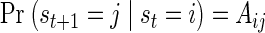
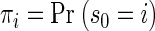
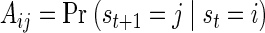
In the HMM, epochs of neural activity are explicitly represented by the value of a latent state variable, s_t, whose change in time is modeled as a first-order Markov process. This implies that the probability of transition from state i to state j at time t + 1, A_ij, depends only on the state at time t

(1)

State changes and neural activity are considered in 10-ms time steps. The Markov assumption enables the information gleaned from the neural activity in one 10-ms period to be appropriately combined with information from all previous periods of activity in an efficient recursive manner amenable to real-time processing. We will denote the number of spikes recorded in a 10-ms window following time t by n_t(k) for the kth neuron in the ensemble. Furthermore, the activity of the ensemble of N neurons is denoted by the column vector n_t = [n_t(1) n_t(2)… n_t(N)]^T.

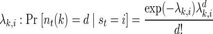
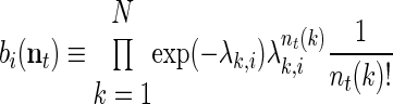
In addition to a model of state transitions, an HMM is specified by the way the latent state variable can be observed. Conditioned on the state of the system, we modeled spikes as a Poisson process with a constant firing rate. The conditional probability of observing d spikes from neuron k is thus

(2)

where λ_ki, is the mean firing rate of neuron k when the state of the underlying process at time t, s_t, is i.

Notice that the choice of a Poisson model of activity implies the assumption that, conditioned on being in a particular state, the activity of each neuron observed will be temporally homogeneous (the same rate across trials). To account for the obvious dependence of ensemble firing rates on the intended target of movement, we used a model with separate states for each target during each directional epoch (one plan and one perimovement state per target). Furthermore, the firing rates of neurons in the ensemble are highly variable during the baseline epoch. To account for this variability, we used five separate states during baseline (similar performance was observed for three to eight baseline states). Figure 2A depicts this simple HMM, with each circle representing an HMM state and single arrows representing allowed state transitions. Corresponding to each state is a different vector of firing rates. Note that this form of representation is distinct from a “graphical model,” an alternative graphical format that depicts the probabilistic relationship between latent states and between latent states and observations.

FIG. 2.

We model observed neural activity as the output of the depicted first-order hidden Markov process. Circles represent hidden states (each corresponding to a different vector of neural firing rates) and single arrows represent allowed state transitions. A: in our simple hidden Markov model (HMM), there are 2 states for each reach goal. The double arrows represent the full interconnectedness of the baseline states, and that they are fully connected to the preparatory states. B: in the extended HMM, there are multiple states for each reach goal, but they are connected in a left-to-right manner: transitions occur only from one state to the next.

For the stereotyped center-out movements generated by a trained subject, the patterns of neural activity are highly similar. As a result it is possible to model the temporally inhomogeneous patterns of neural activity accompanying the preparation and execution of movement to a particular target with a single pair of states. However, to test the importance of representing temporal variability in neural activity, in addition to the simple, two-state-per-target HMM, we created a second, extended HMM. In the extended HMM, plan and perimovement activity for movements to a particular target are modeled as a series of connected states, as depicted in Fig. 2B. For both models, we specified the state transition matrix A, such that transitions were permitted between all baseline states, from each baseline state into the first of each target-dependent state sequence and then in a left-to-right manner between target-dependent states, as shown by the arrows in Fig. 2.

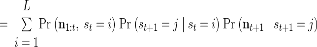
The a posteriori likelihood (APL) of a state j, at time t, Pr (s_t = j|n_0:t), is a measure of the probability that the observed neural activity from time 0 to time t arose from a sequence of states that concluded in state j at time t. Notice that, although the model prohibits transitions from states corresponding to one target to states corresponding to another, the APL of states corresponding to different goals may display large fluctuations, initially suggesting one goal is most likely, then, after neural activity accumulates, shifting to strongly indicate a different goal.

The APL can be calculated recursively

(3)

where L is the total number of states in the HMM and π_j ≡ Pr (s₀ = j). The recursive multiplication of many probabilities results in numbers that quickly converge to zero. Thus when calculating the APL, we normalize the probability at each time step to guard against numerical underflow. Details of our specific implementation are given in the appendix.

The didactic model in Fig. 3 was trained using only 10 neurons and reaches to only two targets. Figure 3B depicts the activity of these neurons in an example test trial. Figure 3C depicts the estimated APL for this trial. In this example, the transitions from baseline to preparatory to perimovement regimes of activity are quite apparent in the spikes and, as expected, the estimated state likelihoods track these transitions quite accurately and closely.

FIG. 3.

A: simple 5-state reaching-movement HMM. The neural activity transitions from a baseline state to one of 2 possible planning states. After some period of planning, the activity transitions to a perimovement state. During any small period of time, the actual state itself is not directly observed. Rather, individual neurons change their firing rates depending on the state. B: an example of the neural activity for a rightward movement. C: on an individual trial, the a posteriori likelihood of each of the states given all the data received up to the current time can be calculated. The result is a time series of state likelihoods as shown. By evaluating when and which state likelihoods cross a threshold, we can estimate the state of the neural activity (e.g., baseline, planning, or moving) and the target of the movement. The arrow depicts the estimated time of the beginning of the planning regime for the threshold value depicted.

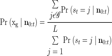
We use the APL for both epoch detection and target estimation. To determine the current epoch of activity, the APL is combined across goals. For the plan epoch

(4)

where 𝒫 represents all plan states for all target locations. Equivalently, we can find the APL of perimovement states. Then, the time at which this APL crosses a predetermined threshold is an estimate of the moment of transition between activity regimes. Shown in Fig. 3C is a 90% probability threshold and the corresponding moment at which the transition to preparatory activity is detected. Note that higher threshold values result in fewer false-positive epoch detections but longer latencies between target onset and epoch detection; an operational system would choose a threshold value based on user preferences. We considered using ML simultaneously for both epoch and target estimation. However, we discovered that during the periods of transition from one epoch to another, there were sometimes brief elevations in the APL corresponding to targets other than the one finally converged on. Thus by combining across targets, we were able to estimate the moment of epoch transition before the APL of a state corresponding to a particular target had stabilized.

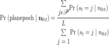
Following epoch detection, we further use the APL for target estimation, combining likelihoods of states corresponding to the same target. For a particular target, x_g, we have

(5)

where 𝒢 represents the states corresponding to target x_g. Our estimate is then the target that maximizes Pr (x_g|n_0:t). As depicted in Fig. 3C, this is typically simply equivalent to the target corresponding to the ML state. As follows from our description of the initial instability of the APL corresponding to individual targets, we found that target estimation could be improved by waiting a fixed period following epoch detection, integrating additional neural activity into the APL prior to decoding. This delay results in a further trade-off of latency and accuracy, which can be optimized per user preference.

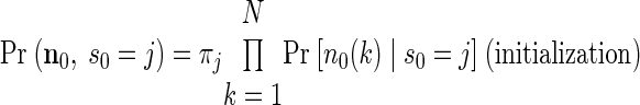
The primary contrast between this work and previous applications of HMMs to neural activity (Abeles et al. 1995; Hudson and Burdick 2007; Seidemann et al. 1996) is in the approach taken to learn the HMM parameters. Rather than attempting to learn the state-dependent structure of the neural activity in an unsupervised way, we assumed the availability of training data with rough epoch boundaries. This allowed us to learn the parameters of our HMM—the state transition matrix, the state-conditioned firing rates, and initial state probabilities—using expectation maximization (EM). The EM algorithm is a general iterative approach for finding the parameters in models like the HMM. A good tutorial is that of Rabiner (1989); the specific equations used in this work are given in the appendix. Specifically, we used a training data set consisting of 50 reaches to each of the eight targets. Hidden Markov model parameter learning using EM is often sensitive to the values used in initialization. In the unsupervised learning case, in which the desired structure of the final model is highly uncertain, a variety of strategies can be used to decrease this sensitivity (Abeles et al. 1995; Seidemann et al. 1996) or different learning approaches can be used (Hudson and Burdick 2007). In our case, the desired model structure was known and learning was used primarily to fine-tune parameters.

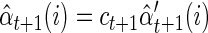
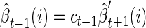
We created an initial model with the desired characteristics by specifying an appropriate state transition matrix and initializing state firing rates to correspond to the mean firing rates in the appropriate periods (baseline: prior to and immediately after target onset; plan: following target onset; perimovement: following the go cue). State transition probabilities from the eight preparatory states were set to 0.9 and 0.1, respectively, for the probability of return and the probability of transition to the corresponding perimovement state. Perimovement states are absorbing (the probability of transition to any other state is equal to zero). The probabilities of transitions between the five fully connected baseline states and from each baseline state to each preparatory state are set to be equal. The initial probabilities of the preparatory and perimovement states were zero and the initial probabilities of the five baseline states were equal.

The specific periods of neural activity used to initialize the model firing rates are specified in Table 1. In the simple HMM, the mean ensemble firing rates in each period were calculated from the 50 training trials for each target and assigned to the appropriate state. In the extended HMM, the plan and perimovement periods were subdivided respectively into 10 and 25 equally sized windows and the average activity in each window was used for state initialization. The baseline activity period was split into five windows and the mean firing rates over all training trials were assigned to the five baseline states. Note that performance is not sensitive to the exact number of states chosen for the various epochs.

TABLE 1.

Parameter initialization

State	Period	Simple HMM	Extended HMM
Baseline	[tTARGET − 200 ms : tTARGET + 150 ms]	5 consecutive states
Plan	[tTARGET + 150 ms : tTARGET + 750 ms]	1 state	10 consecutive states
Perimovement	[tVELMAX − 250 ms : tVELMAX + 350 ms]	1 state	25 consecutive states

For limited training data, the large number of states in the extended HMM render it vulnerable to both misfitting and overfitting. To ensure that the model we desired was the one actually learned, we generated appropriate initial conditions by first running EM for each target separately—on only the baseline states and the states corresponding to that particular target. Then, these submodels were combined and EM was run on the complete extended HMM, with a convergence threshold chosen to avoid overfitting.

Real-time implementation

The causal design of our simple and extended HMM algorithms makes them easily amenable to a recursive real-time implementation. However, it is unclear how much computational delay the real-time implementation would introduce in addition to the latency caused by the algorithm itself. This is delay in association with epoch and target estimation as well as the length of time required to render the appropriate icon to the monkey (termed T_dec+rend in Santhanam et al. 2006).

To show that it is possible to create an implementation that does not result in additional delay that would impede usability, we extended our experimental platform to allow for real-time epoch and target estimation. This required performing real-time spike sorting and neural data collection as described in Santhanam et al. (2006). In addition, two other computers were used: one to extract the relevant window of neural activity at submillisecond resolution (30-kHz sampling with Pentium 4, 2.8 GHz), another to calculate all of the relevant state probabilities and report a decoded target when appropriate (AMD Athlon dual-core, 2.2 GHz). All of the machines that handled raw neural data from the amplifier were running real-time Linux, which allowed for the real-time hardware control necessary for the precise timing required; the machines that dealt with stimuli presentation were running Windows and DOS. Our implementation fetched 50-ms blocks of neural data at a time to allow for latencies involved in packaging the spiking data into Matlab structures. Spikes were binned every 10 ms as described earlier.

Our real-time system was tested on neural data while monkey H was performing arm movements. The extended HMM was used with 10 planning states and 45 movement states for each target and 5 baseline states. The probability of the plan epoch was defined as the sum of being in the latter 9 of 10 plan states. The implementation latency was therefore the difference in time between when the probability of the plan epoch exceeded threshold and the time that the decoded icon was displayed to the monkey. This was measured to be about 30–40 ms, which is about the same as that reported in Santhanam et al. (2006) for our fixed-paced decoder. Thus even though the extended HMM requires more computations than simple maximum likelihood, the computational difference is not great enough to result in a noticeable delay when implemented in real time.

RESULTS

The task of decoding movement intent from preparatory neural activity for a neural prosthesis motivated us to develop an HMM-based algorithm that could detect the transitions in ensemble activity between baseline, planning, and execution of movements. Following detection of the plan epoch, the intended target of movement is then decoded. The final performance of the neural prosthesis will thus depend on two aspects of the system: how reliably the epoch of plan activity can be detected and how accurately the intended target can be decoded from plan activity.

In the absence of errant HMM behavior, the neural activity should transition from the baseline to the plan epoch at some point following the target onset. Thus detection of this transition is characterized by a latency relative to target onset and jitter, the trial-to-trial variability in this latency. As described earlier, larger thresholds result in increased latency. Figure 4A shows cumulative distributions of the latency for three different values of the threshold. However, whereas larger thresholds on average lead to increasing latency, as shown in Fig. 4B, they also lead to decreased jitter (defined as the SD of the latency across the test trials). However, as the threshold gets too close to one, as shown in the top panel of Fig. 4B, the number of trials in which the likelihood of the plan epoch never exceeds threshold increases, and thus the jitter and latency (calculated excluding trials in which the plan epoch is never detected) begin to rise precipitously. Given the internal nature of the transition from baseline to plan epochs, we have no independent measure of its variability. On the other hand, we can directly observe the reaction time of the subject to the go cue using a hand velocity threshold (0.025 m/s threshold; mean velocity 100 ms prior to go cue was 0.003 and 0.004 m/s for G and H, respectively). This variation, shown by the gray line in Fig. 4B, provides a lower bound to the jitter of the neural reaction to the go cue and, if epoch transitions follow similar timelines, a lower bound to the jitter in the transition from baseline to plan epochs.

FIG. 4.

The HMM detects a transition to the plan epoch with some latency following the appearance of the target. A: cumulative distributions of the detection latency for 3 values of the threshold (0.5, solid; 0.9, dashed; and 0.999, dotted). Note how the center of the distribution shifts rightward (later) with increasing threshold values. Furthermore, low values of threshold result in a large fraction of premature epoch predictions, seen as nonzero values at zero latency. B: the mean latency (solid black line) increases with increasing threshold. The jitter, or SD of the latency, first decreases then increases with increasing threshold (dashed line). For comparison purposes, the SD of the subject's behavioral reaction times to the go cue is shown in gray. Top and bottom panels present data from monkeys G and H, respectively.

Figure 4 depicts that for smaller values of the threshold, it is more common to misestimate the time of transition-to-plan too early than too late. We wondered whether this might be a result of modeling the neural firing in the plan epoch with only one state per target. Thus we implemented an extended HMM model with 10 states modeling the time course of plan activity. Figure 5 compares the distribution of epoch detection times estimated using the extended HMM with those of the simple HMM. In general, the extra states provided in the extended HMM resulted in earlier epoch detection. Additionally, however, the shorter latency was accompanied by a smaller jitter, as would be expected if the extra states improve our model of neural activity. In training, the plan states of the extended HMM were initialized with data 150 ms following target onset. Figure 5B suggests that the EM algorithm learns to assign neural activity preceding this moment to the plan states. This points out a significant advantage of the HMM approach: accurate knowledge of the specific timing of transitions on a trial-by-trial basis is not required for model parameter estimation.

FIG. 5.

The extended HMM represents an intended movement to a given target with several states. The onset of the plan epoch is detected by collapsing the likelihood across all the appropriate states. A: comparison of the distribution of epoch detection latency generated by the extended HMM (black lines) with that of the simple HMM shown in Fig. 4 (gray lines) using the same 3 values of threshold (0.5, solid; 0.9, dashed; 0.999, dotted). B: comparison of the mean latency (solid lines) and jitter (dashed lines) as a function of increasing threshold, extended HMM (black lines), and simple HMM (gray lines). Top and bottom panels present data from monkeys G and H, respectively.

For the neural prosthetic decoder application, detection of the onset of the plan epoch is used to enable a second stage of decoding—i.e., target estimation. An approximation of the upper limit of target estimation accuracy (fraction of targets correctly decoded) is the ML approach, with known epoch timing presented in Santhanam et al. (2006), using a 200-ms neural activity window beginning 150 ms following target onset. Over the test trials, the application of this approach yielded a mean accuracy of 91% (89%) for monkey G (H). Recall that the choice of HMM decoder parameters results in a trade-off of latency and accuracy. The solid line in Fig. 6 compares the accuracy of HMM-based decoding following the detection of the plan epoch with the latency of detection for increasing values of the epoch detection threshold. The peak detection accuracy, 86% (81%), occurs with a mean latency of 292 ms (321 ms). Note that trials in which detection of the plan epoch occurred >700 ms following target onset are considered failures, lowering the accuracy and not contributing to the mean latency. Thus for the HMM, epoch detection results in a loss of about 5–10% in accuracy relative to known epoch timing.

FIG. 6.

Increasing the plan epoch detection threshold leads to both an increase in the latency of detection relative to target onset and an increase in the accuracy of the estimated intended target of movement in the simple HMM. The solid line shows the accuracy as a function of the average latency for increasing threshold values; 0.9 to 1 × 10⁻⁶ (left) and 0.9 to 1 × 10⁻⁹ (right). The likelihood of the plan epoch converges faster than the likelihood of the particular target, thus delaying target estimation until 100 ms (dashed line) or 200 ms (dotted line); following the detection of the plan epoch can further increase decoding accuracy. With this added delay, HMM-based decoding approaches the accuracy of maximum likelihood (ML) when the time of target onset is known to the decoder (depicted as a cross). Left and right panels depict results for monkeys G and H, respectively.

We suspected that the likelihood of the plan epoch might converge faster than the likelihood of the proper target. Thus we also calculated the ML target at various delays following the detection of the plan epoch. This allowed the HMM to accumulate additional neural activity into the state likelihoods and thus would presumably increase the accuracy of the detected target at the cost of increased latency. The dotted and dashed lines in Fig. 6 depict decoding accuracy as a function of latency when an additional 100 or 200 ms of neural activity is accumulated following the detection of the plan epoch prior to target decoding. With a lower threshold and an additional 100 ms of neural activity, the HMM can achieve 89% (85%) accuracy with a latency of 328 ms (332 ms). For comparison, our previously reported FSM method has one parameter—the number of consecutive plan epoch detections (C_plan), which has a similar effect to trade-off latency and accuracy. For C_plan of 20 (optimized for highest accuracy with latency <350 ms), the accuracy of the FSM is 84% (83%) with an average latency of 333 ms (344 ms).

The extended HMM represents the time course of the plan activity epoch in multiple states. As described earlier, one result of these extra states is that the plan epoch is actually often detected earlier than expected. This is primarily because of predicted early transitions to the first of the plan epoch states corresponding to one of the intended targets. Not surprisingly, we found that if we excluded the first plan state from the epoch detection likelihood, we delayed detection. This is equivalent to forcing the HMM to ignore the neural activity representing the early transient response to the target onset. Knowing that other algorithms showed increased accuracy when neural activity >150 ms following target onset was considered, we expected that target estimation would be more accurate if the first plan state was excluded from both the epoch detection and target estimation process. As shown in Fig. 7A, not only is this the case, but excluding even more of the initial states further improves decoding accuracy at the cost of increased latency. Table 2 summarizes the optimized accuracy of the windowed ML, FSM, simple HMM, and extended HMM decoding algorithms.

FIG. 7.

Increasing the detection threshold results in increased latency of detection and increased accuracy for the extended HMM. The solid line depicts the trade-off of mean latency and accuracy for values of threshold from 0.5 to 1 × 10⁻⁸. In the extended HMM, excluding the first of each target's plan epoch states from the likelihood calculation further increases the latency of epoch detection, of which the earliest plan-related neural activity modeled by each of these states was ignored. However, the increased latency is accompanied by increased accuracy. As the value of the threshold increases even further, however, accuracy decreases as the likelihood fails to cross threshold within 700 ms in some trials. The dashed line depicts the latency–accuracy trade-off for increasing threshold when the plan epoch likelihood is calculated using only the latter 9 states per target. The dotted line depicts the trade-off when only 8 states per target are used. Note that performance equals or exceeds the known-timing ML accuracy depicted by the cross. Left and right panels depict results for monkeys G and H, respectively.

TABLE 2.

Algorithm performance comparison

Algorithm	Accuracy, % Monkey G (H)	Latency, ms	Parameters
Windowed ML (Known epoch)	91 (89)	350 (350)	Window = 150–350 ms following target onset
FSM (Achtman et al., unpublished)	85 (83)	348 (334)	Cplan = 14 (20)
HMM	90 (85)	339 (342)	Delay = 140 ms (100 ms), Threshold = 1–1e-4 (1–1e-8)
Extended HMM	94 (90)	340 (332)	Plan epoch states = 4–10 (4–10), Threshold = 0.9 (0.7)

Model robustness

We have demonstrated that an HMM can be used to simultaneously detect the onset of neural activity related to an intended movement and decode to which of several targets the user desires to move. However, the HMM presented earlier required modeling the neural activity to each possible desired target. We investigated whether a simple HMM could additionally detect the onset of neural activity related to movements that were not explicitly modeled. To test this question, we trained a simple HMM using trials corresponding to reaches to only four of the eight targets in our data set (70, 150, 230, and 350°). Using this model, we evaluated whether we could accurately detect the transition to the plan epoch in the neural activity corresponding to movements to the other four targets. Figure 8 depicts a cumulative distribution of the detected transition times, comparing test trials corresponding to trained targets with those corresponding to novel targets. In general, transitions for novel targets were slightly later than those for the trained targets, but were still readily detected. Interestingly, on trials to novel targets, the decoded target is the target adjacent to the novel one in 99% of trials for both monkeys. This suggests that the HMM is able to detect similarities in the pattern of activity for similar movements. Thus it appears that a simple HMM can be useful for detecting transitions in neural activity, even when the movements involved differ from those modeled in training.

FIG. 8.

The simple HMM was trained using data corresponding to only 4 of the 8 reach targets. The cumulative distribution of the latency of detection of the plan epoch for a threshold of 0.99 is depicted. The black line represents the cumulative distribution of epoch detection latency for test trials to the 4 targets used for training. The gray line represents the cumulative distribution of latency for test trials to the other 4 novel targets. Although there is a slight increase in latency, the plan epoch appears to be easily detected in the case of the novel targets. Left and right panels depict results for monkeys G and H, respectively.

Perimovement activity

In addition to plan activity, our HMM included states representing the neural activity that accompanies the actual execution of the center-out reaches in our task. Although it was possible to replicate the preceding results using the movement epoch rather than the plan epoch, our interest in the communications prosthetic application led us to focus on plan activity. However, in cases in which the microelectrode array is implanted in areas with well-tuned perimovement activity, its use may be desirable. Optimized results when the ML target is estimated immediately following the detection of the movement epoch are given in Table 3. The latency of perimovement activity is measured relative to target onset. The mean and SD (jitter) of the behavioral reaction times, also measured relative to target onset, are given for comparison purposes. Both simple and extended HMMs detect a transition to the movement epoch about 150 ms following the go cue. The beginning of the physical movement occurs about 100 ms later. From the standpoint of a neural prosthetic interface, this intriguing result suggests that the prosthetic device could initiate movement at the same rate as normal or perhaps even faster!

TABLE 3.

Decoding using perimovement activity

Algorithm	Accuracy, %	Mean Latency, ms (Jitter, ms)	Threshold	Mean RT, ms (Jitter, ms)
HMM
G	98	164 (114)	1–1e-8	244 (21)
H	98	160 (114)	1–1e-10	253 (21)
Extended HMM
G	98	125 (83)	1–1e-6	244 (21)
H	99	137 (81)	1–1e-6	253 (21)

DISCUSSIONS

In prior neural prostheses, when different epochs of neural activity have been taken into account, the boundaries of these epochs have been typically specified by the experimenter. This work builds on Achtman et al. (unpublished data) by developing a rigorous two-phase decoding system in which the epoch of neural activity is first detected, then the appropriate model is applied to decode the intended target of movement. The HMM approach allows baseline, plan, and perimovement epochs of neural activity to be represented by series of unobserved states coupled to a Poisson model of activity. In explicitly modeling epochs of neural activity, this work contrasts quite significantly from previous uses of HMMs to model cortical activity (Abeles et al. 1995; Seidemann et al. 1996), in which hidden states were used to represent patterns for which no a priori hypothesis of the actual temporal structure could be made. In our work, we begin with the assumption that there are three epochs of neural activity that our model should represent and, for training, we can segment our data using known temporal markers such as experimental cues and behavioral data.

Compared with our simplest HMM, we found that using the extended HMM for target decoding typically resulted in an increase in accuracy of about 5%, allowing the performance of our decoder to meet or exceed the level of known-timing ML. This additional performance suggests that taking into account the temporal characteristics of the patterns of neural activity may be important for a good epoch detector. An alternate approach would be to use a mixture of models of neural activity with continuous valued state, such as in Yu et al. (2006), for the various epochs coupled to a discrete latent variable representing the epoch. Unfortunately, the training and decoding for these types of models lack the simple closed forms of the HMM. Similarly, we represented movement intention and execution as being an uninterrupted process. In reality, users might abort their intent or change their intended targets during the plan epoch. Although a fully connected state transition matrix would accommodate these sorts of dynamics, accurate model learning would likely require significantly more trials.

In general, the amount of neural activity detectable by a chronically implanted cortical microelectrode array is initially quite limited and decreases with time. As a result of this limited information, there is a fundamental trade-off between the flexibility (the range of potential movements) and accuracy of a neural prosthesis interface. On the basis of this limited information, we chose to operate in a regime of higher reliability but lower flexibility—the regime of a fixed number of discrete targets. Despite this choice, our activity-segmenting algorithm appears to work even in the case of novel targets, and thus there is potential to improve other existing systems merely by coupling them with our algorithm. For example, most existing continuous prosthesis decoding systems do not specifically detect when movements should be made. Instead, an external operator enables them during movement; thus the performance of this type of system during nonmovement periods has yet to be quantified. Whether these current decoders incur high error during nonmovement periods has yet to be quantified. If these current decoders incur high error during nonmovement periods, as our experience suggests, our HMM-based scheme could be used as a high level controller, passing control to the continuous decoder only when perimovement activity is detected.

We have shown previously (Kemere et al. 2004b) that for stereotyped movements, a model of canonical trajectories can be coupled to an estimate of the intended target of movement to generate a decoded trajectory. In addition, we have also shown that an estimate of the target of movement generated from plan activity can be used to improve the accuracy of a trajectory decoded from perimovement activity (Kemere and Meng 2005; Kemere et al. 2004a; Yu et al. 2007). An epoch detector, such as that presented in this work, is required for systems that seek to realize this performance increase.

We used the accuracy of the ensuing decoding to judge the optimality of an epoch-detection threshold. An alternate approach would be to minimize latency while also minimizing the number of premature or very late epoch detections, which might correspond to finding the threshold level that minimized the jitter or some other measure of the tightness of the epoch-detection distribution. Interestingly, the minimum jitter we were able to detect in transitions in neural activity, about 70 ms, is still much larger than the 20-ms jitter observed in behavioral reaction times. Although this may merely be evidence of suboptimality of our algorithm or an insufficiency of neural data, it may also reflect something real in the neural activity—that is, a greater variation in the length of time the neural activity takes to converge from an unspecific baseline to an appropriate plan for a particular target (Churchland et al. 2006b).

As discussed earlier, we have recently implemented this algorithm in real time. Although a detailed discussion of the performance achieved is outside the scope of this report, this demonstration underscores the point that such a system is indeed realizable. Further, our platform is easily extensible to allow for integration of other algorithms, such as mixture models that decode trajectories (Yu et al. 2007) or other epoch and target estimation algorithms. Of course, natural movements lacking some of the somewhat artificial characteristics of our reaching task—enforced eye fixation and delay between target onset and the go cue—may result in patterns of activity that would potentially be more difficult to decode. Furthermore, the HMM approach might have difficulty with indecisive or distracted movements, uncommon in our paradigm but potentially a factor for functioning prostheses. A fully autonomous neural prosthesis would additionally require the ability to make a series of movements without external triggering. We could have implemented this feature by adding state transitions from the perimovement states back to baseline. Alternatively, the system could automatically return to the baseline state following the selection of a target. Our segmented data set did not permit us to compare the performance of either of these approaches.

Finally, the HMM-based approach to finding transitions in neural activity between different epochs of activity may have utility beyond neural prosthesis interfaces. Prior work with these models (Abeles et al. 1995) has, in fact, focused on data in which neural activity was thought to oscillate between unobservable states. The desire to study problems in which trial-by-trial evaluations of mental states are of interest (Yu et al. 2006) will increase with increasing adoption of dense multielectrode neural recordings. The technique we developed in this work—using known trial parameters to ensure that the hidden states of the HMM represent interpretable regimes—should serve as a guide to investigators hoping to use these techniques in the future.

GRANTS

This work was supported by a Center for Circuit & System Solutions/MARCO Focus Center Research Program grant to C. Kemere and T. H. Meng, National Defense Science and Engineering Graduate Fellowships to G. Santhanam and B. M. Yu, National Science Foundation Graduate Fellowships to G. Santhanam and B. M. Yu, a Christopher Reeve Paralysis Foundation grant to S. I. Ryu and K. V. Shenoy, a Stanford University Bio-X Fellowship to A. Afshar, a Stanford–National Institutes of Health Medical Scientist Training Program grant to A. Afshar; and the following awards to K. V. Shenoy: the Burroughs Wellcome Fund Career Award in the Biomedical Sciences, the Center for Integrated Systems at Stanford, the Office of Naval Research (Adaptive Neural Systems), the Sloan Foundation, and the Whitaker Foundation.

APPENDIX: PARAMETER ESTIMATION FOR HMM

For this work, we use an iterative expectation–maximization (EM) algorithm (Baum et al. 1970; Dempster et al. 1977; Rabiner 1989) to estimate the parameters of our HMMs. Our HMM is described by three parameters: θ = {π, A, λ}

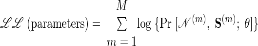
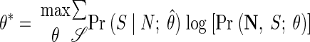
For trial m, assume S^(m) is the sequence of states that gave rise to the neural activity, 𝒩^(m) = n_0:Tm. Thus for the M trials in our training data, we would like to find the parameters θ = θ*, which maximize the log-likelihood

However, because we cannot observe S^(m) directly, we approximate using our observations

Since we also lack perfect knowledge of the parameters, θ, we iterate, using the current estimate of the parameters θ̂ to calculate E{log [Pr (N, S; θ)]|N; θ̂}, then finding the value of θ = θ* that maximizes the expectation and repeating with θ̂ = θ*. It has been shown (Baum et al. 1970; Dempster et al. 1977) that this iteration results in increasing likelihoods, reaching a unique maximum if it exists.

Thus each iteration of the EM algorithm involves two steps: 1) the “expectation” (E) step, that is, computing the expected log-likelihood function; and 2) the “maximization” (M) step; that is, find the value of the parameters, θ*, that maximize it. This appendix describes the EM algorithm applied to our particular HMM.

Expectation

The first step of the EM iteration is the E step. The goal of this step is to efficiently calculate for all states i and j

(A1)

and

(A2)

respectively the probability of being in state i at time t and the probability of being in state i at time t and state j at time (t + 1). Importantly, notice that in both cases, these probabilities are conditioned on all the neural activity (n_0:T) from a particular trial. We can calculate these densities efficiently with only two passes through the data using the “Forward–Backward” algorithm. At each point in time, we combine information received from time 0 forward to the present [the forward density, α_t(i) ≡ Pr (n_1:t, s_t = i)] with information received from time T back to the present [the backward density, β_t(i) ≡ Pr (n_t+1:T, s_t = i)]. The product of the forward and backward densities at time t is simply Pr (n_0:T, s_t = i), which is proportional to the expression in Eq. A1.

We define the state-dependent observation function for state i

A recursive calculation is used for the forward density

and the backward density

As mentioned in the text, implementing the forward–backward recursions as written would quickly result in numerical underflow (all numbers tending toward zero). Thus it is critical to rescale at each step. For the forward density, we simply normalize the values to sum to one

As described in Rabiner (1989), it is convenient to use the same scaling factor for the reverse density

Notice that, because of the normalization at each step, it is not necessary to include the factorial term in the observation density b_j(n_t) because it is common to all states. Additionally, to prevent large fluctuations when a spike is observed from a neuron whose firing rate is very low, we enforce a minimum firing rate of 1 Hz.

Maximization

In the M step, we find the model parameters that best fit the latent state probabilities calculated in the E step. Specifically, we wish to find the parameters θ*

(A3)

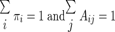
Note that the sum is taken over all possible state sequences and that Pr (𝒮|N; θ̂) is calculated during the E step. Furthermore, the initial state probabilities, π_i, and state transition probabilities, A_ij, must be found subject to the constraints

The maximizing values for the initial probabilities and state transitions (Rabiner 1989) are

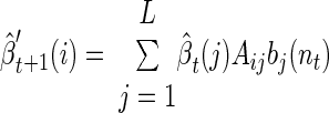
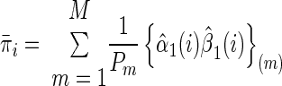and

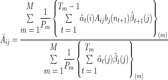For the Poisson firing rates, the formula is

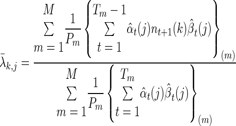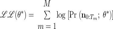
To determine model convergence, we use the log-likelihood of the parameters, the log of the a posteriori probability of the entire training data, ℒℒ(θ*) = ∏_m=1^M Pr [(n_0:Tm)_(m); θ*]. Notice that this can be calculated using the forward density or the scaled forward density, as shown in Rabiner (1989)

We specified a criterion on the proportional change in this log-likelihood: (new − original)/original: 10⁻³ for the simple HMM and for the submodel training in the extended HMM, and 10⁻¹ for the primary training of the extended HMM.

In the case of the simple HMM, the proportional change in the log-likelihood dropped to <10⁻³ after 1–2 iterations of EM, 10⁻⁴ after about 10 iterations, and 10⁻⁶ after about 30 iterations. The rate of convergence depended on the number of baseline states; for a simpler model with only one baseline state, the proportional change reached 10⁻¹⁰ within 7 iterations of the EM algorithm. However, extending learning beyond the first 1–2 iterations had little effect on the subsequent detection or decoding. To test the effect of learning on model parameters, we generated a simulated data set. We generated Poisson random firing, where the firing rates were generated from averages of our experimental data. We also used the trial timing of our training data set to specify when the simulated neural activity should switch between the three epochs (with the actual transition happening 100 ms following the target onset and go cue). Using the same training initialization and learning procedure, we then evaluated convergence of the HMM using 50 different simulated data sets. We found that log-likelihood convergenced quickly, similar to the actual training data. Furthermore, we examined how the learned firing rates changed from one iteration to another. We found that the mean-square difference between EM-learned firing rates and those used to generate the simulated data converged at about the same rate, reaching a final (but of course nonzero) value within 1–2 iterations. Because neither our simulation nor the actual data actually arise from a Markov process, we did not evaluate the convergence of the state transition matrix. Thus for the HMMs used in this work, in which the state-dependent firing of the neurons can be closely initialized using training data, a few iterations of the EM algorithm suffice to achieve a converged model.

REFERENCES

- Abeles 1995.Abeles M, Bergman H, Gat I, Meilijson I, Seidemann E, Tishby N, Vaadia E. Cortical activity flips among quasi-stationary states. Proc Natl Acad Sci USA 92: 8616–8620, 1995. [DOI] [PMC free article] [PubMed] [Google Scholar]
- Achtman 2007.Achtman N, Atshar A, Santhanam G, Yu BM, Ryu SI, Shenoy KV. Free-paced high-performance brain-computer interfaces. J Neural Eng 4: 336–347, 2007. [DOI] [PubMed] [Google Scholar]
- Baum 1970.Baum LE, Petrie T, Soules G, Weiss N. A maximization technique occurring in the statistical analysis of probabilistic functions of Markov chains. Ann Math Stat 41: 164–171, 1970. [Google Scholar]
- Carmena 2003.Carmena J, Lebedev M, Crist RE, O'Doherty JE, Santucci DM, Dimitrov D, Patil P, Henriquez CS, Nicolelis MA. Learning to control a brain-machine interface for reaching and grasping by primates. PLoS Biol 1: 193–208, 2003. [DOI] [PMC free article] [PubMed] [Google Scholar]
- Churchland 2006a.Churchland MM, Santhanam G, Shenoy KV. Preparatory activity in premotor and motor cortex reflects the speed of the upcoming reach. J Neurophysiol 96: 3130–3146, 2006a. [DOI] [PubMed] [Google Scholar]
- Churchland 2006b.Churchland MM, Yu BM, Ryu SI, Santhanam G, Shenoy KV. Neural variability in premotor cortex provides a signature of motor preparation. J Neurosci 26: 3697–3712, 2006b. [DOI] [PMC free article] [PubMed] [Google Scholar]
- Crammond 2000.Crammond DJ, Kalaska JF. Prior information in motor and premotor cortex: activity during the delay period and effect on premovement activity. J Neurophysiol 84: 986–1005, 2000. [DOI] [PubMed] [Google Scholar]
- Danóczy 2006.Danóczy M, Hahnloser R. Efficient estimation of hidden state dynamics from spike trains. In: Advances in Neural Information Processing Systems, edited by Weiss Y, Schölkopf B, Platt J. Cambridge, MA: MIT Press, 2006, vol. 18, p. 227–234.
- Dempster 1977.Dempster A, Laird N, Rubin D. Maximum likelihood from incomplete data via the EM algorithm. J R Stat Soc B Method 39: 1–38, 1977. [Google Scholar]
- Deppisch 1994.Deppisch J, Pawelzik K, Geisel T. Uncovering the synchronization dynamics from correlated neuronal activity quantifies assembly formation. Biol Cybern 71: 387–399, 1994. [DOI] [PubMed] [Google Scholar]
- Donoghue 2002.Donoghue JP Connecting cortex to machines: recent advances in brain interfaces. Nat Neurosci Suppl 5: 1085–1088, 2002. [DOI] [PubMed] [Google Scholar]
- Fetz 1999.Fetz EE Real-time control of a robotic arm by neuronal ensembles [Comment]. Nat Neurosci 2: 583–584, 1999. [DOI] [PubMed] [Google Scholar]
- Georgopoulos 1982.Georgopoulos AP, Kalaska JF, Caminiti R, Massey JT. On the relations between the direction of two-dimensional arm movements and cell discharge in primate motor cortex. J Neurosci 2: 1527–1537, 1982. [DOI] [PMC free article] [PubMed] [Google Scholar]
- Hochberg 2006.Hochberg LR, Serruya MD, Friehs GM, Mukand JA, Saleh M, Caplan AH, Branner A, Chen D, Penn RD, Donoghue JP. Neuronal ensemble control of prosthetic devices by a human with tetraplegia. Nature 442: 164–171, 2006. [DOI] [PubMed] [Google Scholar]
- Hudson 2007.Hudson N, Burdick J. Learning hybrid system models for supervisory decoding of discrete state, with applications to the parietal reach region. In: Proceedings of the 2007 CNE'07 3rd International IEEE/EMBS Conference on Neural Engineering. Piscataway, NJ: IEEE, 2007, p. 587–592.
- Kemere 2005.Kemere C, Meng TH. Optimal estimation of feed-forward-controlled linear systems. In: Proceedings of the IEEE International Conference on Acoustics, Speech, and Signal Processing, Philadelphia, PA. Piscataway, NJ: IEEE, 2005, vol. 5, p. 353–356.
- Kemere 2004a.Kemere C, Santhanam G, Yu BM, Ryu SI, Meng TH, Shenoy KV. Model-based decoding of reaching movements for prosthetic systems. In: Proceedings of the 26th Annual Conference of the IEEE/EMBS, San Francisco, CA. Piscataway, NJ: IEEE, 2004a, p. 4524–4528. [DOI] [PubMed]
- Kemere 2004b.Kemere C, Shenoy KV, Meng TH. Model-based neural decoding of reaching movements: a maximum likelihood approach. IEEE Trans Biomed Eng 51: 925–932, 2004b. [DOI] [PubMed] [Google Scholar]
- Kennedy 1998.Kennedy PR, Bakay RA. Restoration of neural output from a paralyzed patient by a direct brain connection. Neuroreport 9: 1707–1711, 1998. [DOI] [PubMed] [Google Scholar]
- Kennedy 2000.Kennedy PR, Bakay RA, Moore MM, Adams K, Goldwaithe J. Direct control of a computer from the human central nervous system. IEEE Trans Rehabil Eng 8: 198–202, 2000. [DOI] [PubMed] [Google Scholar]
- Kipke 2003.Kipke DR, Vetter RJ, Williams JC, Hetke JF. Silicon-substrate intracortical micro-electrode arrays for long-term recording of neuronal spike activity in cerebral cortex. IEEE Trans Neural Syst Rehabil Eng 11: 151–155, 2003. [DOI] [PubMed] [Google Scholar]
- Miller 2000.Miller EK, Rainer G. Neural ensemble states in prefrontal cortex identified using a hidden Markov model with a modified EM algorithm. Neuralcomputing 32–33: 961–966, 2000. [Google Scholar]
- Musallam 2004.Musallam S, Corneil BD, Greger B, Scherberger H, Andersen RA. Cognitive control signals for neural prosthetics. Science 305: 258–262, 2004. [DOI] [PubMed] [Google Scholar]
- Nicolelis 2001.Nicolelis MA Actions from thoughts. Nature 409: 403–407, 2001. [DOI] [PubMed] [Google Scholar]
- Nicolelis 2003.Nicolelis MA, Dimitrov D, Carmena JM, Crist R, Lehew G, Kralik JD, Wise SP. Chronic, multisite, multielectrode recordings in macaque monkeys. Proc Natl Acad Sci USA 100: 11041–11046, 2003. [DOI] [PMC free article] [PubMed] [Google Scholar]
- Rabiner 1989.Rabiner L A tutorial on hidden Markov models and selected applications in speech recognition. Proc IEEE 77: 257–286, 1989. [Google Scholar]
- Radons 1994.Radons G, Becker JD, Dulfer B, Kruger J. Analysis, classification, and coding of multielectrode spike trains with hidden Markov models. Biol Cybern 71: 359–373, 1994. [DOI] [PubMed] [Google Scholar]
- Santhanam 2006.Santhanam G, Ryu SI, Yu BM, Afshar A, Shenoy KV. A high-performance brain-computer interface. Nature 442: 195–198, 2006. [DOI] [PubMed] [Google Scholar]
- Scott 2006.Scott SH Neuroscience: converting thoughts into action [Comment]. Nature 442: 141–142, 2006. [DOI] [PubMed] [Google Scholar]
- Seidemann 1996.Seidemann E, Meilijson I, Abeles M, Bergman H, Vaadia E. Simultaneously recorded single units in the frontal cortex go through sequences of discrete and stable states in monkeys performing a delayed localization task. J Neurosci 16: 752–768, 1996. [DOI] [PMC free article] [PubMed] [Google Scholar]
- Serruya 2002.Serruya MD, Hatsopoulos NG, Paninski L, Fellows MR, Donoghue JP. Instant neural control of a movement signal. Nature 416: 141–142, 2002. [DOI] [PubMed] [Google Scholar]
- Srinivasan 2007.Srinivasan L, Eden U, Mitter S, Brown E. General-purpose filter design for neural prosthetic devices. J Neurophysiol 98: 2456–2475, 2007. [DOI] [PubMed] [Google Scholar]
- Suner 2005.Suner S, Fellows MR, Vargas-Irwin C, Nakata GK, Donoghue JP. Reliability of signals from a chronically implanted, silicon-based electrode array in non-human primate primary motor cortex. IEEE Trans Neural Syst Rehabil Eng 13: 524–541, 2005. [DOI] [PubMed] [Google Scholar]
- Taylor 2002.Taylor D, Helms-Tillery S, Schwartz A. Direct cortical control of 3D neuroprosthetic devices. Science 296: 1829–1832, 2002. [DOI] [PubMed] [Google Scholar]
- Wu 2004.Wu W, Black MJ, Mumford D, Gao Y, Bienenstock E, Donoghue JP. Modeling and decoding motor cortical activity using a switching Kalman filter. IEEE Trans Biomed Eng 51: 933–942, 2004. [DOI] [PubMed] [Google Scholar]
- Yu 2006.Yu BM, Afshar A, Santhanam G, Ryu SI, Shenoy KV, Sahani M. Extracting dynamical structure embedded in neural activity. In: Advances in Neural Information Processing Systems, edited by Weiss Y, Schölkopf B, Platt J. Cambridge, MA: MIT Press, 2006, vol. 18, p. 1545–1552.
- Yu 2007.Yu BM, Kemere C, Santhanam G, Afshar A, Ryu SI, Meng TH, Sahani M, Shenoy KV. Mixture of trajectory models for neural decoding of goal-directed movements. J Neurophysiol 97: 3763–3780, 2007. [DOI] [PubMed] [Google Scholar]