A novel tensor distribution model for the diffusion-weighted MR signal

Abstract

Diffusion MRI is a non-invasive imaging technique that allows the measurement of water molecule diffusion through tissue in vivo. The directional features of water diffusion allow one to infer the connectivity patterns prevalent in tissue and possibly track changes in this connectivity over time for various clinical applications. In this paper, we present a novel statistical model for diffusion-weighted MR signal attenuation which postulates that the water molecule diffusion can be characterized by a continuous mixture of diffusion tensors. An interesting observation is that this continuous mixture and the MR signal attenuation are related through the Laplace transform of a probability distribution over symmetric positive definite matrices. We then show that when the mixing distribution is a Wishart distribution, the resulting closed form of the Laplace transform leads to a Rigaut-type asymptotic fractal expression, which has been phenomenologically used in the past to explain the MR signal decay but never with a rigorous mathematical justification until now. Our model not only includes the traditional diffusion tensor model as a special instance in the limiting case, but also can be adjusted to describe complex tissue structure involving multiple fiber populations. Using this new model in conjunction with a spherical deconvolution approach, we present an efficient scheme for estimating the water molecule displacement probability functions on a voxel-by-voxel basis. Experimental results on both simulations and real data are presented to demonstrate the robustness and accuracy of the proposed algorithms.

Introduction

Diffusion-weighted imaging (DWI) is a magnetic resonance (MR) technique exploiting the sensitivity of the MR signal to the Brownian motion of water molecules. It adds to the conventional relaxation-weighted MR imaging (MRI) the capability of measuring the water diffusion characteristics in local tissue, which may be substantially altered by diseases, neurologic disorders, and during neurodevelopment and aging. DWI has steadily evolved into an important clinical tool since its sensitivity to the evaluation of early ischemic stages of the brain was shown (Moseley et al., 1990b). The directional dependence of water diffusion in fibrous tissues, like muscle and white-matter in the brain, provides an indirect but powerful means to probe the anisotropic microstructure of these tissues (Cleveland et al., 1976; LeBihan et al., 1986; Moseley et al., 1990a). As of today, DWI is the unique noninvasive technique capable of quantifying the anisotropic diffusion of water molecules in tissues allowing one to draw inference about neuronal connections between different regions of the central nervous system.

Diffusion tensor MRI (DT-MRI or DTI), introduced by Basser et al. (1994), provides a relatively simple way of characterizing diffusional anisotropy and predicting the local fiber direction within the tissue from multidirectional diffusion-weighted MRI data. DTI assumes a displacement probability characterized by an oriented Gaussian probability distribution function yielding a signal decay given by

$$S(\text{G})=S_0\text{exp}(-b{\text{g}}^T\text{D}\text{g}),$$ (1)

where S₀ is the signal in the absence of any diffusion weighting gradient, b = (γδG)²t is the b-value, γ is the gyromagnetic ratio, δ is the diffusion gradient duration, t is the effective diffusion time, D is the apparent diffusion tensor and G and g are the magnitude and direction of the diffusion sensitizing gradient G, respectively. Despite its modest requirements, the DTI model has been shown to be quite successful in regions of the brain and spinal cord with significant white-matter coherence and has enabled the mapping of anatomical connections in the central nervous system (Conturo et al., 1999; Mori et al., 1999; Basser et al., 2000). However, the major drawback of DTI is that it can only reveal a single fiber orientation in each voxel and fails in voxels with orientational heterogeneity (IVOH) (von dem Hagen and Henkelman, 2002; Tuch et al., 2002) making it an inappropriate model for use in the presence of multiple fibers within a voxel.

This limitation of DT-MRI has prompted interest in the development of both improved image acquisition strategies and more sophisticated reconstruction methods. By sampling the diffusion signal on a three-dimensional Cartesian lattice, the q-space imaging (QSI) technique, also referred to as diffusion spectrum imaging (DSI) (Wedeen et al., 2000), utilizes the Fourier relation between the diffusion signal and the average particle displacement probability density function (PDF) P(r) (Callaghan, 1991):

$$S(\text{q})=S_0{\int }_{R^3}P(\text{r})e^{i\text{q}\cdot \text{r}}d\text{r}\text{.}$$ (2)

where r is the displacement vector and q = γδG. However, the sampling burden of QSI makes the acquisition time-intensive and limits its widespread application. Tuch et al. (1999) developed a clinically feasible approach called high angular resolution diffusion imaging (HARDI), in which apparent diffusion coefficients, D_app, are measured along many directions. It has been shown that the diffusivity function has a complicated structure in voxels with orientational heterogeneity (von dem Hagen and Henkelman, 2002; Tuch et al., 2002). Several studies proposed to represent the diffusivity function using the spherical harmonic expansion (Frank, 2002; Alexander et al., 2002) or higher order Cartesian tensors leading to a generalization of DTI (Özarslan and Mareci, 2003; Özarslan et al., 2004).

A second class of approaches attempts to transform the limited number of multidirectional signals into a probability function, which is typically a compromised version of P(r) with presumably the same directional characteristics. Among these, Tuch et al. (2003) proposed the so called q-ball imaging (QBI) method, in which the radial integral of the displacement PDF is approximated by the spherical Funk–Radon transform (Tuch, 2004). Recent studies have expressed QBI in a spherical harmonic basis (Anderson, 2005; Hess et al., 2006; Descoteaux et al., 2006). Another reconstruction algorithm referred to as persistent angular structure (PAS) MRI was proposed by Jansons and Alexander (2003). This method computed a function on a fixed spherical shell in three dimensions, by assuming its Fourier transform best fits the measurements and incorporating a maximum-entropy condition. More recently, a robust and fast transform, called the diffusion orientation transform (DOT), was introduced by Özarslan et al. (2006b). By expressing the Fourier relation in spherical coordinates and evaluating the radial part of the integral analytically, DOT is able to transform the diffusivity profiles into probability profiles. Much of the compromise in the DOT is due to the mono-exponential decay assumption of the MR signal, and hence can be avoided by using the extension of the transform to multi-exponential attenuation as described in Özarslan et al. (2006b). However, this extension would necessitate collecting data on several spherical shells in the wave vector space.

There exists a third class of methods in which some multi-compartmental models or multiple-fiber population models have been used to characterize the diffusion-attenuated MR signal. Tuch et al. (2002) proposed to model the diffusion signal using a mixture of Gaussian densities:

$$S(\text{q})=S_0\sum _j^n{w}_j\text{exp}(-b{\text{g}}^T{\text{D}}_j\text{g}).$$ (3)

where w_j is the apparent volume fraction of the compartment with diffusion tensor D_j. Assaf et al. (2004) described the signal attenuation by the weighted sum of the contributions from the hindered and the restricted compartments. Behrens et al. (2003) introduced a simple partial volume model, where the predicted diffusion signal is split into an infinitely anisotropic and an isotropic component respectively. The model parameters are then estimated using a Bayesian framework. This partial volume model was further extended in Hosey et al. (2005) and Behrens et al. (2007) in order to allow the inference on multiple fiber orientations. However, both extensions require complicated solution techniques to address the model selection problem properly, for example, the Markov Chain Monte Carlo (MCMC) analysis in Hosey et al. (2005) and the automatic relevance determination (ARD) in Behrens et al. (2007).

To avoid determining the number of components in the modeling stage and possible instabilities associated with the fitting of these models, Tournier et al. (2004) employed the spherical deconvolution method, assuming a distribution, rather than a discrete number, of fiber orientations. Under this assumption, the diffusion MR signal is the convolution of a fiber orientation distribution (FOD), which is a real-valued function on the unit sphere, with some kernel function representing the response derived from a single fiber. A number of spherical deconvolution based approaches have followed (Anderson, 2005; Alexander, 2005; Tournier et al., 2006) with different choices of FOD parameterizations, deconvolution kernels and regularization schemes.

What is common to DTI and many of the multicompartmental models is that each major fiber population is assumed to be represented by a Gaussian function characterized by a single tensor. In this work, we introduce an alternative approach in which each major compartment is assumed to possess a distribution of diffusion tensors. Since diffusion tensors are the covariance matrices for displacements, it is natural to choose this distribution as the Wishart distribution defined on the manifold of 3 × 3 symmetric positive-definite matrices. This choice lends itself to a new formulation of DTI in which the mean tensor in the Wishart distribution yields the fiber orientation. The signal decay associated with a Wishart-distributed random tensors is no longer a Gaussian, but given through a Laplace transform defined for matrix-valued functions. This Laplace transform is evaluated in a closed form yielding a Rigaut-type asymptotic fractal expression which has been used in the past to model the MR signal decay (Köpf et al., 1998) but never with a rigorous mathematical justification until now. Furthermore, similar to what is done in the third class of methods as described above, our formulation is readily extended to a mixture of Wishart distributions to tackle the fiber crossing problem. In fact, DTI and the multicompartmental models are limiting cases of our method when the tensor distribution is chosen to be a Dirac distribution or a mixture of Dirac distributions. The theoretical results exhibit surprising consistency with the experimental observations.

The rest of the paper is organized as follows: the next section presents the technical details of our new model. In the first subsection of Applications, we introduce a new diffusion tensor imaging framework as a direct application of the proposed model and compare it with the traditional DTI method. A method for resolving multiple fiber orientations based on the proposed model is developed in the second subsection of Applications. Experiments section contains the results of application of our new methods to synthetic and real diffusion-weighted MRI data and comparisons with results from representative existing methods. We draw conclusions in the last section. Related theory and preliminary results have been presented by the authors in an abbreviated version of this work (Jian et al., 2007).

Theory

As mentioned in the Introduction, we assume that each voxel is associated with an underlying probability distribution defined on the space of diffusion tensors. Formally speaking, by assumption, at each voxel there is an underlying probability measure induced on the manifold of n × n symmetric positive-definite matrices, denoted by _n.¹ Let F be the underlying probability measure, then we can model the diffusion signal by:

$$\begin{array}{l}S(\text{q})=S_0{\int }_{{\mathcal{P}}_n}\text{exp}[-b{\text{g}}^T\text{D}\text{g}]\\ \text{d}F=S_0{\int }_{{\mathcal{P}}_n}f(\text{D})\text{exp}[-b{\text{g}}^T\text{D}\text{g}]\text{dD}\end{array}$$ (4)

where f (D) is the density function of F with respect to some carrier measure dD on _n. Note that Eq. (4) implies a more general form of mixture model with f (D) being a mixing density over the covariance matrices of Gaussian distributions. Clearly, our model simplifies to the diffusion tensor model when the underlying probability measure is the Dirac measure.

Since bg^TDg in Eq. (4) can be replaced by trace(BD) where B = bgg^T, the diffusion signal model presented in the form of (4) can be expressed as follows

$$\begin{array}{l}S\left(\text{q}\right)=S_0{\int }_{{\mathcal{P}}_n}\text{exp}(-b{\text{g}}^T\text{Dg})\hfill \\ \text{d}F=S_0{\int }_{{\mathcal{P}}_n}\text{exp}(-\text{trace}(\text{BD}))\text{d}F,\hfill \end{array}$$ (5)

which is exactly the Laplace transform of the probability measure F on _n (For definition of Laplace transform on _n, see Appendix A.1).

This expression naturally leads to an inverse problem: recovering of a distribution F defined on _n that best explains the observed diffusion signal S(q). This is an ill-posed problem and in general is intractable without additional constraints. Note that in conventional DTI, the diffusion tensor can be interpreted as the concentration matrix (inverse of the covariance matrix) of the associated Gaussian distribution in the q-space. It is common practice in multi-variate analysis literature to impose a Wishart distribution on this concentration matrix as a prior. In fact, the Wishart distribution is the standard conjugate prior for the concentration matrix estimation problem. Based on this motivation, in this paper, we propose to model the underlying distribution through a parametric probability family on _n, in particular, the Wishart distribution or the mixture of Wishart distributions.

In the following, we first briefly introduce the definition of Wishart distribution as well as its relevant properties, then we analytically derive that when the mixing distribution in the proposed continuous mixture tensor model is a Wishart distribution, the Laplace transform leads to a Rigaut-type asymptotic fractal law for the MR signal decay which has been phenomenologically used previously to explain the MR signal decay but never with a rigorous mathematical justification until now.

As one of the most important probability distribution families for nonnegative-definite matrix-valued random variables (“random matrices”), the Wishart distribution (Wishart, 1928) is most typically used when describing the covariance matrix of multi-normal samples in multivariate statistics (Murihead, 1982).

Usually, the probability density function of Wishart distribution with respect to the Lebesgue measure dY is defined as follows (Murihead, 1982):

Definition 1

A random matrix Y∈ _n is said to have the (central) Wishart distribution W_n(p,Σ) with scale matrix Σ and p degrees of freedom, n ≤ p, if the joint distribution of the entries of Y has the density function:

$$\begin{array}{l}f(\text{Y})=c{|\text{Y}|}^{(p-n-1)/2}{|\sum |}^{-p/2}\text{exp}\left(-\frac{1}{2}\text{trace}({\sum }^{-1}\text{Y})\right),\end{array}$$ (6)

with Σ∈ _n and c = 2^−np/2Γ_n(p/2)⁻¹ where Γ_n is the multivariate gamma function:

$${\Gamma }_n(p)={\int }_{{\mathcal{P}}_n}\text{exp}(-\text{trace}(\text{Y})){|\text{Y}|}^{p-(n+1)/2}\text{dY}$$

and |·| denotes the determinant of a matrix.

Recently Letac and Massam (1998) showed Wishart distribution can be viewed as a natural generalization of the gamma distribution by introducing the definition in Eq. (7).

Definition 2 (Letac and Massam, 1998)

For Σ∈Pn and for p in $\Lambda =\left\{\frac{1}{2},1,\frac{3}{2},\dots ,\frac{n-1}{2}\right\}\cup \left(\frac{n-1}{2},\infty \right),$ the Wishart distribution γ_p,Σ with scale parameter Σ and shape parameter p is defined as

$${\text{d}\gamma }_{p,\sum }(\text{Y})={\Gamma }_n{(p)}^{-1}{|\text{Y}|}^{p-(n+1)/2}{|\sum |}^{-p}\text{exp}(-\text{trace}({\sum }^{-1}\text{Y}\left)\right)\text{dY},$$ (7)

where Γ_n is the multivariate gamma function:

$${\Gamma }_n(p)={\int }_{{\mathcal{P}}_n}\text{exp}(-\text{trace}(\text{Y})){|\text{Y}|}^{p-(n+1)/2}\text{dY}$$

and |·| denotes the determinant of a matrix.

Note that the above definition differs slightly from the traditional notation W_n(p,Σ) for Wishart distribution (e.g., in Anderson, 1958; Murihead, 1982) and the correspondence between the two notations is simply given by γ_p/2,2Σ = W_n(p,Σ). In the rest of this paper, we will use the notation γ_p,Σ as provided in Letac and Massam (1998).

Clearly, the definition in Eq. (7) leads to a natural generalization of the gamma distribution. Further, it can be shown that the Wishart distribution preserves the following two important properties of the gamma distribution:

Theorem 1

The expected value of a matrix-valued random variable with a γ_p,Σ distribution is, pΣ.

Theorem 2

The Laplace transform of the (generalized) gamma distribution γ_p,Σ is

$$\begin{array}{l}\int \text{exp}(-\text{trace}(\Theta u)){\gamma }_{p,\sum }(\text{d}u)={|I_n+\Theta \sum |}^{-p}\hfill \\ \text{where}(\Theta +\sum -1)\in {\mathcal{P}}_n.\hfill \end{array}$$ (8)

Substituting the general probability measure F in (5) by the Wishart measure γ_p,Σ and noting that B = bgg^T, we have

$$S(\text{q})/S_0={|I_n+\text{B}\sum |}^{-p}={(1+(b{\text{g}}^T\sum \text{g}\left)\right)}^{-p}.$$ (9)

Consider the family of Wishart distributions γ_p,Σ and let the expected value be denoted by Dˆ = pΣ. In this case, the above expression takes the form:

$$S(\text{q})/S_0{\left(1+\left(b{\text{g}}^T\widehat{\text{D}}\text{g}\right)/p\right)}^{-p}.$$ (10)

This is a familiar Rigaut-type asymptotic fractal expression (Rigaut, 1984) when the argument is taken to be the ADC associated with the expected tensor of the Wishart distributed diffusion tensors.² The important point is that this expression implies a signal decay characterized by a power-law in the large-|q|, hence large-b region exhibiting asymptotic behavior. This is the expected asymptotic behavior for the MR signal attenuation in porous media (Sen et al., 1995). Note that although this form of a signal attenuation curve had been phenomenologically fitted to the diffusion-weighted MR data before (Köpf et al., 1998), until now, there was no rigorous derivation of the Rigaut-type expression used to explain the MR signal behavior as a function of b-value. Therefore, this derivation may be useful in understanding the apparent fractal-like behavior of the neural tissue in diffusion-weighted MR experiments (Köpf et al., 1998; Özarslan et al., 2006a). Note that in Eq. (10) the value of p depends on the dimension of the space in which diffusion is taking place. Although for fractal spaces this exponent can be a non-integer, the analog of Debye–Porod law of diffraction (Sen et al., 1995) ensures that in three-dimensional space the signal should have the asymptotic behavior, S(q) ∼ q⁻⁴. Since b ∝ q² a reasonable choice for p is 2.

To empirically validate (10), the following experiment is designed. We first draw a sequence of random samples of increasing sample size from a Wishart distribution with p = 2, and then for each random sample {D₁, … , D_n} of rank-2 tensors, the corresponding multi-exponential signal decay can be simulated using a discrete mixture of tensors as follows:

$$E(\text{q})=S(\text{q})/S_0=\frac{1}{n}\sum _{i=1}^n\text{exp}\left(-b{\text{g}}^T{\text{D}}_i\text{g}\right).$$ (11)

To illustrate the relation between signal decay behavior and the sample size, we plot the signal decay curves for different sample sizes in Fig. 1, by fixing the direction of diffusion gradient q and increasing the strength q = |q|. The left extreme dotted curve depicts the signal decay from a mono-exponential model, where the diffusion tensor is taken to be the expected value of the Wishart distribution. The right extreme solid curve is the Rigaut-type decay derived from (10). Note that the tail of the solid curve is linear indicating the power-law behavior. The dotted curves between these two extremes exhibit the decay for random samples of increasing size but smaller than 10,000. The dashed curve uses a random sample of size 10,000 and is almost identical to the expected Rigaut-type function. As shown in the figure, a single tensor gives a Gaussian decay, and the sum of a few Gaussians also produces a curve whose tail is Gaussian-like, but as the number of tensors increases, the attenuation curve converges to a Rigaut-type asymptotic fractal curve with desired linear tail and the expected slope in the double logarithmic plot.

Fig. 1.

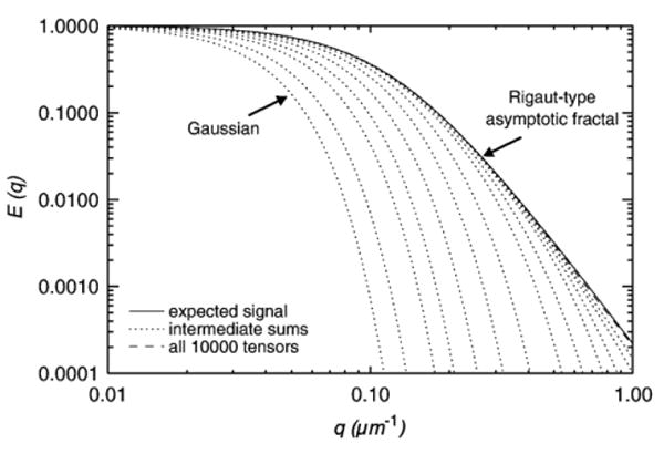
The Wishart distributed tensors lead to a Rigaut-type signal decay.

It is well known that the gamma distribution γ_p,σ with integer p is also the distribution of the sum of p independent random variables following exponential distribution with parameter σ. It follows from the central limit theorem that if p (not necessarily an integer) is large, the gamma distribution γ_p,σ can be approximated by the normal distribution with mean pσ and variance pσ². More precisely, the gamma distribution converges to a normal distribution when p goes to infinity. A similar behavior is exhibited by the Wishart distribution. Note that when p tends to infinity, we have

$$S(\text{q})\to S_0\text{exp}\left(-b{\text{g}}^T\widehat{\text{D}}\text{g}\right).$$ (12)

which implies that the mono-exponential model can be viewed as a limiting case (p→∞) of our model. Hence Eq. (10) can be seen as a generalization of Eq. (1). By the linearity of the Laplace transform, the bi-exponential and multi-exponential models can be derived from the Laplace transform of the discrete mixture of Wishart distributions as well.

Applications

A new framework for diffusion tensor estimation

The model in Eq. (5) also suggests a new method for the estimation of diffusion tensors from diffusion-weighted images. We first consider a set of diffusion measurements performed at a voxel containing a single fiber bundle. In this case, it is natural to use the Wishart distribution γ_p,Σ as the mixing distribution in Eq. (5) and thus the following equation is obtained:

$${\left(\frac{S_0}{S(\text{q})}\right)}^{1/p}-\text{trace}(\text{B}\sum )=1$$

or in the matrix form:

$$\left(\begin{array}{cccc}{(S_1)}^{-\frac{1}{p}}& B_{\text{xx}}& \dots & 2B_{\text{xz}}\\ {\left(S_2\right)}^{-\frac{1}{p}}& B_{\text{xx}}& \dots & 2B_{\text{xz}}\\ \dots & \dots & \dots & \dots \\ {(S_K)}^{-\frac{1}{p}}& B_{\text{xx}}& \dots & 2B_{\text{xz}}\end{array}\right)\left(\begin{array}{c}{(S_0)}^{\frac{1}{p}}\\ {\sum }_{\text{xx}}\\ \dots \\ {\sum }_{\text{xz}}\end{array}\right)=\left(\begin{array}{c}1\\ 1\\ \dots \\ 1\end{array}\right),$$ (13)

where K is the number of measurements at each voxel and B_ij and Σ_ij are the six components of the matrices B and Σ, respectively. Note that in the above expression the components of the matrices B and Σ should be ordered consistently. The final estimation of diffusion tensor Dˆ is obtained by taking the expected value of the Wishart distribution γ_p,Σ, i.e. Dˆ = pΣ.

Hence, the diffusion tensor estimation problem can be reformulated as the solution to a linear system. As a result, the S₀ and the six components in Σ can be estimated efficiently by using linear regression as has been customarily done in the traditional diffusion tensor estimation methods. Note that, since the focus of this paper is not simply the estimation of diffusion tensors from the DW-MRI measurements, as an application example of the proposed model, we chose to demonstrate that one may use a linear regression based formulation (as in the traditional DTI estimation) for estimating the diffusion tensors using the proposed Wishart mixing density model. Alternatively, one may use a nonlinear regression formulation for estimating the diffusion tensors and this would involve solving the following equation for pΣ using a non-linear least-squares technique such as the Levenberg–Marquardt algorithm (Press et al., 1992):

$$\underset{\sum }{min}{\left(S(\text{q})-S_0{(1+\text{trace}(\text{B}\sum ))}^{-p}\right)}^2$$ (14)

Note that in this nonlinear least-squares formulation, the data does not undergo any transformation prior to estimation of the diffusion tensors. In the results reported in the first subsection of Experiments, we use this nonlinear least-squares formulation to estimate the diffusion tensors and compare the accuracy of estimation to that obtained from a nonlinear least-squares estimation of pΣ but using the traditional mono-exponential Stejskal–Tanner model (Wang et al., 2004). In both the cases, the solution obtained from the corresponding linear-regression formulations are used as the initialization for the Levenberg–Marquardt nonlinear solver. For reasonably high signal-to-noise ratio, the solutions from the linear regression and the nonlinear least-squares are very close as was observed for the Stejskal–Tanner model in Basser et al. (1994).

It should be pointed out that many complicated methods which involve nonlinear optimization and enforce the positivity constraint on the diffusion tensor, as in (Chefd'hotel et al., 2004; Wang et al., 2004), can be applied to the Wishart model proposed here. Similarly, the resulting diffusion tensor field represented by the estimated pΣ at each voxel and can be then analyzed by numerous existing diffusion tensor image analysis methods (Weickert and Hagen, 2005).

Multi-fiber reconstruction using deconvolution

However, the single Wishart model can not resolve the intra-voxel orientational heterogeneity due to the single diffusion maximum in the model. Actually, the Laplace transform relation between the MR signal and the probability distributions on _n naturally leads to an inverse problem: to recover a distribution on _n that best explains the observed diffusion signal. In order to make the problem tractable, several simplifying assumptions are made as follows.

We first propose a discrete mixture of Wishart distribution model where the mixing distribution in Eq. (5) is expressed as $\text{d}F={\sum }_{i=1}^N{w}_i{\text{d}\gamma }_{p_i,{\sum }_i}$. In this model (p_i,Σ_i) are treated as basis and will be fixed as described below. This leaves us with the weights w, as the unknowns to be estimated. Note the number of components in mixture, N, only depends on the resolution of the manifold discretization and should not be interpreted as the expected number of fiber bundles. We assume that all the p_i take the same value p = 2 based on the analogy between the Eq. (10) and Debye–Porod law of diffraction (Sen et al., 1995) in three-dimensional space as discussed in the section of Theory. Since the fibers have an approximately cylindrical geometry, it is reasonable to assume that the two smaller eigenvalues of diffusion tensors are equal. In practice, we fix the eigenvalues of D_i = pΣ_i to specified values (λ₁, λ₂, λ₃) = (1.5, 0.4, 0.4)μ²/ms consistent with the values commonly observed in the white-matter tracts (Tuch et al., 2002). This rotational symmetry leads to a tessellation where N unit vectors evenly distributed on the unit sphere are chosen as the principal directions of Σ_i. In this way, the distribution can be estimated using a spherical deconvolution scheme (Tournier et al., 2004). For K measurements with q_j, the signal model equation:

$$S(\text{q})=S_0\sum _{i=1}^N{w}_i{(1+\text{trace}(\text{B}{\sum }_i))}^{-p}$$ (15)

leads to a linear system Aw = s, where s = (S(q)/S₀) is the vector of normalized measurements, w = (w_i), is the vector of weights to be estimated and A is the matrix with A_ji = (1 + trace(B_jΣ_i))^−p. It is worth noting that if we take p = ∝, the deconvolution kernel becomes the Gaussian function and the resulting w resembles very closely the fiber orientation estimated using continuous axially symmetric tensors (FORECAST) method proposed in Anderson (2005).

To avoid an under-determined system, K ≥ N is required without an interpolation on the measurements or exploring the sparsity constraints on w. Since the matrix A only depends on the sampling scheme and therefore needs only one-time computation, the computational burden of this method is light and comparable to that of the traditional linear least squares estimation of diffusion tensors from the Stejskal–Tanner equation. However, the induced inverse problem can be ill-conditioned due to the possible singular configurations of the linear system. In practice, we employ the damped least squares (DLS) (Wampler, 1986) inverse to overcome the instability problem. Instead of inverting small singular values, the damped least squares technique builds a smooth function converging to zero when the singular value tends towards zero. Note that the DLS is the closed form solution to one special case of the Tikhonov regularization used in Tournier et al. (2006).

Özarslan et al. (2006b) have shown that the distinct fiber orientations can be estimated by computing the peaks of the probability profiles, i.e. the probabilities for water molecules to move a fixed distance along different directions. Using a similar idea, we now present a way to compute the displacement probabilities using the proposed continuous distribution of tensors model.

First, the displacement probabilities can be approximated by the Fourier transform P(r) = ∫E(q)exp(−iq · r)dq where E(q) = S(q)/S₀ is the MR signal attenuation. Assuming a continuous diffusion tensor model as in Eq. (4) with mixing distribution $F(\text{D})={\sum }_{i=1}^N{w}_i{\text{d}\gamma }_{p_i,{\sum }_i}$, we have

$$\begin{array}{l}P(\text{r})={\int }_{R^3}{\int }_{{\mathcal{P}}_n}\text{exp}\left(-{\text{q}}^T\text{D}\text{q}t\right)\text{d}F(\text{D})\text{exp}(-i\text{q}\cdot \text{r})\text{d}\text{q}\\ \approx \sum _{i=1}^N\frac{w_i}{\sqrt{{(4\pi t)}^3|{\widehat{\text{D}}}_i|}}\text{exp}\left(-{\text{r}}^T{\widehat{\text{D}}}_i^{-1}\text{r}/4t\right)\end{array}$$ (16)

where Dˆ_i = pΣ_i are the expected values of γ_p,Σ_i.

After the displacement probability profile is computed as a real-valued function on the sphere, we represent all the resulting probability profiles in terms of spherical harmonics series and only the spherical harmonics expansion coefficients are stored for later visualization and finding fiber orientations. The existence of analytical angular derivatives of spherical harmonic functions enables the use of fast numerical optimization routines to find the peaks of the probability surfaces. However, due to the noise and truncation artifacts introduced in the finite order spherical harmonics expansion, we use a numerical optimization in conjunction with a heuristic approach in order to estimate the distinct fiber orientations. We first select a large number of randomly sampled points on the sphere and evaluate the spherical harmonic expansion of the probability profile at each of these points, and find the local maxima by searching within a fixed radius neighborhood. Then, a Quasi-Newton method was used to refine the position of each local maximum. Finally, we remove duplicate local maxima and any insignificant spikes with function values smaller than some threshold. The result of this heuristic pruning leads to significant maxima that correspond to the fiber orientations.

Experiments

A series of experiments were performed on synthetic data sets and on real rat brain data sets in order to evaluate the behavior of the proposed continuous tensor distribution model, as well as to validate the methods developed for diffusion tensor estimation and multi-fiber reconstruction, respectively.

Diffusion tensor field estimation using Wishart model

The first experiment was designed to assess the method proposed in the first subsection of Applications on a synthetic data set. The simulations employed the exact form of the MR signal attenuation from particles diffusing inside cylindrical boundaries (Söderman and Jönsson, 1995). The data set used in this experiment was generated to represent single-fiber diffusion with sinusoidally varying orientations as shown in Fig. 2(a).

Fig. 2.

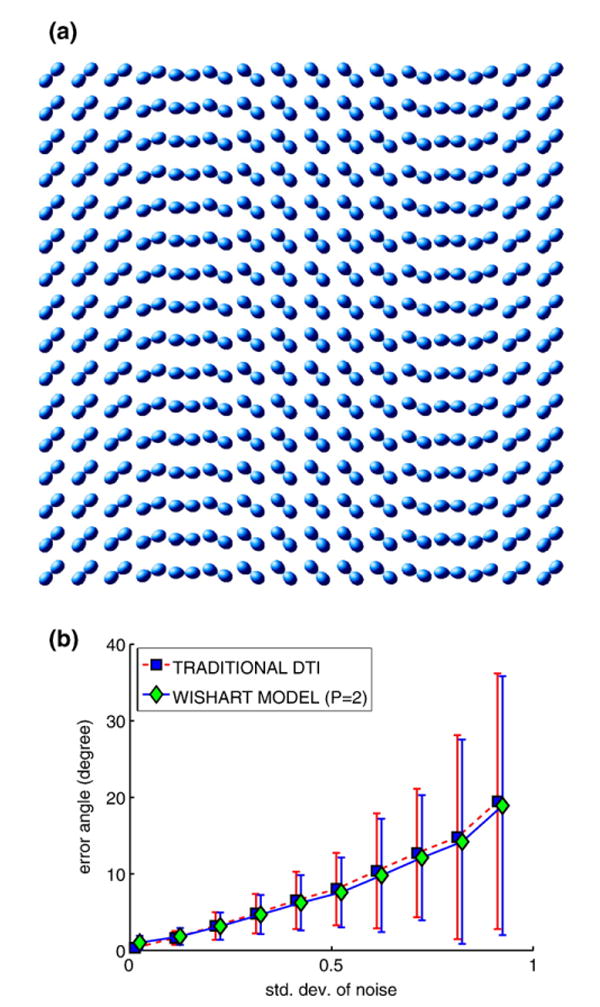
Diffusion tensor fitting of a simulated data set. (a) Visualization of the noiseless tensor field. (b) Comparison of the accuracy of the estimated dominant eigenvectors using different methods under different noise levels.

To quantitatively compare the accuracy of the tensor fits obtained using the proposed Wishart model and the traditional mono-exponential Stejskal–Tanner equation, we added different levels of Rician-distributed noise to the synthetic data set and then computed the angular deviation (in degrees) between the dominant eigenvector of the estimated diffusion tensor field and the ground truth orientation field which was used to generate the synthetic data set. Rician noise was imposed on the magnitude MR signal by using additive independent Gaussian noise on the real and imaginary parts of the complex-valued MR signal and taking its magnitude. For more details on this technique of approximating Rician noise, we refer the reader to Gudbjartsson and Patz (1995).

Fig. 2(b) shows the statistics of deviation angles obtained by applying the two different models (ours and the traditional Stejskal–Tanner model) to the synthetic data with increasing levels of Rician-distributed noise (σ = .01, …, .09) imposed on the magnitude of the MR signal. From the figure, we can see that the overall accuracy of these two models are very close to each other. However, the average angle errors using the Wishart model are lower than those obtained using the mono-exponential Stejskal–Tanner equation for increasing levels of noise.

Multi-fiber reconstruction on simulated data

We have applied the scheme described in the second subsection of Applications to the simulations of single fiber and crossing fiber systems. As in previous experiments, the simulations were performed following the exact form of the MR signal attenuation from particles diffusing inside cylindrical boundaries (Söderman and Jönsson, 1995).

Fig. 3 shows the probability surfaces for a simulated image of two-fiber crossing bundles computed using the proposed method. The surfaces are consistent with the underlying known fibrous structure. The curved and linear fiber bundles were chosen so that a distribution of crossing angles is achieved across the region with orientational heterogeneity. We notice that distinct fiber orientations are better resolved when the different fiber bundles make larger angles with each other.

Fig. 3.

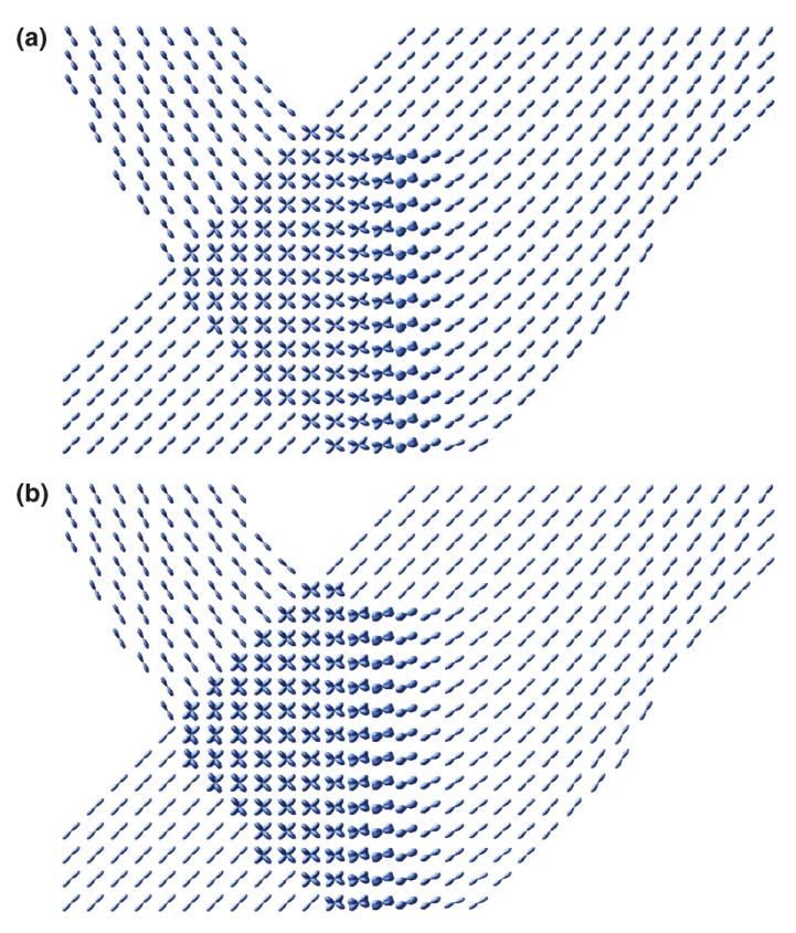
Probability maps from a simulated image of two crossing fiber bundles computed using (a) DOT and (b) proposed method.

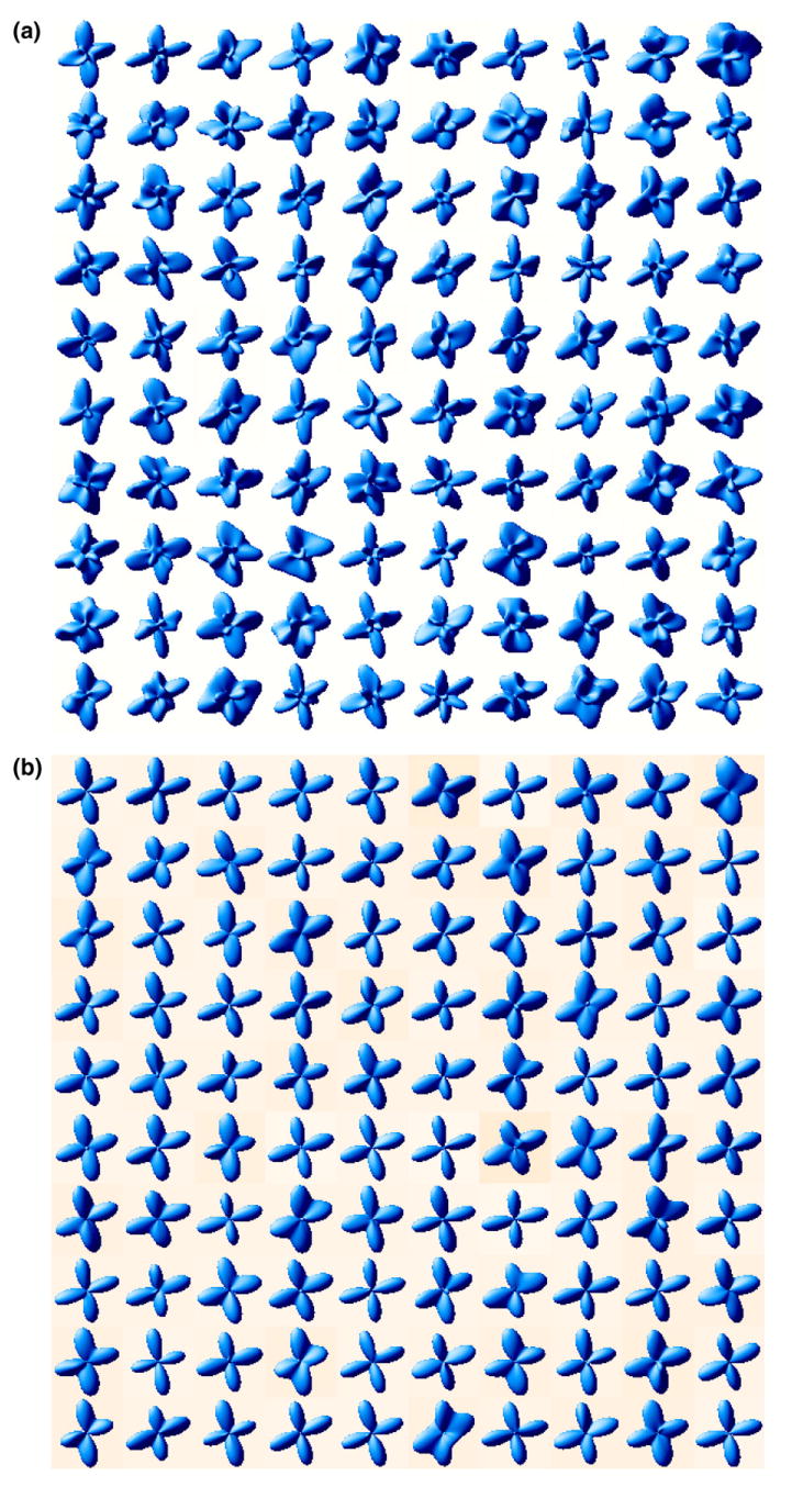
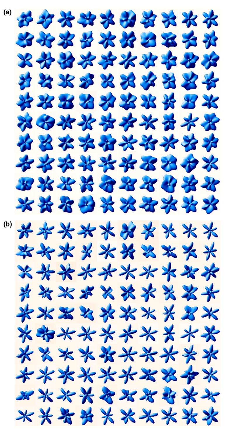
We also empirically investigated the performance of our reconstruction method. Of special interest is its accuracy in fiber orientation detection in the presence of noise. To study this problem, we first took the HARDI simulations of 1-, 2- and 3-fiber crossing profiles with known fiber orientations and computed the probability profiles which are depicted in Fig. 4.

Fig. 4.

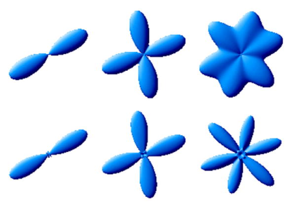
Simulations of 1, 2 and 3 fibers (b = 1500 s/mm²). Orientations: azimuthal angles φ₁ = 30, φ₂ = {20, 100}, φ₃ = {20, 75, 135}; polar angles were all 90°. Top: Q-ball ODF surfaces; Bottom: Probability surfaces computed using proposed method.

In the case of the noiseless signal, the proposed method as well as QBI and DOT are all able to recover the fiber orientation quite accurately. The Q-ball orientation distribution functions (ODF) is computed by using the spherical harmonic expansion formula given in Anderson (2005, Eq. (21)). Since our method and the non-parametric DOT method compute the probability values directly, we fit the resulting probability profiles from proposed method and DOT using spherical harmonics basis for the purpose of better surface display via rendering. The existence of analytical angular derivatives of spherical harmonic functions also enables us to apply fast gradient-based numerical optimization routines (described earlier) to find the peaks of the probability surfaces.

To provide a more quantitative assessment of the proposed method and its sensitivity to noise, we performed a series of experiments as follows:

• For all the 1-, 2- and 3-fiber crossing systems as shown in Fig. 4, the noise profile was created as described in the first subsection of Experiments with increasing noise levels (σ = .02, .04, .06, .08).

• For each noise corrupted fiber system, we recomputed the probability profiles by using the proposed method and DOT. Similarly, the Q-ball ODF were computed using the formula given by Anderson (2005, Eq. (21)). All the resulting surfaces were represented by spherical harmonics coefficients.

• We then estimated the fiber orientations of each system by numerically finding the maxima of the probability surfaces with a Quasi-Newton numerical optimization algorithm and computed the deviation angles ψ between the estimated and the true fiber orientations. In this case, since the ground truth fiber orientations were known, the initial orientations were chosen from random perturbations about the known ground truth fiber orientations.

• For each system and each noise level, the above steps were repeated 100 times to provide a distribution of deviation angles. Table 1 reports the mean and standard deviation of these distributions in degrees.

Table 1.

Mean and standard deviation values for the deviation angles ψ between the computed and true fiber orientations after adding Rician noise of increasing noise levels σ

	ψ (σ = 0)	ψ (σ = 0.02)	ψ (σ = 0.04)	ψ (σ = 0.06)	ψ (σ = 0.08)
From proposed method
1 fiber	{0.243}	0.65±0.39	1.19±0.65	1.66±0.87	2.19±1.27
2 fibers	{0.74}	1.18±0.66	2.55±1.29	3.85±2.12	4.91±3.26
	{0.69}	1.30±0.66	2.76±1.34	3.63±1.91	5.11±2.65
3 fibers	{1.02}	4.87±3.23	8.59±5.82	11.79±6.86	13.84±8.73
	{0.97}	5.81±3.61	7.70±5.02	11.27±6.36	12.54±7.48
	{1.72}	4.92±3.32	7.94±4.59	12.57±7.09	14.27±7.66
From DOT
1 fiber	{0.414}	0.71±0.35	1.08±0.58	1.84±0.88	2.20±1.28
2 fibers	{1.55}	1.97±0.96	3.37±1.90	5.39±2.99	7.00±4.25
	{1.10}	1.73±1.00	3.28±1.87	4.78±2.37	6.29±3.19
3 fibers	{4.11}	7.89±5.71	10.82±6.66	14.56±8.74	16.68± 10.21
	{3.46}	6.94±3.70	11.28±5.98	16.92± 10.36	17.02± 10.95
	{1.68}	6.76±5.21	10.90±5.63	14.08±9.05	13.99±9.74
From QBI
1 fiber	{0.089}	1.28±0.75	3.34±1.97	5.94±3.19	7.67±4.16
2 fibers	{0.45}	2.39±1.26	4.82±2.44	7.95±4.45	8.91±4.64
	{0.42}	2.30±1.10	4.94±2.15	7.49±3.88	9.34±4.45
3 fibers	{0.90}	10.80±5.59	12.15±4.42	20.21± 11.10	18.78± 11.39
	{0.90}	11.59±5.44	13.07±4.74	19.54± 11.80	20.79± 10.81
	{0.19}	11.66±5.18	12.25±4.93	20.36±11.50	19.10± 10.18

Note, in all cases, we discarded very large deviation angles that are greater than 30° when σ = 0.02, 40° when σ = 0.04, 50° when σ = 0.06 or σ = 0.08 since these large errors are mostly due to the failure of the numerical optimization routine.

As expected, the deviation angles between the recovered and the true fiber orientations increase with increasing noise levels and it is more challenging to accurately resolve the distinct orientations when there are more fiber orientations. The statistics reported in Table 1 also indicate that the proposed method has stronger resistance to the noise than the DOT and the QBI methods respectively. Figs. 5 and 6 also illustrate this finding.

Fig. 5.

Resistance to noise (2 fibers, σ = 0.08): (a) ODF from QBI; (b) Proposed method.

Fig. 6.

Resistance to noise (3 fibers, σ = 0.04): (a) ODF from QBI; (b) Proposed method.

Multi-fiber reconstruction on real data

The rat optic chiasm is an excellent experimental validation of our approach due to its distinct myelinated structure with both parallel and descussating optic nerve fibers. HARDI data from optic chiasm region of excised, perfusion-fixed rat nervous tissue was acquired at 14.1 T using Bruker Avance imaging systems. A diffusion-weighted spin echo pulse sequence was used. Diffusion-weighted images were acquired along 46 directions with a b-value of 1250 s/mm² along with a single image acquired at b ≈ 0 s/mm². Echo time and repetition time were 23 ms and 0.5 s respectively; Δ value and δ value were 12.4 ms and 1.2 ms; bandwidth was set to 35 kHz; signal average was 10; matrix size was 128 × 128 × 5 and resolution was 33.6 × 33.6 × 200 μm³. The optic chiasm images were signal-averaged to 67.2 × 67.2 × 200 μm³ resolution prior to probability calculations.

Fig. 7 shows the displacement probabilities computed from the optic chiasm image. For the sake of clarity, we excluded every other pixel and overlaid the probability surfaces on generalized anisotropy (GA) maps (Özarslan et al., 2005). As evident from this figure, our method is able to demonstrate the distinct fiber orientations in the central region of the optic chiasm where ipsilateral myelinated axons from the two optic nerves cross and form the contralateral optic tracts.

Fig. 7.

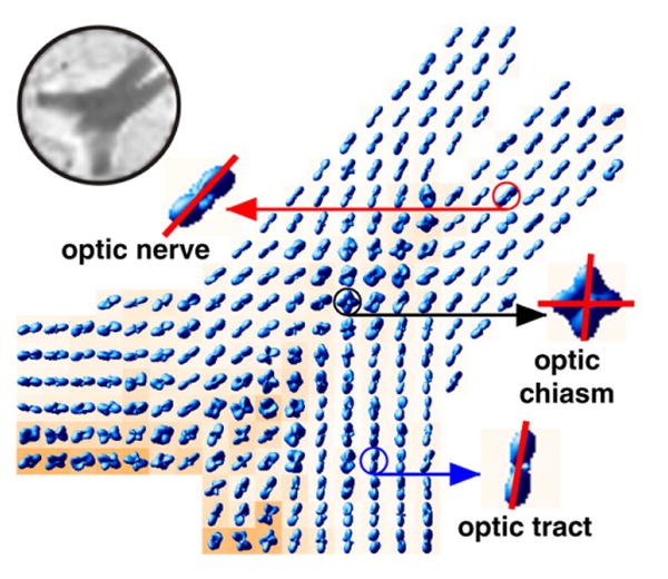
Probability maps computed from a rat optic chiasm data set overlaid on axially oriented GA maps. The decussations of myelinated axons from the two optic nerves at the center of the optic chiasm are readily apparent. Decussating fibers carry information from the temporal visual fields to the geniculate body. Upper left corner shows the corresponding reference (S₀) image.

To investigate the capability of diffusion-weighted imaging in revealing the effects in local tissue caused by diseases or neurologic disorders, further experiments were carried out on two data sets collected from a pair of epileptic/normal rat brains.

Under deep anesthesia, a Sprague-Dawley rat was transcardially exsanguinated and then perfused with a fixative solution of 4% paraformaldehyde in phosphate-buffered saline (PBS). The corpse was stored in a refrigerator overnight then the brain was extracted and stored in the fixative solution. For MR measurements, the brain was removed from the fixative solution then soaked in PBS, without fixative, for approximately 12 h (overnight). Prior to MR imaging, the brain was removed from the saline solution and placed in a 20-mm tube with fluorinated oil (Fluorinert FC-43, 3M Corp., St. Paul, MN) and held in place with plugs. Extra care was taken to remove any air bubbles in the sample preparation.

The multiple-slice diffusion-weighted image data were measured at 750 MHz using a 17.6 T, 89 mm bore magnet with Bruker Avance console (Bruker NMR Instruments, Billerica, MA). A spin-echo, pulsed-field-gradient sequence was used for data acquisition with a repetition time of 1400 ms and an echo time of 28 ms. The diffusion-weighted gradient pulses were 1.5 ms long and separated by 17.5 ms. A total of 32 slices, with a thickness of 0.3 mm, were measured with an orientation parallel to the long-axis of the brain (slices progressed in the dorsal–ventral direction). These slices have a field-of-view 30 mm × 15 mm in a matrix of 200 × 100. The diffusion-weighted images were interpolated to a matrix of 400 × 200 for each slice. Each image was measured with 2 diffusion weightings: 100 and 1250 s/mm². Diffusion-weighted images with 100 s/mm² were measured in 6 gradient directions determined by the vertices of an icosahedron in one of the hemispheres. The images with a diffusion-weighting of 1250 s/mm² were measured in 46 gradient directions, which are determined by the tessellations of the icosahedron on the same hemisphere. The 100 s/mm² images were acquired with 20 signal averages and the 1250 s/mm² images were acquired with 5 signal averages in a total measurement time of approximately 14 h.

Fig. 8 shows the displacement probabilities calculated from excised coronal rat brain MRI data in (a) a control and (b) an epileptic rat. The hippocampus and entorhinal cortex is expanded and it depicts the orientations of the highly anisotropic and coherent fibers. Note voxels with crossing orientations located in the dentate gyrus (dg) and entorhinal cortex (ec). The region superior to CA1 represent the stratum lacunosum–moleculare and statum radiatum. Note that in the control hippocampus, the molecular layer and stratum radiatum fiber orientations paralleled the apical dendrites of granule cells and pyramidal neurons, respectively. In the epileptic hippocampus, the CA1 subfield pyramidal cell layer is notably lost relative to the control. The architecture of the dentate gyrus is also notably altered with more evidence of crossing fibers. Future investigations employing this method should improve our understanding of normal and pathologically altered neuroanatomy in regions of complex fiber architecture such as the hippocampus and entorhinal cortex.

Fig. 8.

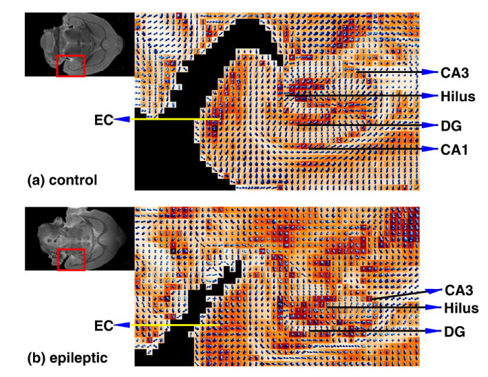
Probability maps of coronally oriented GA images of a control and an epileptic hippocampus. Upper left corner shows the corresponding reference (S₀) images where the rectangle regions enclose the hippocampi. In the control hippocampus, the molecular layer and stratum radiatum fiber orientations paralleled the apical dendrites of granule cells and pyramidal neurons respectively, whereas in the stratum lacunosum, moleculare orientations paralleled Schaffer collaterals from CA1 neurons. In the epileptic hippocampus, the overall architecture is notably altered; the CA1 subfield is lost, while an increase in crossing fibers can be seen in the hilus and dentate gyrus (dg). Increased crossing fibers can also be seen in the entorhinal cortex (ec). Fiber density within the statum lacunosum moleculare and statum radiale is also notably reduced, although fiber orientation remains unaltered.

Conclusion

In this paper, we presented a new mathematical model for the diffusion-weighted MR signals obtained from a single voxel. According to our model, the signal is generated by a continuous distribution of diffusion tensors, where the relevant distribution is a Wishart distribution. In this case, the MR signal was shown to be a Laplace transform of this distribution defined on the manifold of symmetric positive-definite tensors. We presented an explicit form of the expected MR signal attenuation given by a Rigaut-type asymptotic fractal formula. This form of the signal attenuation has the correct asymptotic dependence of the signal values on the diffusion gradient strength. Moreover, the angular dependence of the expected MR signal is different from the angular dependence implied by traditional DTI. The simulations of diffusion inside cylindrical boundaries suggested that the principal eigenvectors of the diffusion tensors obtained from the proposed model are more accurate than those implied by traditional DTI. Using this new model in conjunction with a deconvolution approach, we presented an efficient estimation scheme for the distinct fiber orientations and the water molecule displacement probability functions at each voxel in a HARDI data set. Both synthetic and real data sets were used to depict the performance of the proposed algorithms. Comparisons with competing methods from literature depicted our model in a favorable light.

Appendix A

A.1. Laplace transform on _n

For definition of Laplace transforms on _n, we follow the notations in Terras (1985).

Definition 3

The Laplace transform of f : _n→ , denoted by f, at the symmetric matrix Z∈ ^n×n is defined by Herz (1955):

$$\begin{array}{ll}\mathcal{L}f(\text{Z})={\int }_{{\mathcal{P}}_n}f(\text{Y})\text{exp}[-\text{trace}(\text{YZ})]\text{dY},& \text{where}\\ \text{dY}=\prod \text{d}{y}_{ij}1\le i\le j\le n.\end{array}$$ (17)

For a sufficiently nice function f, the integral above converges in the right half plane, Re(Z)>X₀ (Re(Z) denotes the real part of Z), meaning that Re(Z) − X₀∈ _n and the inversion formula for this Laplace transform is:

$$\begin{array}{c}\begin{array}{c}{(2\pi i)}^{-n(n+1)/2}{\int }_{\mathrm{Re}\text{Z}={\text{X}}_0}\mathcal{L}f(Z)\text{exp}[\text{trace}(\mathrm{YZ})]\\ \text{dZ}=\{\begin{array}{cc}f(\text{Y}),& \text{for}\text{Y}\in {\mathcal{P}}_{n,}\\ 0,& \text{otherwise}\text{.}\end{array}\end{array}\end{array}$$ (18)

Here dZ = Πdz_ij and the integral is over symmetric matrices Z with fixed real part.

If f is the density function of some probability measure F on _n with respect to the dominating measure dY, i.e. dF(Y) = f(Y)dY, then Eq. (17) also defines the Laplace transform of the probability measure F on _n which is denoted by F.

References

- Alexander DC. Maximum entropy spherical deconvolution for diffusion MRI. In: Christensen GE, Sonka M, editors. IPMI Lecture Notes in Computer Science. Vol. 3565. Springer; 2005. pp. 76–87. [DOI] [PubMed] [Google Scholar]
- Alexander DC, Barker GJ, Arridge SR. Detection and modeling of non-Gaussian apparent diffusion coefficient profiles in human brain data. Magn Reson Med. 2002 August;48(2):331–340. doi: 10.1002/mrm.10209. [DOI] [PubMed] [Google Scholar]
- Anderson TW. An Introduction to Multivariate Statistical Analysis. John Wiley and Sons; 1958. [Google Scholar]
- Anderson AW. Measurement of fiber orientation distributions using high angular resolution diffusion imaging. Magn Reson Med. 2005;54(5):1194–1206. doi: 10.1002/mrm.20667. [DOI] [PubMed] [Google Scholar]
- Assaf Y, Freidlin RZ, Rohde GK, Basser PJ. New modeling and experimental framework to characterize hindered and restricted water diffusion in brain white matter. Magn Reson Med. 2004;52(5):965–978. doi: 10.1002/mrm.20274. [DOI] [PubMed] [Google Scholar]
- Basser PJ, Mattiello J, LeBihan D. Estimation of the effective self-diffusion tensor from the NMR spin echo. J Magn Reson B. 1994;103:247–254. doi: 10.1006/jmrb.1994.1037. [DOI] [PubMed] [Google Scholar]
- Basser PJ, Pajevic S, Peierpaoli C, D J, Aldroubi A. In vivo fiber tractography using DT-MRI data. Magn Reson Med. 2000 October;44(4):625–632. doi: 10.1002/1522-2594(200010)44:4<625::aid-mrm17>3.0.co;2-o. [DOI] [PubMed] [Google Scholar]
- Behrens T, Woolrich M, Jenkinson M, Johansen-Berg H, Nunes R, Clare S, Matthews P, Brady J, Smith S. Characterization and propagation of uncertainty in diffusion-weighted MR imaging. Magn Reson Med. 2003;50(2):1077–1088. doi: 10.1002/mrm.10609. [DOI] [PubMed] [Google Scholar]
- Behrens T, Johansen-Berg H, Jbabdi S, Rushworth M, Woolrich M. Probabilistic tractography with multiple fibre orientations: what can we gain? NeuroImage. 2007;34:144–155. doi: 10.1016/j.neuroimage.2006.09.018. [DOI] [PMC free article] [PubMed] [Google Scholar]
- Callaghan P. Principles of Nuclear Magnetic Resonance Microscopy. Clarendon Press; Oxford: 1991. [Google Scholar]
- Chefd'hotel C, Tschumperlé, Deriche R, Faugeras O. Regularizing flows for constrained matrix-valued images. J Math Imaging Vis. 2004;20(1–2):147–162. [Google Scholar]
- Cleveland GG, Chang DC, Hazlewood CF, Rorschach HE. Nuclear magnetic resonance measurement of skeletal muscle: anisotropy of the diffusion coefficient of the intracellular water. Biophys J. 1976;16(9):1043–1053. doi: 10.1016/S0006-3495(76)85754-2. [DOI] [PMC free article] [PubMed] [Google Scholar]
- Conturo TE, Lori NF, Cull TS, Akbudak E, Snyder AZ, Shimony JS, McKinstry RC, Burton H, Raichle ME. Tracking neuronal fiber pathways in the living human brain. Proc Natl Acad Sci. 1999;96:10422–10427. doi: 10.1073/pnas.96.18.10422. [DOI] [PMC free article] [PubMed] [Google Scholar]
- Descoteaux M, Angelino E, Fitzgibbons S, Deriche R. A fast and robust ODF estimation algorithm in q-ball imaging. International Symposium on Biomedical Imaging: From Nano to Macro; 2006. pp. 81–84. [Google Scholar]
- Frank L. Characterization of anisotropy in high angular resolution diffusion weighted MRI. Magn Reson Med. 2002;47(6):1083–1099. doi: 10.1002/mrm.10156. [DOI] [PubMed] [Google Scholar]
- Gudbjartsson H, Patz S. The Rician distribution of noisy MRI data. Magn Reson Med. 1995;34(6):910–914. doi: 10.1002/mrm.1910340618. [DOI] [PMC free article] [PubMed] [Google Scholar]
- Herz CS. Bessel functions of matrix argument. Ann Math. 1955;61(3):474–523. [Google Scholar]
- Hess CP, Mukherjee P, Han ET, Xu D, Vigneron DB. Q-ball reconstruction of multimodal fiber orientations using the spherical harmonic basis. Magn Reson Med. 2006;56(1):104–117. doi: 10.1002/mrm.20931. [DOI] [PubMed] [Google Scholar]
- Hosey T, William G, Ansorge R. Inference of multiple fiber orientations in high angular resolution diffusion imaging. Magn Reson Med. 2005;54:1480–1489. doi: 10.1002/mrm.20723. [DOI] [PubMed] [Google Scholar]
- Jansons KM, Alexander DC. Persistent angular structure: new insights from diffusion MRI data. Inverse Problems. 2003;19:1031–1046. doi: 10.1007/978-3-540-45087-0_56. [DOI] [PubMed] [Google Scholar]
- Jian B, Vemuri BC, Özarslan E, Carney P, Mareci T. A Continuous Mixture of Tensors Model for Diffusion-Weighted MR Signal Reconstruction. IEEE 2007 International Symposium on Biomedical Imaging (ISBI'07); 2007. [DOI] [PMC free article] [PubMed] [Google Scholar]
- Köpf M, Metzler R, Haferkamp O, Nonnenmacher TF. NMR studies of anomalous diffusion in biological tissues: experimental observation of Lévy stable processes. In: Losa GA, Merlini D, Nonnenmacher TF, Weibel ER, editors. Fractals in Biology and Medicine. Vol. 2. Birkhäuser; Basel: 1998. pp. 354–364. [Google Scholar]
- LeBihan D, Breton E, Lallemand D, Grenier P, Cabanis E, Laval-Jeantet M. MR imaging of intravoxel incoherent motions: application to diffusion and perfusion in neurologic disorders. Radiology. 1986;161:401–407. doi: 10.1148/radiology.161.2.3763909. [DOI] [PubMed] [Google Scholar]
- Letac G, Massam H. Quadratic and inverse regressions for Wishart distributions. Ann Stat. 1998;26(2):573–595. [Google Scholar]
- Mori S, Crain BJ, Chacko VP, van Zijl PCM. Three-dimensional tracking of axonal projections in the brain by magnetic resonance imaging. Ann Neurol. 1999;45:265–269. doi: 10.1002/1531-8249(199902)45:2<265::aid-ana21>3.0.co;2-3. [DOI] [PubMed] [Google Scholar]
- Moseley ME, Cohen Y, Kucharczyk J, Mintorovitch J, Asgari HS, Wendland MF, Tsuruda J, Norman D. Diffusion-weighted MR imaging of anisotropic water diffusion in cat central nervous system. Radiology. 1990a;176(2):439–445. doi: 10.1148/radiology.176.2.2367658. [DOI] [PubMed] [Google Scholar]
- Moseley ME, Cohen Y, Mintorovitch J, Chileuitt L, Shimizu H, Kucharczyk J, Wendland MF, Weinstein PR. Early detection of regional cerebral ischemia in cats: comparison of diffusion and T2-weighted MRI and spectroscopy. Magn Reson Med. 1990b;14:330–346. doi: 10.1002/mrm.1910140218. [DOI] [PubMed] [Google Scholar]
- Murihead RJ. Aspects of Multivariate Statistical Theory. John Wiley and Sons; 1982. [Google Scholar]
- Özarslan E, Mareci TH. Generalized diffusion tensor imaging and analytical relationships between diffusion tensor imaging and high angular resolution diffusion imaging. Magn Reson Med. 2003;50(5):955–965. doi: 10.1002/mrm.10596. [DOI] [PubMed] [Google Scholar]
- Özarslan E, Vemuri BC, Mareci T. Fiber orientation mapping using generalized diffusion tensor imaging. International Symposium on Biomedical Imaging: From Nano to Macro; 2004. pp. 1036–1038. [Google Scholar]
- Özarslan E, Vemuri BC, Mareci TH. Generalized scalar measures for diffusion MRI using trace, variance, and entropy. Magn Reson Med. 2005;53(4):866–876. doi: 10.1002/mrm.20411. [DOI] [PubMed] [Google Scholar]
- Özarslan E, Basser PJ, Shepherd TM, Thelwall PE, Vemuri BC, Blackband SJ. Observation of anomalous diffusion in excised tissue by characterizing the diffusion–time dependence of the MR signal. J Magn Reson. 2006a;183(2):315–323. doi: 10.1016/j.jmr.2006.08.009. [DOI] [PubMed] [Google Scholar]
- Özarslan E, Shepherd TM, Vemuri BC, Blackband SJ, Mareci TH. Resolution of complex tissue microarchitecture using the diffusion orientation transform (DOT) NeuroImage. 2006b;31:1086–1103. doi: 10.1016/j.neuroimage.2006.01.024. [DOI] [PubMed] [Google Scholar]
- Press W, Flannery B, Teukolsky S, Vetterling W. Numerical Recipes in C: The Art of Scientific Computing. Cambridge Univ. Press; 1992. [Google Scholar]
- Rigaut JP. An empirical formulation relating boundary lengths to resolution in specimens showing ‘non-ideally fractal’ dimensions. J Microsc. 1984;133:41–54. [Google Scholar]
- Sen PN, Hürlimann MD, de Swiet TM. Debye–Porod law of diffraction for diffusion in porous media. Phys Rev B. 1995;51(1):601–604. doi: 10.1103/physrevb.51.601. [DOI] [PubMed] [Google Scholar]
- Söderman O, Jönsson B. Restricted diffusion in cylindrical geometry. J Magn Reson B. 1995;117(1):94–97. [Google Scholar]
- Terras A. Harmonic Analysis on Symmetric Spaces and Applications. Springer; 1985. [Google Scholar]
- Tournier JD, Calamante F, Gadian DG, Connelly A. Direct estimation of the fiber orientation density function from diffusion-weighted MRI data using spherical deconvolution. NeuroImage. 2004;23(3):1176–1185. doi: 10.1016/j.neuroimage.2004.07.037. [DOI] [PubMed] [Google Scholar]
- Tournier JD, Calamente F, Connelly A. Improved characterisation of crossing fibres: spherical deconvolution combined with Tikhonov regularization. Proceedings of the ISMRM 14th Scientific Meeting and Exhibition; Seattle, Washington. 2006. [Google Scholar]
- Tuch DS. Q-ball imaging. Magn Reson Med. 2004;52(6):1358–1372. doi: 10.1002/mrm.20279. [DOI] [PubMed] [Google Scholar]
- Tuch DS, Weisskoff RM, Belliveau JW, Wedeen VJ. High angular resolution diffusion imaging of the human brain. Proc. of the 7th ISMRM; Philadelphia. 1999. p. 321. [Google Scholar]
- Tuch DS, Reese TG, Wiegell MR, Makris N, Belliveau JW, Wedeen VJ. High angular resolution diffusion imaging reveals intravoxel white matter fiber heterogeneity. Magn Reson Med. 2002;48(4):577–582. doi: 10.1002/mrm.10268. [DOI] [PubMed] [Google Scholar]
- Tuch DS, Reese TG, Wiegell MR, Wedeen VJ. Diffusion MRI of complex neural architecture. Neuron. 2003 December;40:885–895. doi: 10.1016/s0896-6273(03)00758-x. [DOI] [PubMed] [Google Scholar]
- von dem Hagen E, Henkelman R. Orientational diffusion reflects fiber structure within a voxel. Magn Reson Med. 2002;48(3):454–459. doi: 10.1002/mrm.10250. [DOI] [PubMed] [Google Scholar]
- Wampler CW. Manipulator inverse kinematic solution based on damped least-squares solutions. IEEE Trans Syst Man Cybern. 1986;16(1):93–101. [Google Scholar]
- Wang Z, Vemuri BC, Chen Y, Mareci TH. A constrained variational principle for direct estimation and smoothing of the diffusion tensor field from complex DWI. IEEE Trans Med Imag. 2004;23(8):930–939. doi: 10.1109/TMI.2004.831218. [DOI] [PubMed] [Google Scholar]
- Wedeen VJ, Reese T, Tuch DS, Weigl MR, Dou JG, Weiskoff R, Chesler D. Mapping fiber orientation spectra in cerebral white matter with Fourier transform diffusion MRI. Proc of the 8th ISMRM; Denver. 2000. p. 82. [Google Scholar]
- Weickert J, Hagen H, editors. Visualization and Processing of Tensor Fields. Springer; 2005. [Google Scholar]
- Wishart J. The generalized product moment distribution in samples from a normal multivariate population. Biometrika. 1928;20:32–52. [Google Scholar]
Associated Data
This section collects any data citations, data availability statements, or supplementary materials included in this article.