Abstract
Molecular dynamics (MD) simulations generate a canonical ensemble only when integration of the equations of motion is coupled to a thermostat. Three extended phase space thermostats, one version of Nosé–Hoover and two versions of Nosé–Poincaré, are compared with each other and with the Berendsen thermostat and Langevin stochastic dynamics. Implementation of extended phase space thermostats was first tested on a model Lennard-Jones fluid system; subsequently, they were implemented with our physics-based protein united-residue (UNRES) force field MD. The thermostats were also implemented and tested for the multiple-time-step reversible reference system propagator (RESPA). The velocity and temperature distributions were analyzed to confirm that the proper canonical distribution is generated by each simulation. The value of the artificial mass constant, Q, of the thermostat has a large influence on the distribution of the temperatures sampled during UNRES simulations (the velocity distributions were affected only slightly). The numerical stabilities of all three algorithms were compared with each other and with that of microcanonical MD. Both Nosé–Poincaré thermostats, which are symplectic, were not very stable for both the Lennard-Jones fluid and UNRES MD simulations started from nonequilibrated structures which implies major changes of the potential energy throughout a trajectory. Even though the Nosé–Hoover thermostat does not have a canonical symplectic structure, it is the most stable algorithm for UNRES MD simulations. For UNRES with RESPA, the “extended system inside-reference system propagator algorithm” of the RESPA implementation of the Nosé–Hoover thermostat was the only stable algorithm, and enabled us to increase the integration time step.
INTRODUCTION
Molecular Dynamics (MD) is a fundamental technique used to study various molecular systems, and is especially useful in the study of protein folding. MD generates a classical trajectory by integrating Newton’s equations of motion. The first use of MD may be tracked back to the 1950’s, when innovative work was done by Alder and Wainwright on the equilibrium properties of hard-sphere particles to obtain the equations of state and the Maxwell–Boltzman distribution of velocities.1, 2 Since then, MD has been used in condensed matter and biophysical simulations, and is especially important for protein folding studies.3 MD is useful because it provides information, not only about the equilibrium properties (thermodynamic averages), but also about the dynamical (kinetic) properties of the system studied (which includes the time dependence and fluctuation magnitude).
Conventional MD generates a microcanonical ensemble (NVE), in which the total number of particles, volume of the system, and energy are conserved. The benefit of this conservation of energy is that it allows one to test the numerical stability of the simulation. However, when comparing theoretical to experimental data, it is more common to use the canonical ensemble (NVT), in which temperature, instead of energy, is conserved. Several extensions of MD algorithms have been proposed to generate a canonical ensemble.
One of the earliest such algorithms, proposed by Anderson, applies stochastic collisions and randomly chooses the particle for resetting the velocity from the Maxwell–Boltzmann distribution for a given temperature.4 However, due to discontinuities in the trajectories, and because the algorithm does not provide a valid method to evaluate how the system is working (because there is no conserved quantity for which to test), Andersen’s method is not used widely. Employing the same principle used by Andersen, that of a stochastic thermostat, Langevin dynamics may be used to generate a canonical ensemble.
Langevin stochastic dynamics utilizes friction and random forces to keep temperature constant. The average magnitude of the random forces and the friction are related in such a way as to guarantee that the fluctuation-dissipation theorem is obeyed.5 Langevin stochastic dynamics closely reproduces the physical principles which are responsible for the generation of a canonical ensemble. Langevin dynamics is often used as a reference for other thermostat algorithms. The only disadvantage is that there is no conserved quantity with which to measure the accuracy of the Langevin stochastic dynamics used in the simulation.6 Berendsen et al. modified this Langevin equation to introduce only global coupling between the system studied and the heat bath.7 The global coupling is realized by supplementing the equation of motion by a first-order equation for the kinetic energy, in which the difference between the instantaneous kinetic energy and its target value is the driving force.7 Although Berendsen produced a very popular, stable algorithm, it is not associated with a well-defined ensemble8 (i.e., it does not generate the exact canonical ensemble), and it still lacks a conserved quantity; therefore, it is not an ideal algorithm.
In order to overcome the shortcomings of the Berendsen algorithm, Nosé introduced a method that generates the exact canonical distribution by extending the Hamiltonian.9, 10 This extended Hamiltonian (H) consists of the Hamiltonian of the physical system and an additional term describing the kinetic and potential energy associated with the degrees of freedom representing the thermostat. Conservation of this extended Hamiltonian may then be used to test the stability of the algorithm. The Nosé–Hoover thermostat10, 11 is obtained through noncanonical transformations of the variables from the equations of motion that do not leave the form of the Hamiltonian equations invariant.12 This is the reason why the symplectic algorithm (i.e., the algorithm whose numerical solution is exact for the perturbed Hamiltonian up to an exponentially small error13) cannot be employed directly with the Nosé–Hoover thermostat.
Bond et al.13 used Poincaré time transformations14 in order to construct a system of invariant Hamiltonian equations which generate a canonical ensemble. This facilitates implementation of the numerical integrator with the symplectic property.13 Following this work, Nosé designed an explicit symplectic integration algorithm for the Nosé–Poincaré thermostat.15
All-atom MD studies of protein folding are impractical because they do not allow a large enough time scale to be used for comparison with experimental data.3 By contrast, coarse-grained models, in which amino acids are represented by a few centers of interaction, extend the time scale of the simulation by several orders of magnitude. The time scale may be extended further by using a multiple-step reversible reference system propagator (RESPA).16, 17 In general, multiple-time-step methods work by dividing the forces into fast- and slow-varying ones; slow-varying forces are integrated with regular (large) time steps, while fast-varying forces are integrated with several, smaller substeps that are an integral fraction of the regular time step. The united-residue (UNRES) model is a physics-based coarse-grained one developed in our laboratory over the last several years, and has been extended for use with MD (Refs. 18, 19) and RESPA.20
In this work, we implemented the Nosé–Hoover and Nosé–Poincaré algorithms in UNRES molecular dynamics, both with and without RESPA, in an attempt to determine which is the better algorithm (in terms of both stability and computational time) for studying protein folding.
METHODS
The dynamics of a physical system consisting of particles with coordinates qi, momenta pi, masses mi, and interactions described by the potential V is expressed by Newton’s equations of motion,
| (1) |
These equations of motion can be integrated using the standard velocity Verlet algorithm.21, 22 The ensemble generated by solving these equations of motion is microcanonical (NVE), which conserves the total number of particles, volume of the system, and energy, and is the starting point for our work with thermostats that produce a canonical (NVT) ensemble, since NVE is not appropriate for comparing theoretical data with experimental data measured by NVT.
A key concern in MD simulations is the maintenance of constant temperature, either by using Langevin dynamics, in which friction and random forces compensate to maintain constant temperature, or by coupling the system to a thermostat. Our goal in implementing the Nosé–Hoover and Nosé–Poincaré algorithms was to determine which one was the most stable so that we could then integrate it with our UNRES model for MD simulations. Because Nosé–Hoover was considered to be a weaker algorithm, i.e., it is not a Hamiltonian system, even though it does have a conserved quantity [the total extended energy, Eext, defined in Eq. 3] that can be controlled and, although time reversible, it does not produce the desired canonical symplectic structure,13 we nevertheless decided to examine the performance of both Nosé–Hoover and Nosé–Poincaré methods with UNRES. In work by Bond et al.13 in 1999, the Nosé–Poincaré method was shown to be more stable than Nosé–Hoover; this algorithm was improved upon by Nosé in a paper from 2001.15 Here, we first implement the Nosé–Hoover (NH96) algorithm,12 and then the Nosé–Poincaré [NP01 (Ref. 15) and NP99 (Ref. 13)] algorithms, and compare them with the results of Berendsen and Langevin dynamics.
Both the Nosé–Hoover and Nosé–Poincaré thermostats are based on an extended Hamiltonian, which consists of a physical system of kinetic and potential energy, and also a term for the thermostat represented by a virtual particle. For our purposes, we introduced which describes the scaled momenta of the physical particles in the system with masses m; V represents the potential energy of the system as a function of its coordinates q. In the present context, V represents the Lennard-Jones potential energy or the UNRES potential energy. The position and momenta of the artificial particle representing the thermostat are denoted as s and π, respectively. A constant Q is the artificial mass of the thermostat particle. The number of degrees of freedom of the system is represented by g; k is the Boltzmann constant; and T is the temperature of the bath. It should be noted that the real momenta , and the kinetic energy of the system (Ek) is a function of the real momenta. Coupling between the thermostat and the physical system allows us to control and maintain the temperature constant.
Nosé–Hoover
The Nosé–Hoover algorithm was implemented because of its relevance to the other thermostats, even though it is not symplectic and not Hamiltonian but it is time reversible. The Nosé Hamiltonian is defined by
| (2) |
where η=ln s. The integration scheme used here is the one introduced by Martyna et al.12 (which is denoted here as NH96). In this scheme, the total extended energy (Eext), as opposed to the Hamiltonian (HNosé), is the conserved quantity, but Eext and HNosé are similar in form.
| (3) |
The equations of motion for the system may now be written as follows instead of Eq. 1:
| (4) |
and, for the thermostat particle,
| (5) |
The integration scheme for NH96 is described by the following equations, where the indices i indicate the real system particle number, the indices n and n+1 represent the discrete time step , and the other superscripts n+1∕2, *, and ** represent the intermediate variables between the nth and (n+1)th time steps.
| (6) |
| (7) |
| (8) |
| (9) |
| (10) |
| (11) |
| (12) |
| (13) |
| (14) |
| (15) |
| (16) |
| (17) |
In the NH96 scheme, there is a clear separation of the propagation of thermostat variables and the particle variables of the real system. Only the kinetic energy of the real system is used to update the thermostat variables at both the beginning and end of the scheme [Eqs. 6, 7, 8, 9, 13, 14, 15, 16, respectively]. Update of the real system variables uses , calculated during the thermostat updates, to scale the real momenta [Eqs. 10, 17].
The integration scheme proposed by Martyna et al.12 allows for multiple time steps and a higher-order algorithm to be applied for the thermostat part of the evolution operator (as seen in Eq. (29) of Martyna et al.12). We did not apply this feature in our studies so that the results could be compared to Nosé–Poincaré algorithms which do not have this feature.
Nosé–Poincaré
The Nosé–Poincaré Hamiltonian,13H, is derived from the original Nosé Hamiltonian HNosé by applying the Poincaré transformation of time.14
| (18) |
where differs from HNosé with g replacing g+1. The constant H0 is the value of under the initial conditions such that H will be initially zero. The equations of motion, using the Nosé–Poincaré Hamiltonian from Eq. 18, are as follows:
| (19) |
| (20) |
The following is the NP01 algorithm15 which couples the system and the thermostat defined by the Nosé–Poincaré algorithm:
| (21) |
| (22) |
| (23) |
| (24) |
| (25) |
| (26) |
| (27) |
| (28) |
Prior to this formulation of NP01 by Nosé,15 Bond et al.13 had used the integration scheme (denoted here as NP99) which we also implemented. The Hamiltonian used is H of Eq. 18. The following set of equations makes up the NP99 algorithm.13
| (29) |
| (30a) |
where C is the following constant from the solution of a quadratic equation [Eq. 35(b) of Ref. 13]:
| (30b) |
| (31) |
| (32) |
| (33) |
| (34) |
This integration scheme involves the solution of a quadratic term in Eqs. 30a, 30b. Therefore, unlike NP01, it is not fully explicit, but may be considered effectively explicit to distinguish it from methods which are implicit in the force terms. Also, the propagation of the momenta and coordinates of the real particles and those of the thermostat occurs in a different order in NP99 and in NP01. Nosé–Poincaré uses the virtual momenta instead of the real ones,pi, that are used by Nosé–Hoover. NP01 and NP99 have fewer steps than NH96. Also, unlike NH96, which uses four steps to update the thermostat velocity (π), NP01 and NP99 use only two steps.
Berendsen thermostat
Besides Nosé–Hoover and Nosé–Poincaré, the Berendsen algorithm and the Langevin algorithm were tested for comparison. In the Berendsen algorithm,7 the velocities at each step of the integration algorithm are scaled by a factor λ, as defined by Eq. 35.
| (35) |
Here, Δt is the integration time step, T0 is the bath temperature, T(t) is the instantaneous temperature as calculated from the kinetic energy, and τT is Berendsen’s coupling constant to the thermal bath. The selected τT is a compromise between a small value, which provides tight coupling to the thermostat, and hence a less natural trajectory (because of small fluctuations in kinetic energy and large fluctuations in the total energy), and a large value which provides a microcanonical rather than a canonical ensemble. In the Berendsen algorithm, coupling between the thermostat and the real system does not generate an exact canonical ensemble, and there is no conserved quantity with which to control the accuracy of the algorithm.
Langevin stochastic dynamics
The Langevin equation describes the stochastic dynamics of the system; in addition to the forces from the potential energy, friction and random forces are acting on each particle. The Langevin equation for a system of particles is described by Eq. 36.
| (36) |
where Ri(t) denotes the stochastic force acting on the generalized coordinate qi. Ri(t) is a δ-correlated function with zero mean, as expressed by Eqs. 36a, 36b.
| (36a) |
| (36b) |
As before, qi and mi are the coordinates and masses of the particles which interact with the potential V. Temperature is represented by T, and k is the Boltzmann constant. The friction coefficient is γ (obtained from Stokes law).
Model systems
Lennard-Jones fluid
In an initial test, the above algorithms were implemented with the model Lennard-Jones fluid system, which is the same model system used for the original development of all three thermostats. The system consisted of 108 particles in a cubic periodic box. The potential energy was calculated using a minimal image convention without cutoff distance as
| (37) |
The kinetic energy for the Lennard-Jones fluid was calculated using the equation
| (38) |
To compare with the results from Bond et al.,13 reduced units for ε, σ, and m, all equal to 1, were used. The system was simulated for half a million steps, under the following conditions: constant density ρ*=0.95 (reduced units, ρ*=ρσ3), constant temperature T*=6 (also in reduced units, T*=kTε−1), and Q=0.1. The initial configuration was generated by randomly placing the first particle in the box and then placing each sequential particle in the box in such a way as to prevent overlapping with the particles already inside. Initial velocities were generated from the Maxwell–Boltzmann distribution.
Values for the integration time step Δt* from 0.0001 to 0.01 were tested (with reduced units, t*=tσε1∕2m−1∕2). Specifically, the velocities and temperatures were calculated from the kinetic energy so that their distribution in comparison to the reference Boltzmann (Gaussian) distribution for a given temperature could be analyzed. Also, the conservation of the Hamiltonian and, in the case of Nosé–Hoover, the conservation of the total extended energy was of interest.
Polyglycine in UNRES
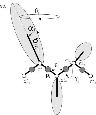
The primary goal of this work is the implementation of the most stable thermostat for coarse-grained UNRES MD simulations. In UNRES, each amino acid is represented by two centers of interaction: the united peptide group (p) located between two consecutive Cα atoms, and the united side chain3, 23 (SC) (Fig. 1). The UNRES effective energy is derived as a restricted free energy by integrating over the fine-grained degrees of freedom of the all-atom system and by using Kubo’s cumulant expansion.24
Figure 1.
The UNRES model for a polypeptide chain with the following centers of interaction: the united peptide group (pi) and the united side chain (SCi) represented by dark circles and ellipsoids, respectively. The open circles represent the Cα atoms which serve only as geometric points. The geometry of the chain is described by the virtual-bond angles θi, virtual-bond dihedral angles γi, and the angles αi and βi, and the bond lengths bsci that define the location of the side chain.
The UNRES energy function is described by the following equation:
| (39) |
Here USCiSCj, USCipj, and Upipj describe the inter-side-chain, the side chain–peptide, and the peptide-peptide interactions, respectively. The local terms, Utor, Utord, Ub, and Urot, correspond to the virtual-bond torsional, the double torsional, the virtual-bond angles θ, and the side-chain rotamers, respectively. Finally, are the correlation terms describing coupling between backbone-local and backbone-electrostatic interactions, while Ubond is the virtual-bond-stretching potential and USS is the disulfide-bond potential term accounting for breaking and forming of disulfide bonds.25 No truncation of the forces is used in UNRES simulations in contrast to the minimal image convention used in Lennard-Jones fluid simulations.
The internal parameters of Upipj, Utor, Utord, and were derived by fitting the analytical expressions to the restricted free energy surfaces of model systems computed at the quantum mechanical level.26, 27 The internal parameters of USCiSCj, USCipj, Ub, and Urot were derived28 by using distribution functions determined from the Protein Data Bank (PDB). The USCiSCj potential was refined by using a hierarchical optimization to derive the 4P force field.29 The Ubond has the form of a simple harmonic potential. The w’s are the weights associated with each energy term and are determined by hierarchical optimization.30 The most recent UNRES force field, optimized for canonical simulations, based on the 1GAB training protein with temperature dependence of the weights, was used.31 The energy-term weights are given in the last column of Table V of Ref. 31.
The Cartesian coordinates of the interacting sites in the UNRES model (which do not include Cα’s) are not sufficient to define the UNRES conformations. Therefore, the Lagrange formulation of the equations of motion has been adopted to describe the time evolution of a system characterized by a set of generalized coordinates. For the UNRES model, we chose the virtual-bond vectors and as the generalized coordinates q.19 The Cartesian coordinates x of the interacting sites and their velocities v are related to the generalized coordinates q and generalized velocities by Eqs. 40, 41, respectively.
| (40) |
| (41) |
where A is the transformation matrix from the generalized coordinates q to the Cartesian coordinates of the interacting sites x.19 The equation of motion for the UNRES model can be written as Eq. 42.
| (42) |
with the inertia matrix G defined by Eq. 43.
| (43) |
where U is the UNRES potential energy, M is the diagonal matrix of the masses of the interacting sites, and H is the part of the inertia matrix that corresponds to the internal (stretching) motions of the virtual bonds.19
The kinetic energy (Ek) for UNRES consists of two parts: one part arising from the UNRES degrees of freedom, and the second part arising from the average kinetic energy due to integration over the fine-grained degrees of freedom.19 The second part was assumed to be constant.19 Hence, the kinetic energy can be expressed by Eq. 44.
| (44) |
with
| (45) |
where the inertia matrix G is defined by Eq. 43, μi, i=1⋯n, are the eigenvalues of G, and V is the matrix of the eigenvectors of G.19 The velocities expressed in normal coordinates (ξ1,ξ2,…,ξn) have a normal distribution. The average distribution of velocities in the UNRES model is calculated from these normal coordinates computed from the generalized velocities using Eq. 45 and then scaled by as expressed by Eq. 46.
| (46) |
The projection and scaling of generalized velocities are necessary to analyze isothermal simulations in UNRES, as only the scaled quantities , i=1,2,…,n, should obey identical normal distributions with zero mean and variance equal to RT.
The UNRES energy is expressed in kcal∕mol, the mass of the system is in g∕mol, and the distance is in Å. The natural units of time for UNRES simulations is 48.9 fs, which is hereafter referred to as the molecular time unit (mtu).19 The effective UNRES unit of time is larger than 48.9 fs.32
As a model system for UNRES, a 20-residue polyglycine chain was used, and the system was simulated for two million steps at a bath temperature of 300 K. The stability was tested for time steps ranging from Δt=0.01 to Δt=0.30 with Q=0.5, and also with Q=1.0. The simulation was started from the extended polyglycine chain, and Maxwell–Boltzmann distributions were used to initialize the velocities for the target temperature.18 The implementation of the Berendsen and Langevin algorithms was described by Khalili et al.32
RESPA for the Nosé–Poincaré thermostat
For Nosé–Hoover, there already were two versions of multiple-time-step RESPA integration schemes designed by Martyna et al.,12 extended system outside-reference system propagator algorithm (XO-RESPA) and extended system inside-reference system propagator algorithm (XI-RESPA). However, because neither of the Nosé–Poincaré algorithms had been designed for RESPA, it was necessary to augment those algorithms here to fit RESPA.
RESPA versions of the Nosé–Poincaré algorithms NP99 and NP01 can be derived12, 16, 17, 33 following the general rules of Trotter factorization of the Liouville operator corresponding to the extended Hamiltonian given by Eq. 18, by splitting the Hamiltonian into two terms: fast-varying Hf, which allows only smaller time substeps, and slow-varying Hs, which allows large time steps, as expressed by Eqs. 47, 48, 49.
| (47) |
| (48) |
| (49) |
where Vs is the slow-varying potential energy, Vf is the fast-varying potential energy, and the total potential energy is V=Vs+Vf.20 The constant Csplit is chosen so that both Hf and Hs are zero at t=0. The time step for the small substep Δt′ is an integral fraction of the large time step, Δt′=Δt∕r, selected with RESPA split r. The equations of motion for Hs are as follows (without changing q or s in the integration of Hs):
| (50) |
| (51) |
The equations of motion for Hf are almost identical to those for the full Hamiltionian,
| (52) |
| (53) |
Applying the Nosé–Poincaré scheme to integrate the Hf Hamiltonian is the same as applying it to the full Hamiltonian except for the use of the fast-varying energy Vf, in place of the full potential energy V, and Csplit in place of H0.
The RESPA algorithm in both NP01 and NP99 versions has similar structure: in the first part of the large step, the velocities are propagated to half of the large time step using slow-varying forces; next, small substeps are iterated in a loop using fast-varying forces and the full NP01 or NP99 scheme with Vf, in place of the full potential energy V, and Csplit in place of H0; and, in the second part of the large step, the velocities are propagated from half of the large time step to the full large step using slow-varying forces.
RESPA was tried for all three of the aforementioned thermostats, each for several different numbers of substeps. A split (number of substeps) equal to 1 was used initially in order to compare the performance to that of the regular MD tests without RESPA, as they should correspond. Simulations were also run using splits equal to 2 and 4 (for both the Lennard-Jones system and polyglycine with UNRES), and 8 and 16 (for UNRES only). The split number was constant for a given run. For the Lennard-Jones fluid, we divided the forces acting on a given particle into slow- and fast-varying ones depending on the distance between the atom and the atom exerting force on it, as given by Eqs. (60) and (61) of Ref. 12; we used the same parameters of those equations as given in Ref. 12. For UNRES, the components were classified into slow- and fast-varying forces as in the work of Rakowski et al.20 Once again, the stability was tested for time steps ranging from Δt=0.01 to Δt=0.30 with Q=0.5. Each simulation ran for two million regular steps.
RESULTS AND DISCUSSION
Lennard-Jones fluid
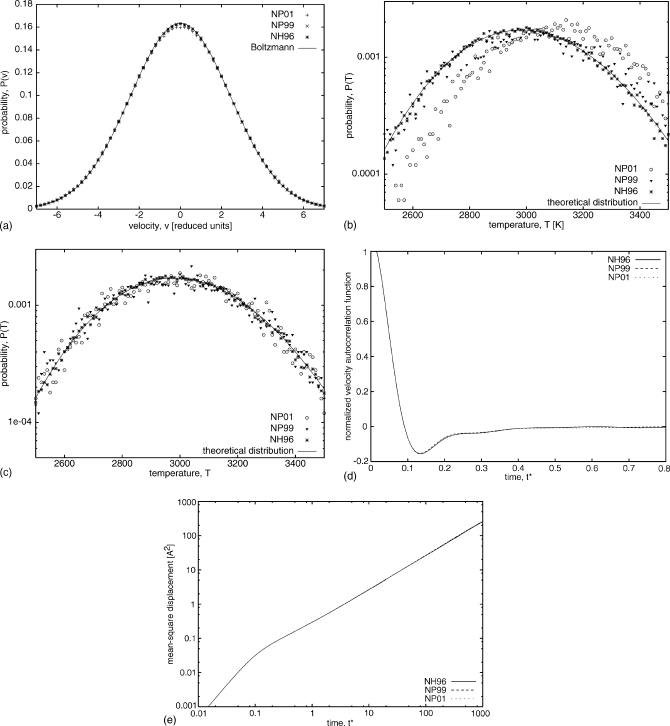
In order to test our implementation of the Nosé–Hoover (NH96) and Nosé–Poincaré (NP01 and NP99) thermostats, several MD simulations of a Lennard-Jones fluid were carried out. The distribution of the components of the velocity vectors was analyzed and compared with the Boltzmann (Gaussian) distribution for the given temperature (T*=6), as seen in Fig. 2a. The temperature distribution was also analyzed and compared to the theoretical distribution [Fig. 2b]. For all three thermostats, the distribution of velocities almost perfectly reproduced the theoretical distribution. For both Δt*=0.003 and Δt*=0.006, the differences between the simulated and theoretical distributions are very small, although the differences are slightly larger for Δt*=0.006 [Fig. 2a]. For the temperature distribution, however, only NH96 fits the theoretical distribution well; NP99 is close, but NP01 is shifted from the theoretical [Fig. 2b]. The results for temperature are closer to the theoretical distribution for Δt*=0.003 than for Δt*=0.006 [the distributions for Δt*=0.003 are represented in Fig. 2c]. The shift in kinetic energy distribution was studied by others and commonly is associated with insufficient ergodicity to provide the correct energetic distributions on the time scale of simulations or with a nonoptimal value for the thermostat mass Q,34, 35 but in these two simulations the only difference is the larger time step which should not affect the ergodicity.
Figure 2.
(a) Comparison of velocity distribution for Lennard-Jones fluid (108 particles, T*=6, ρ*=0.95, Δt*=0.006). Histograms were generated from simulations using thermostats: NP01 (pluses), NP99 (x’s), and NH96 (stars). The solid line is the theoretical Boltzmann (Gaussian) distribution: . (b) Comparison of temperature distribution for Δt*=0.006 [other same parameters as in (a)]. The theoretical distribution is of the form . The y axis is in a logarithmic scale. NP01 is represented by circles, NP99 by triangles, and NH96 by stars. (c) Comparison of temperature distribution for Δt*=0.003 [other parameters are the same as in (b)]. (d) Normalized velocity autocorrelation function for NP01 (dotted line), NP99 (dashed line), and NH96 (solid line). (e) The mean-square displacement as a function of time; both axes are in a logarithmic scale [line styles are the same as in (d)].
We have also investigated some dynamical quantities associated with time-correlated functions: the velocity autocorrelation functions [Fig. 2d] and mean-square displacements [Fig. 2e] as function of time for all three thermostats studied. In MD simulations, for this analysis we have used the same parameters as in Ref. 13 (T*=1.5, ρ*=0.95, Q=1.0, Δt*=0.005). Dynamics associated with all three algorithms, NH96, NP99, and NP01, evolve with the same time scale, and both the velocity autocorrelation function and mean-square displacement curves are almost identical for all three thermostats. The results are also close to the original data presented for the NP99 algorithm.13
To test the stability of the methods, the relative energy error (ΔE) was calculated with the formula
| (54) |
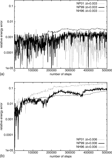
where E is Eext for Nosé–Hoover, and HNosé in the case of Nosé–Poincaré, at times zero and t, respectively. The results of these calculations may be seen in Fig. 3. For the small time step, Δt*=0.003, each method has a relatively stable and small ΔE (less than 0.005) whereas, for the larger time step, ΔE increases continuously, although still relatively small. For the small time step, NH96 had the largest ΔE, which is nearly twice as large as that of both NP01 and NP99. For the large time step, however, the situation is reversed; although the relative energy errors increase for each method, NH96 has the smallest values and NP01 the largest. The results with the NP99 method are similar to those of Bond et al.;13 the slightly larger ΔE’s appear here because no potential energy smoothing was imposed. Bond et al.13 used a truncated, shifted, and smoothed Lennard-Jones potential, while a simple truncated potential was used here. Numerical tests for the Lennard-Jones fluid illustrate that our implementations of the three thermostats are numerically stable.
Figure 3.
The relative energy errors, as a function of the number of steps, from the MD simulations of the Lennard-Jones fluid using step size (a) Δt*=0.003 and (b) Δt*=0.006 for two versions of Nosé–Poincaré (NP01, dotted line, and NP99, thick solid line) and Nosé–Hoover (NH96, thin solid line) thermostats. The relative energy error is in a logarithmic scale.
UNRES model of polyglycine
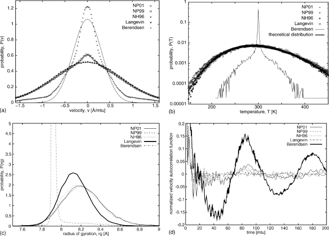
Turning to UNRES, the distributions of velocities from both Nosé–Poincaré and Nosé–Hoover algorithms were analyzed and compared with Langevin stochastic dynamics and the Berendsen thermostat [Fig. 4a]. The velocity distributions for NVE simulations were not analyzed because NVE was used only as a reference for the stability of our algorithms. It is clearly visible that the Berendsen thermostat produces a non-Gaussian distribution of velocity with a much higher maximum at zero velocity. Langevin provides an exact Boltzmann (Gaussian) distribution, and the other three thermostats introduced in this work for UNRES produced distributions of velocities close to Gaussian with only slightly higher maxima for zero velocity for Q=1.0. Detailed analysis of the distributions of all components of the scaled normal velocities shows that this slightly higher maximum is associated with the movement of the last virtual-bond vector which is not correlated enough with movement of the other virtual-bond vectors and with the thermostat. The problems with equipartition of kinetic energy have been reported for all-atom simulations in which the thermal distribution of light and heavy degrees of freedom converges very slowly to the average distribution.34 For smaller Q (0.1 and 0.5) the average distribution of velocities for NP01, NP99, and NH96 were also close to Boltzmann (Gaussian), but the peaks were higher and slightly narrower.
Figure 4.
(a) Comparison of velocity distribution for a 20-residue polyglycine chain in UNRES (T=300 K, Δt=0.05; Q=1.0 for NP01, NP99, and NH96; τT=1 for Berendsen; and γ=0.01 for Langevin). Histograms of scaled normal coordinate velocities [Eq. 46] were generated from simulations using thermostats: NP01 (circles), NP99 (squares), NH96 (triangles), Langevin (stars, and a solid-line Gaussian fit), and Berendsen (pluses, which deviates from a solid-line Gaussian distribution). (b) Comparison of temperature distribution [same parameters as in (a)]. The theoretical distribution is of the form . The y axis is in a logarithmic scale. NP01 is represented by pluses, NP99 by x’s, NH96 by stars, Langevin by squares, Berendsen by a thin solid line, and the theoretical distribution by a thick solid line. (c) Comparison of distributions of radius of gyration for a 20-residue polyglycine chain in UNRES MD generated from simulations using thermostats: NP01 (thin solid line), NP99 (dashed line), NH96 (dotted line), Langevin (thick solid line), Berendsen (dot-dashed line). (d) Comparison of normalized velocity autocorrelation functions for a 20-residue polyglycine chain in UNRES MD generated from simulations using thermostats: NP01 (thin solid line), NP99 (dashed line), NH96 (dotted line), Langevin (dot-dashed line), and Berendsen (thick solid line).
Figure 4b shows the distributions of temperatures from the same simulations as those used for the velocity analysis. The theoretical distribution was calculated from the equation
| (55) |
where is the instantaneous temperature calculated from the actual kinetic energy, while T is the bath temperature (300 K), and g is the number of degrees of freedom (60). For the Nosé–Hoover and Nosé–Poincaré thermostats with Q=1.0, very good agreement was obtained. Conversely, the distribution for Berendsen obtained with τT=1.0 mtu has a very sharp peak at the bath temperature, and a much narrower distribution. For smaller Q, the distributions for Nosé–Hoover and Nosé–Poincaré were also narrower and they deviate from the shape of the theoretical distribution. The best value for Q is problem dependent,13 and UNRES simulations are more sensitive to different values of Q than Lennard–Jones fluid simulations. Different methods for determining the optimal value of Q were reviewed by Barth et al.34
We have also analyzed distributions of the radius of gyration from the same simulations as those used for the velocity and temperature distribution analyses. The distributions of the radius of gyration for the Nosé–Hoover (NH96) and Nosé–Poincaré (NP99 and NP01) thermostats, shown on Fig. 4c, are very similar to each other and are only slightly shifted and wider when compared to the distribution of the radius of gyration calculated from the Langevin simulation, which can be used as a reference. Conversely, the distribution for Berendsen, obtained with τT=1.0 mtu has a very sharp peak shifted to smaller values of the radius of gyration.
To investigate dynamical quantities associated with time-correlated functions, we calculated the velocity autocorrelation functions [Fig. 4d] as functions of time for all five thermostats studied. For Langevin simulations, which we consider as a reference, the velocity autocorrelation function decreases fast to nearly zero after less than 20 mtu and exhibits negligible oscillations about zero after that time. Conversely, the velocity autocorrelation function, computed from Berendsen simulation, has the shape of a slowly damped sine curve with a period of ∼90 mtu. Small oscillations are superposed on the sine curve. The autocorrelation functions corresponding to the NH96, NP99, and NP01 thermostats also exhibit large-period sine behavior; however, the amplitude of the sine curve is about 1∕4 of that corresponding to the Berendsen thermostat (with τT=1.0 mtu), and it decays quickly for all but the NP01 thermostat. It can, therefore, be concluded that at least the NH96 and NP99 thermostat qualitatively reproduce the velocity autocorrelation function of Langevin dynamics runs with UNRES, while the Berendsen thermostat introduces a pronounced velocity correlation.
The stabilities of all the algorithms were then tested, this time using the absolute energy error (H−H0) as opposed to a relative energy error. For UNRES, the energy for the polypeptide chain is parameterized to give proper energy differences for different conformations, but the total value of the energy is not so well defined, and thus we can consider only the absolute energy error. As a reference, the stability of NVE UNRES MD (Ref. 19) was used. For this NVE simulation, the starting helical conformation was obtained by short equilibration at 300 K using canonical UNRES MD, so that the fluctuation of total energy was comparable to canonical MD simulations at 300 K. NVE simulations, starting from an extended structure which has a much higher energy, equilibrated to approximately 800 K. Two sets of simulations with NH96, NP01, and NP99 were carried out: the first one started from the extended conformation (thermostats should allow fast equilibration to the desired temperature), and the second set started from the all-α-helical conformation obtained by short equilibration at 300 K as in case of NVE.
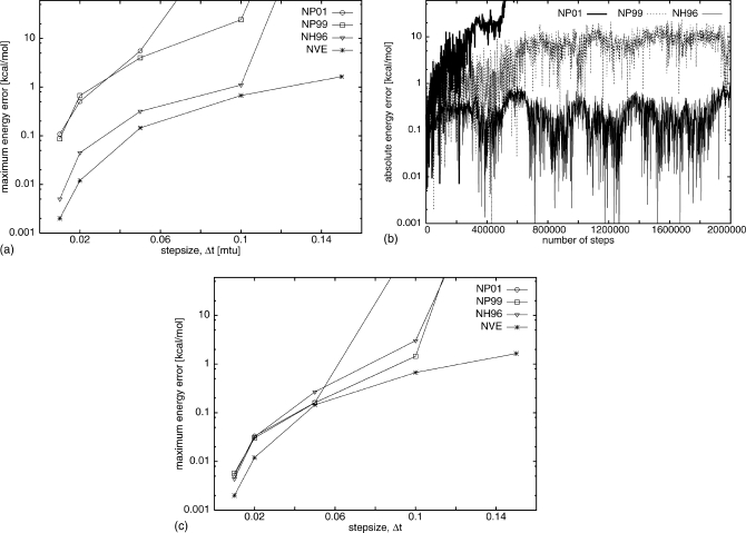
Figure 5a shows the maximum energy error as a function of step size for NH96, NP01, and NP99 for UNRES simulations started from the high-energy extended structure and also for NVE UNRES MD. Errors for NH96 were comparable to those for NVE up to a step size Δt=0.10; for Δt=0.15 only NVE was stable with errors up to 1 kcal∕mol. Both NP01 and NP99 give larger errors for all time steps and are stable up to Δt=0.05 for NP01 but 0.10 for NP99. Details of the simulations for Δt=0.10 are shown in Fig. 5b. Although both NP99 and NH96 are stable, the errors for NP99 are larger and grow over the first half million steps and then stabilize around 10 kcal∕mol. NP01 is not stable, as the errors quickly grow to large values. Figure 5c shows the maximum energy error as a function of step size for NH96, NP01, NP99, and NVE for UNRES simulations started from the pre-equilibrated helical conformation. Errors for NH96 are comparable to those for simulations started from the high-energy extended structure. Both NP01 and NP99 give smaller errors for all time-steps compared to simulations started with the high-energy extended structure but are not stable for larger time steps.
Figure 5.
(a) The maximum absolute energy errors as a function of the step size from the UNRES MD simulations of 20-residue polyglycine starting from the high-energy extended structure for two versions of Nosé–Poincaré (NP01 and NP99) and Nosé–Hoover (NH96) thermostats, and, as a reference, results of microcanonical (NVE) simulations started from the preequlibrated low-energy helical structure. Step sizes range from Δt=0.01 to Δt=0.15; Q=0.5. The maximum absolute energy error is in a logarithmic scale. (b) The absolute energy error as a function of number of steps for Nosé–Poincaré (NP01 and NP99) and Nosé–Hoover (NH96) thermostats at Δt=0.10 for simulations starting from the high-energy extended structure. (c) The maximum absolute energy errors as a function of the step size from the UNRES MD simulations of 20-residue polyglycine starting from the pre-equilibrated low-energy helical structure for two versions of Nosé–Poincaré (NP01 and NP99) and Nosé–Hoover (NH96) thermostats, and microcanonical (NVE) simulations; the other parameters are the same as in (a).
The computational time cost for each thermostat is compared in Table 1. Berendsen is the cheapest and Langevin is the most expensive method. The thermostats in this work are only slightly more expensive than Berendesen, with NP01 the cheapest and NH96 the most expensive. This is reasonable, considering the number of steps taken in each integration scheme (see the Methods section for the algorithms): NP01 has eight steps, NP99 has seven but involves solving a quadratic equation, and NH96 has 12 steps.
Table 1.
Comparison of computational cost. (UNRES MD simulation using Δt=0.05, Q=0.5, for 350 000 steps.)
| Method | Total time (s) |
|---|---|
| Nosé–Poincaré (NP01) | 204 |
| Nosé–Poincaré (NP99) | 207 |
| Nosé–Hoover (NH96) | 217 |
| Langevin | 272 |
| Berendsen | 195 |
RESPA with Lennard-Jones fluid
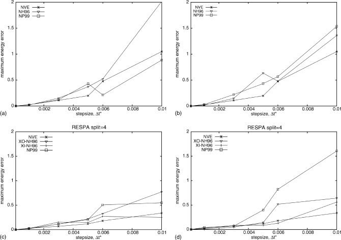
The results reported in Sec. 3A pertain to a high simulation temperature (3000 K or 6 reduced temperature units) at which the system is disordered. However, in our application of the thermostats, we are interested in folded proteins which are ordered systems. We found that, at T=300 K (0.6 reduced temperature units), the Lennard-Jones fluid becomes ordered with particles arranged in rows. The approximate transition temperature is 400 K and the system becomes definitely disordered at 600 K. We, therefore, have examined the NH96 and NP99 thermostats for the Lennard-Jones fluid at 300 K. The maximum absolute error after 500 000 MD steps for runs with the NH96 and NP99 thermostats and for NVE runs as reference are plotted in Fig. 6. The NVE runs were always started from structures equilibrated at T=300 K because they are not thermostated during the course of a run.
Figure 6.
The maximum absolute energy errors as a function of the step size from the Lennard-Jones fluid MD simulations at T=300 K (0.6 reduced temperature units) without RESPA [(a) and (b)] and with RESPA with split=4 [(c) and (d)]. The types of runs are as follows: NVE (stars), NH96 (triangles), and NP99 (squares), and the values of the time step were Δt*=0.001, 0.003, 0.005, 0.006, and 0.01, respectively, for all runs. Runs (a) and (c) were started from a system equilibrated at T=300 K while runs (b) and (d) were started from a system equilibrated at T=600 K.
For runs started from structures equilibrated at T=300 K [Figs. 6a, 6c], introducing RESPA with split=4 improves the performance of the NH96 and NP99 algorithm, as well as of the reference NVE runs. However, when runs are started from higher-temperature and, consequently, a nonequilibrated structure, use of RESPA (with split=4) does not improve the performance of the NP99 algorithm for Δt*>0.004; however, it does for the NH96 algorithm in both the XI (Ref. 12) and XO (Ref. 12) versions.
RESPA with UNRES
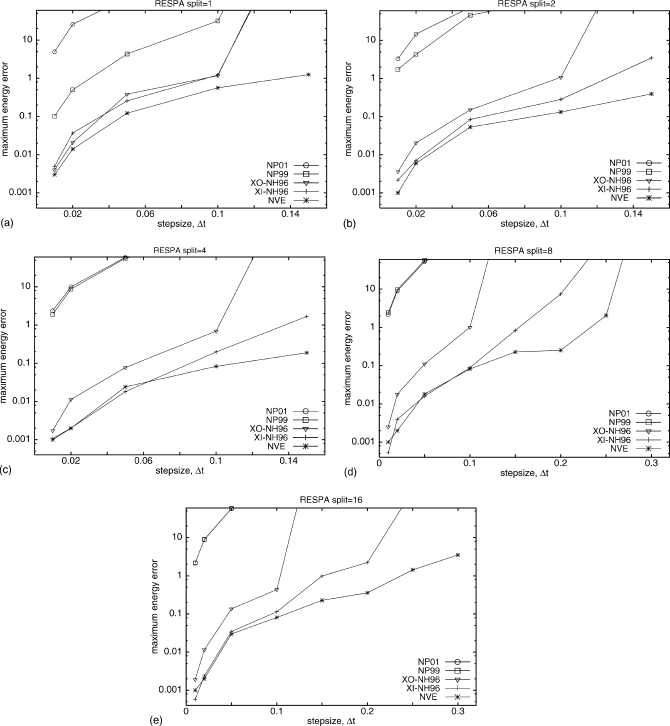
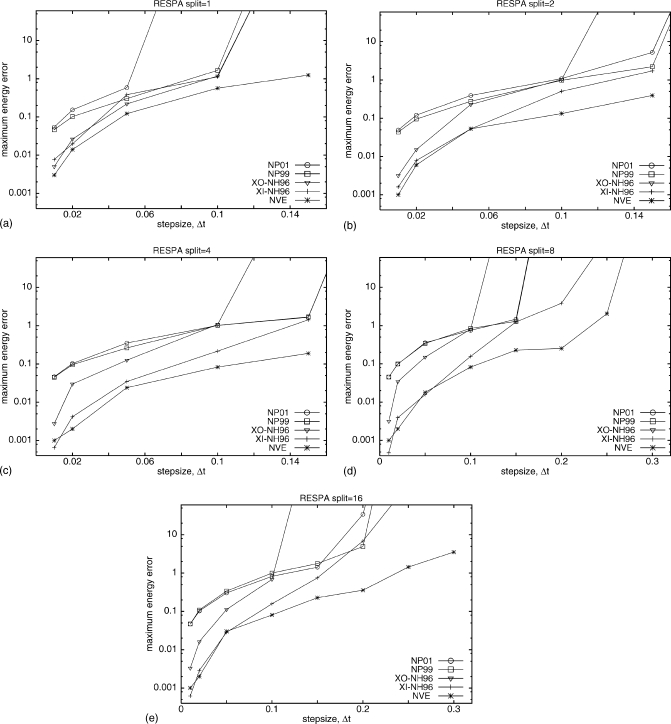
To enable a large step size to be used, multiple-time-step RESPA MD (Ref. 20) runs with Nosé–Hoover [both XI-RESPA and XO-RESPA NH96 (Ref. 12)] and Nosé–Poincaré (NP01 and NP99) thermostats were simulated. Figure 7 shows a comparison of the maximum energy error as a function of step size for different methods and different RESPA splits for simulations started with high-energy extended structure. RESPA with split=1 divides the forces into two groups, fast and slow varying, but does not introduce a time split for the fast-varying forces, and thus should be comparable to UNRES MD simulations [Fig. 5a]. This is the case for all but NP01, which was less stable for RESPA with split=1 than for regular UNRES MD with the same time step. After introducing a time split, both NP99 and NP01 led to large errors for all splits even for small time steps, whereas NH96 is much more stable. XI-RESPA and XO-RESPA NH96 led to comparable errors for split=1, and deviate for larger splits. XI-RESPA NH96 is the most stable method for all splits, with errors only slightly larger than NVE RESPA, which was used as a reference. While it should be true that errors decrease with increasing RESPA split, this was observed only for NH96 and NVE in comparison to regular UNRES MD (i.e., UNRES with no RESPA). Only for XI-RESPA NH96 were significant improvements obtained with RESPA, although RESPA split=16 produced lower errors only for larger time steps compared with RESPA split=8. For the second set of simulations started from the pre-equilibrated helical conformation, the errors for all algorithms were more comparable to each other, as shown in Fig. 8. The errors did not decrease significantly with increasing RESPA split but this increase allows larger time steps for all methods studied when there are no large changes in the potential energy of the simulated system. From a practical point of view, this is less important as thermostats should allow fast equilibration to the desired temperature and should not be sensitive to changes in the potential energy of the system.
Figure 7.
The maximum absolute energy errors as a function of the step size from the UNRES MD simulations with RESPA of 20-residue polyglycine starting from the high-energy extended structure for two versions of Nosé–Poincaré (NP01 and NP99) and Nosé–Hoover (NH96) thermostats and microcanonical (NVE). Nosé–Hoover was run with a XI-RESPA and a XO-RESPA version. Step sizes range from Δt=0.01 to Δt=0.30; Q=0.5. Simulations ran for two million steps. The maximum energy error (y axis) is in a logarithmic scale. (a) RESPA with split=1, for Δt=0.01 to Δt=0.15. (b) RESPA with split=2, for Δt=0.01 to Δt=0.15. (c) RESPA with split=4, for Δt=0.01 to Δt=0.15. (d) RESPA with split=8, for Δt=0.01 to Δt=0.20. (e) RESPA with split=16, for Δt=0.01 to Δt=0.30.
Figure 8.
The maximum absolute energy errors as a function of the step size from the UNRES MD simulations with RESPA of 20-residue polyglycine starting from the pre-equilibrated low-energy helical structure for two versions of Nosé–Poincaré (NP01 and NP99) and Nosé-Hoover (NH96) thermostats and microcanonical (NVE). All parameters are the same as in Fig. 6.
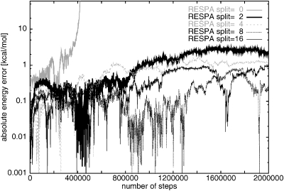
Details of the absolute energy errors as a function of the number of steps for XI-RESPA NH96 RESPA simulations started from the extended structure, at Δt=0.15, are seen in Fig. 9. UNRES MD without RESPA (i.e., split=0) is not stable for such a large time step. Absolute energy errors grow for split=2 and 4, but are still acceptably small. Increase of the time split to 8 makes the errors smaller (oscillating around the constant value, approximately 0.1), but an increase still further to 16 leads to no improvement. RESPA thus allows an increase of the time step to larger values than those used for regular UNRES MD.
Figure 9.
The absolute energy error as a function of number of steps for XI-RESPA Nosé–Hoover (NH96) for Δt=0.15, Q=0.5, and run for two million steps for different RESPA splits. RESPA split=0 indicates UNRES MD simulation without RESPA.
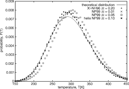
Apart from conservation of the extended energy which serves as a measure of the stability of a run, a feature of interest of the algorithms under consideration is the behavior of the distribution of temperature and other observables, particularly when the extended energy fails to be conserved. The temperature distributions of the 20-residue polyglycine system simulated using UNRES with the NH96 and NP99 thermostats with RESPA (split=8) for various time steps, and starting from either the extended or the equilibrated α-helical structure, are shown in Fig. 10. It can be seen that the temperature distribution for the system run with the NP99 thermostat with Δt=0.05 mtu, in which large nonconservation of the extended energy is observed [Fig. 7d], differs significantly from the theoretical temperature distribution and from the distributions obtained for the other runs in which nonconservation of the extended energy is not so pronounced. On the other hand, the distributions of the radius of gyration and the velocity autocorrelation function do not differ significantly (data not shown).
Figure 10.
Comparison of the temperature distribution obtained for the 20-residue polyglycine system obtained with XI-NH96 started from the extended structure with Δt=0.2 mtu (pluses), NP99 started from the extended structure with Δt=0.01 mtu (x’s), NP99 started from the extended structure with Δt=0.05 mtu (squares), and NP99 started from the equilibrated α-helical structure with Δt=0.1 mtu (stars), all run with RESPA (split=8). The theoretical distribution is of the form , and is plotted with a solid line.
The computational time cost for XI-RESPA NH96 for different splits is compared in Table 2. The increase in computational time is linear since the main cost is the evaluation of the fast-varying forces at additional time steps. Introduction of multiple time steps increases the computational cost, but enables us to use larger integration time steps. The largest possible Δt without RESPA is 0.10 for NH96 and NP01 thermostats (although NP01 leads to much larger errors). Upon introducing RESPA splits, 0.15 is the largest stable time step for split=2 and 4, with errors smaller for split=4. Further increase of RESPA split allows the increase of Δt to 0.20. However, such an increase is not practical due to the increase in computational time cost, as shown in Table 2. Small errors for simulations using Δt=0.20 are produced only with RESPA split=16, which is five times more expensive than regular UNRES MD with Δt=0.10.
Table 2.
Comparison of computational cost for UNRES XI-RESPA. (UNRES MD with RESPA using Δt=0.15, Q=0.5, for 350 000 steps.)
| RESPA split | Total time (s) |
|---|---|
| 2 | 315 |
| 4 | 409 |
| 8 | 586 |
| 16 | 950 |
CONCLUSION
Algorithms for Nosé–Hoover (NH96) and two versions of Nosé-Poincaré (NP01 and NP99) thermostats have been compared for two different model systems: a simple Lennard-Jones fluid, and a 20-residue polyglycine chain modeled with an UNRES force field. All three methods provide the proper velocity and temperature distributions, with Q adjusted depending on the model system. Unexpectedly, when rapid changes of the potential energy occur or for larger time steps, the Nosé–Poincaré algorithm, which has a canonical symplectic structure, gives larger errors for both model systems in the conserved quantity than Nosé–Hoover, which does not have a canonical symplectic structure. This feature is manifested to a moderate extent for the Lennard-Jones fluid for which the energy change when passing to the ordered configuration is smaller, and to a great extent for the 20-residue polyglycine system with UNRES in which the energy drops sharply upon folding. Nosé–Hoover is less stable only for smaller time steps for a Lennard-Jones fluid. For more complicated systems such as the UNRES polypeptide chain, the implementation of the Nosé–Hoover algorithm by Martyna et al.12 and the Nosé–Poincaré algorithm perform comparably when started from equilibrated structures, while the Nosé–Hoover algorithm is always more stable when a nonequilibrated extended structure is used as a starting point. In a recent review, Bond and Leimkuhler analyzed the numerical stability of different integration schemes for Nosé dynamics and also found that there are examples of efficient nonsymplectic integrators.34 They concluded that the advantage of the nonsymplectic Nosé–Hoover algorithm over the symplectic Nosé–Poincaré algorithm is that the former works with a physical momentum variable pi. The Nosé–Poincaré algorithms use the virtual momenta and the thermostat variable s computed at staggered time points which can produce instability when s approaches zero.34 The symplectic structure and the choice of virtual versus physical variables are mostly independent, but both affect the stability of the algorithm.
The greater sensitivity of the Nosé–Poincaré algorithm compared to the Nosé–Hoover algorithm can be explained as follows. In the Nosé–Poincaré Hamiltonian, the potential energy V is multiplied by the variable s. Because V depends only on coordinates and the error in coordinates (including s) is fourth order36 in the time step, the error in the conserved quantity scales as the fourth time derivative of V or Vs for the Nosé–Hoover and Nosé–Poincaré algorithm, respectively. The fourth time derivative of Vs contains all derivatives of V, i.e., even less rapid changes of V will contribute to error.
Introducing Nosé–Hoover (XI-RESPA and XO-RESPA NH96) and Nosé–Poincaré (NP01 and NP99) for multiple-time-step UNRES RESPA MD produced a similar conclusion that Nosé–Hoover is more stable for this model system. Here XI-RESPA NH96 enabled us to increase the integration time step from Δt=0.10 to Δt=0.15. Further increase of the time step is possible only with a detriment to the computational cost; the time split RESPA cost grows linearly with only a slight increase of the largest stable time step. In conclusion, the optimum thermostat for use with UNRES is NH96 with XI-RESPA.
ACKNOWLEDGMENTS
We thank Professor G.S. Ezra for helpful comments on the manuscript. This work was supported by grants from the U.S. National Science Foundation (MCB05-41633), the U.S. National Institutes of Health (GM-14312), the National Institutes of Health Fogarty International Center Grant No. TW007193, and No. DS 8372-4-0138-8 from the Polish Ministry of Science and Higher Education. This research was conducted by using the resources of (a) our 818-processor Beowulf cluster at the Baker Laboratory of Chemistry and Chemical Biology, Cornell University, (b) the National Science Foundation Terascale Computing System at the Pittsburgh Supercomputer Center, and (c) the John von Neumann Institute for Computing at the Central Institute for Applied Mathematics, Forschungszentrum Jülich, Germany.
References
- Alder B. J. and Wainwright T. E., J. Chem. Phys. 10.1063/1.1743957 27, 1208 (1957). [DOI] [Google Scholar]
- Alder B. J. and Wainwright T. E., in Molecular Dynamics by Electronic Copmuters, Transport Processes in Statistical Mechanics, Vol. 97, edited by Prigogine I. (Interscience, New York, 1958), p. 97. [Google Scholar]
- Scheraga H. A., Khalili M., and Liwo A., Annu. Rev. Phys. Chem. 10.1146/annurev.physchem.58.032806.104614 58, 57 (2007). [DOI] [PubMed] [Google Scholar]
- Andersen H. C., J. Chem. Phys. 10.1063/1.439486 72, 2384 (1980). [DOI] [Google Scholar]
- Kubo R., Rep. Prog. Phys. 10.1088/0034-4885/29/1/306 29, 255 (1966). [DOI] [Google Scholar]
- Schneider T. and Stoll E., Phys. Rev. B 10.1103/PhysRevB.17.1302 17, 1302 (1978). [DOI] [Google Scholar]
- Berendsen H. J. C., Postma J. P. M., van Gunsteren W. F., DiNola A., and Haak J. R., J. Chem. Phys. 10.1063/1.448118 81, 3684 (1984). [DOI] [Google Scholar]
- Morishita T., J. Chem. Phys. 10.1063/1.1287333 113, 2976 (2000). [DOI] [Google Scholar]
- Nosé S., J. Chem. Phys. 10.1063/1.447334 81, 511 (1984). [DOI] [Google Scholar]
- Nosé S., Mol. Phys. 10.1080/00268978400101201 52, 255 (1984). [DOI] [Google Scholar]
- Hoover W. G., Phys. Rev. A 10.1103/PhysRevA.31.1695 31, 1695 (1985). [DOI] [PubMed] [Google Scholar]
- Martyna G. J., Tuckerman M. E., Tobias D. J., and Klein M. L., Mol. Phys. 10.1080/00268979650027054 87, 1117 (1996). [DOI] [Google Scholar]
- Bond S. D., Leimkuhler B. J., and Laird B. B., J. Comput. Phys. 10.1006/jcph.1998.6171 151, 114 (1999). [DOI] [Google Scholar]
- Zare K. and Szebehely V., Celest. Mech. 10.1007/BF01650285 11, 469 (1975). [DOI] [Google Scholar]
- Nosé S., J. Phys. Soc. Jpn. 10.1143/JPSJ.70.75 70, 75 (2001). [DOI] [Google Scholar]
- Tuckerman M., Berne B. J., and Martyna G. J., J. Chem. Phys. 10.1063/1.460259 94, 6811 (1991). [DOI] [Google Scholar]
- Tuckerman M., Berne B. J., and Martyna G. J., J. Chem. Phys. 10.1063/1.463137 97, 1990 (1992). [DOI] [Google Scholar]
- Liwo A., Khalili M., and Scheraga H. A., Proc. Natl. Acad. Sci. U.S.A. 10.1073/pnas.0408885102 102, 2362 (2005). [DOI] [PMC free article] [PubMed] [Google Scholar]
- Khalili M., Liwo A., Rakowski F., Grochowski P., and Scheraga H. A., J. Phys. Chem. B 10.1021/jp058008o 109, 13785 (2005). [DOI] [PMC free article] [PubMed] [Google Scholar]
- Rakowski F., Grochowski P., Lesyng B., Liwo A., and Scheraga H. A., J. Chem. Phys. 10.1063/1.2399526 125, 204107 (2006). [DOI] [PubMed] [Google Scholar]
- Swope W. C., Anderson H. C., Berens P. H., and Wilson K. R., J. Chem. Phys. 10.1063/1.442716 76, 637 (1982). [DOI] [Google Scholar]
- Hairer E., Appl. Numer. Math. 10.1016/S0168-9274(97)00061-5 25, 219 (1997). [DOI] [Google Scholar]
- Liwo A., Czaplewski C., Pillardy J., and Scheraga H. A., J. Chem. Phys. 10.1063/1.1383989 115, 2323 (2001). [DOI] [Google Scholar]
- Kubo R., J. Phys. Soc. Jpn. 10.1143/JPSJ.17.1100 17, 1100 (1962). [DOI] [Google Scholar]
- Chinchio M., Czaplewski C., Liwo A., Oldziej S., and Scheraga H. A., J. Chem. Theory Comput. 3, 1236 (2007). [DOI] [PubMed] [Google Scholar]
- Ołdziej S., Kozłowska U., Liwo A., and Scheraga H. A., J. Phys. Chem. A 10.1021/jp0223410 107, 8035 (2003). [DOI] [Google Scholar]
- Liwo A., Ołdziej S., Czaplewski C., Kozłowska U., and Scheraga H. A., J. Phys. Chem. B 10.1021/jp030844f 108, 9421 (2004). [DOI] [Google Scholar]
- Liwo A., Pincus M. R., Wawak R. J., Rackovsky S., Ołdziej S., and Scheraga H. A., J. Comput. Chem. 18, 874 (1997). [DOI] [Google Scholar]
- Ołdziej S., Łagiewka J., Liwo A., Czaplewski C., Chinchio M., Nanias M., and Scheraga H. A., J. Phys. Chem. B 10.1021/jp040329x 108, 16950 (2004). [DOI] [Google Scholar]
- Ołdziej S., Liwo A., Czaplewski C., Pillardy J., and Scheraga H. A., J. Phys. Chem. 108, 16934 (2004). [Google Scholar]
- Liwo A., Khalili M., Czaplewski C., Kalinowski S., Ołdziej S., Wachucik K., and Scheraga H. A., J. Phys. Chem. B 10.1021/jp065380a 111, 260 (2007). [DOI] [PMC free article] [PubMed] [Google Scholar]
- Khalili M., Liwo A., Jagielska A., and Scheraga H. A., J. Phys. Chem. B 10.1021/jp058007w 109, 13798 (2005). [DOI] [PMC free article] [PubMed] [Google Scholar]
- Leimkuhler B. and Reich S., Simulating Hamiltonian Dynamics (Cambridge University Press, Cambridge, England, 2004). [Google Scholar]
- Bond S. D. and Leimkuhler B. J., Acta Numerica 16, 1 (2007). [Google Scholar]
- Barth E., Leimkuhler B., and Sweet C., Lecture Notes in Comp. Science and Eng. 49, 125 (2006). [Google Scholar]
- Frenkel D. and Smit B., Understanding Molecular Simulations. From Algorithms to Applications (Elsevier, New York, 2002), p. 70. [Google Scholar]


