

Abstract
We designed a simple position-specific hidden Markov model to predict protein structure. Our new framework naturally repeats itself to converge to a final target, conglomerating fragment assembly, clustering, target selection, refinement, and consensus, all in one process. Our initial implementation of this theory converges to within 6 Å of the native structures for 100% of decoys on all six standard benchmark proteins used in ROSETTA (discussed by Simons and colleagues in a recent paper), which achieved only 14%–94% for the same data. The qualities of the best decoys and the final decoys our theory converges to are also notably better.
Keywords: protein structure prediction, hidden Markov model, fragment assembly
We wished to find a unified and the simplest model for protein structure prediction, one of the major open problems in science. We were not interested in trying PSI-BLAST for easy targets, threading by RAPTOR (Xu and Li 2003) for harder targets, fragment assembly by ROSETTA (Simons et al. 1997) for ab initio targets, or consensus for everything. We were also not interested in using different methods for different steps, such as Monte Carlo fragment assembly, clustering, selecting, and refinement. Nature does not do this. It does not fit with Occam's razor principle (Li and Vitanyi 1997; Baker 2000).
Nature prefers simplicity. We wished to find one theory, one model, as simple as possible that goes from an input sequence to the final structure. This theory should embody homology modeling, threading, fragment assembly (all stages of it), loop modeling, refinement, side-chain packing, and consensus. The theory must be simple, robust, and effective.
This work presents our initial efforts in building a theory toward this goal and our preliminary implementation of this theory, FALCON, together with clear-cut experimental results. Some ideas of our work come from three lines of research: fragment assembly, hidden Markov model sampling, and Ramachandran basins.
The most successful approach for ab initio structure prediction is to use short structural fragments to model local interactions among the amino acids of a segment and utilize the nonlocal interactions to arrange these short structural fragments to form native-like structures (Simons et al. 1997). Despite the importance of nonlocal interactions in directing the search to discover the native-like protein structures, the relationship between local structures and the interactions among amino acids within a local structure remain active issues of research. An accurate prediction of the local structural bias for a sequence segment is critically important to protein structure prediction.
According to the Levinthal paradox (Levinthal 1968), the number of possible conformations of a protein chain is exponential in the protein sequence length due to the large degrees of freedom of the unfolded polypeptide chain. As a consequence, a brute-force enumeration of all possible conformations for a given sequence is both computationally and physically infeasible. However, the local structural bias information restricts the possible conformations of each sequence segment and therefore narrows down the conformation space of the whole polypeptide chain significantly.
Structural motif is a straightforward description of local structural bias. The idea of structural motif can be traced back to Pauling and Corey (1951), in which a protein fold is modeled as an assembly of smaller building blocks from the regular secondary structure elements. In past years, considerable work (Rooman et al. 1990; Bystroff et al. 1996; Han et al. 1997; Bystroff and Baker 1998; Camproux et al. 1999; Gerard 1999; Li et al. 2008) has been conducted to define local structural motifs and analyze their structural characterization and sequence preferences. The sequence preferences can be used to predict structural motif for new sequences. Another approach is to search for recurrent sequence patterns first and then study the structural motif shared by these recurrent sequence patterns. This approach can identify new structural motifs since the important structural properties need not be specified in advance. HMMSTR (Bystroff et al. 2000), a hidden Markov model on structural motif space, attempted to describe the overlaps of structural motifs and the transition probability between motifs. HMMSTR can be considered as a probabilistic version of a structural motif library.
Structural motifs serve as the foundation to obtain better predictions. For example, ROSETTA (Simons et al. 1997) selected 9-mer structural fragments from known protein structures as building blocks, while TASSER (Zhang et al. 2005; Zhang 2007) generated fragments of various lengths from threading results. Despite the promising progress of fragment assembly methods, the structural motif strategy still suffers from its inherent discrete nature. That is, the structural motif library is discrete while the conformation space of a protein is continuous. Therefore, it is impossible to cover the whole conformation space by a limited number of structural motifs. This drawback limits the accuracy of protein structure prediction (Holmesand and Tsai 2004; Gong et al. 2005).
An alternative way to describe local structural bias is a Ramachandran basin (Ramachandran and Sasisekharan 1968). A Ramachandran basin refers to a specific region of a Ramachandran plot imposed by local interactions among amino acids. A Ramachandran basin provides a convenient way to present the preference of a specific torsion angle. Colubri et al. (2006) employed the Ramachandran basin technique to investigate the levels of representation required to predict protein structure. Specifically, they tested the ability to recover the native structure from a given Ramachandran basin assignment for each amino acid. In this method, the Ramachandran plot is divided into five predetermined Ramachandran basins. By decomposing the Ramachandran plot into four or more basins, Shortle (2002) calculated the propensities of amino acids mapped to each basin. Shortle argued that these propensities are the results of local side-chain–backbone interactions and may restrict the denatured conformation ensemble to a relatively small subset of native-like conformations. Gong et al. (2005) also investigated the protein structure-reconstructing problem from coarse-grained estimation of the native torsion angle. The only difference in these works lies at the definition of a Ramachandran basin: Gong et al. (2005) partitioned both φ and ψ angle intervals into six ranges, each range of 60°; thus, the Ramachandran map is partitioned into 36 basins uniformly. These three studies demonstrate that the knowledge of torsion angles helps the reconstruction of small-size proteins. However, these three works partition the Ramachandran plot into basins in a random manner without statistical explanations describing the torsion angle distributions of each basin. Furthermore, to give each residue a coarse Ramachandran basin assignment, the native structure should be known in advance, which makes these frameworks infeasible for real-life protein structure prediction.
As the third precursor to our work, Hamelryck et al. (2006) proposed to apply FB5, a directional distribution, to parameterize the local structural bias. Using this tool, they investigated the local bias in (θ, τ) space rather than (φ, ψ) space. In this method, the local structural bias for each amino acid is trained via a hidden Markov model called FB5-HMM. Instead of HMM, Xu et al. (see Zhao et al. 2008) proposed a CRFSampler, a protein-structure-sampling framework based on another probabilistic graph model, Conditional Random Fields (Bishop 2006), with improved results. The success of these methods suggests the advantage of continuous torsion angle distributions over discrete structural motifs: Using the torsion angle distribution technique, it is possible to generate conformations with local structures not occurring in the structural fragment library. In addition, experimental results demonstrate that the derived local biases can help to generate native-like conformations and support the view that relatively few conformations are compatible with the local structural biases (Hamelryck et al. 2006).
Despite the promising advancements, the FB5-HMM type of approach has three serious disadvantages. First, FB5-HMM reports the optimal number of local biases as 75 by training on a large set of representative protein structures. In other words, the (φ, τ) map that is used to model the local bias is partitioned into 75 basins. This partition scheme implies that a protein sequence of length n has a conformation space of size O(75n), which is astronomically larger than the estimation of O(1.6n) by Sims and Kim (2006). In addition, it is challenging to select suitable models from these 75 local biases for a particular residue. Second, the derived distributions are general, while a residue may have its specific preference for the distributions and therefore none of the 75 local biases suits it. Third, FB5-HMM is incapable of capturing the relationships among the residues of a local segment. As a consequence, though equipped with an elegant statistical model, FB5-HMM has a much lower prediction accuracy compared to ROSETTA (Hamelryck et al. 2006; Zhao et al. 2008).
The new paradigm
We propose a simple and unified paradigm for protein structure prediction. The plan is to probabilistically sample protein structure conformations compatible with local structural biases for a given protein. The architecture of the model is as below.
For residue i, several cosine models (Mardia et al. 2007) are used to describe the local bias of its torsion angle pair (φ i, ψ i);
a position-specific hidden Markov model (HMM) is used to capture the dependencies among local biases of adjacent residues, based on carefully selected fragments (Simons et al. 1997; Li et al. 2008). This HMM is referred to as Fragment-HMM;5
the Fragment-HMM is used to sample a sequence of torsion angle pairs for the given protein sequence. An energy function is used to evaluate the generated decoys and to direct the sampling process to the better decoys;
the generated decoys are fed back to produce more accurate estimations of local structural biases, a more accurate Fragment-HMM and thus, better decoys. This step is executed iteratively to increase the quality of the final decoys, until convergence.
This model has advantages over existing works as follows:
Our Fragment-HMM model combines the very successful fragment assembly method (Simons et al. 1997) and the elegant FB5-HMM idea (Hamelryck et al. 2006). Rather than using the fragments as building blocks, we use them to produce local bias information. We use the directional distribution to model local biases, and use HMM to explore the dependency among the adjacent residues. Unlike FB5-HMM, our Fragment-HMM is position specific.
Our Fragment-HMM naturally enables step 4 to resample decoys. Immediately, one would observe that this applies to obtaining fragments from a known structure. Thus, this naturally enables homology modeling, threading, refinement (requiring more hidden nodes to model side chains), loop modeling, and consensus, unifying all these approaches under one roof.
Step 4 is similar to that of primal and dual optimization processes. The primal goal is to minimize the energy, which is done by discriminating decoys with an energy function, and the dual process is done via sampling our Fragment-HMM to improve the estimation of torsion angles. Step 4 differs from the traditional fragment assembly methods that end with a population of decoys, some good and some bad. Our model does not stop here, but iterates until convergence.
The search space is narrowed down step by step. Monte Carlo is a popular technique for fragment-assembly-based protein structure prediction. However, Monte Carlo suffers from its low efficiency since it does not explore the characteristics of the search space. Specifically, for a protein of length n, the search space size is O(200n) if each sequence segment has 200 candidate structural motifs. This search space remains unchanged in the whole Monte Carlo search process. In contrast, our Fragment-HMM narrows down the search space after each iteration step since the local structural biases are estimated more and more accurately.
We have implemented this theory in FALCON, Fragment-HMM approximating local bias and consensus. The first concern obviously is if FALCON will actually converge to some native-like decoys. We take all six proteins from the ROSETTA benchmark data used by Simons et al. (1997). FALCON converges 100% to within 6 Å for all six proteins after only four iterations.
In order to make further comparisons to evaluate our model, we remove step 4, the iteration step, from FALCON. Then FALCON still generates significantly better results than ROSETTA for these six proteins. FALCON improves both the percentages of good decoys and the RMSD of the best decoys for five proteins out of six. For three of them, the percentages of good decoys are improved by >80%. Similarly FALCON, without step 4, generates better results than FB5-HMM, by far.
These results suggest that succinct, accurate, and flexible descriptions of local biases can significantly improve the quality of protein structure prediction.
Methods
Parameterizing backbones
A protein backbone of n residues consists of a sequence of atoms: N 1, Cα1, C 1,…, Nn, Cαn, Cn. The backbone conformation is fully specified by bond lengths, bond angles, and torsion angles. Three types of torsion angles are defined: φ i, ψ i, and ω i for each residue except for the C and N termini. The angle ω i is restricted to close to 180° or −180°. Bond lengths and bond angles are nearly constants. Therefore, we can parameterize a protein backbone with torsion angle pairs, i.e., the backbone of a protein of length can be approximately reconstructed from torsion angle pairs (φ 1, ψ 1), …, (φ n, ψ n), assuming φ 1 and ψ n are defined for notation simplicity.
Representing local bias of torsion angle pairs
The local structural bias for residue i is represented by the joint distribution of its torsion angle pair (φ i, ψ i). We use the cosine model, a bivariate von Mises distribution over angular or directional space (Singh et al. 2002; Mardia et al. 2007). The probability density function of the cosine model is specified by five parameters κ 1,κ 2, κ 3, μ, and υ:
where μ is the mean value of φ, υ is the mean value of ψ, and c (κ 1, κ 2, κ 3) is a normalization constant:
 |
in which Ip (κ) is the modified Bessel function of the first kind and order P (Abramowitz and Stegun 1972).
An alternative bivariate circular distribution is the sine model (Singh et al. 2002). Mardia et al. (2007) argued that the cosine model outperforms the sine model due to its ability to fit more closely a larger set of distributions.
Given a set of torsion angle pairs A = {(φ, ψ)}, we utilize a set of M cosine models to parameterize these data. The cosine models are combined into a mixture model, which can be formulated as:
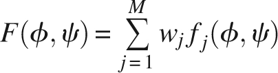 |
where fj, 1 ≤ j ≤ M denotes a cosine model with parameters θ j = (κ j 1,κ j 2,κ j 3,μ j,υ j), wj is the weight of model j with Σj wj = 1. We employ an expectation-maximization (EM) algorithm to derive the most likely estimation of the parameters of the mixture model (Mardia et al. 2007).
The number of cosine models to fit these data is unknown in advance. It is vital to choose a suitable M. Here we use Rissanen's minimum description length (MDL) principle (Li and Vitanyi 1997) to determine the best value for M, i.e., we choose M to minimize the following equation:
where L is the likelihood that M mixture models explain A, and 5 is the number of parameters in each model.
Fragment-HMM: A position specific hidden Markov model
We use an HMM to capture the local dependencies among the adjacent residues. Unlike FB5-HMM, our HMM is position specific, i.e., each residue is associated with a specific subset of hidden nodes and the subset of hidden nodes for all the residues are mutually disjoint.
Model topology
An HMM is a directed graph, where the vertices denote the hidden nodes, and directed edges are used to capture transition and emission probabilities. For each residue i, we obtain a set of possible hidden nodes, denoted as Hi. Given two adjacent hidden node sets Hi and Hi+1, a directed edge <h, h′> is created for each pair of hidden nodes h ∈ Hi and h′ ∈ Hi+ 1. Each possible hidden node (denoted as h) has two types of emissions: a secondary structure type (denoted as S) and a torsion angle pair T = (φ, ψ).
For the ith amino acid, our position-specific HMM describes the following joint probability:
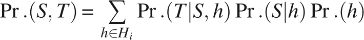 |
where S is the secondary structure type for the ith amino acid and T = (φ, ψ) is its torsion angle pair.
Figure 1 shows an example of Fragment-HMM for five residues. Each residue is associated with a hidden node subset. As illustrated by Figure 1, the hidden node subset H 1 for residue one has two hidden nodes while H 2 for residue two has three possible hidden nodes. Each hidden node is associated with its own cosine model.
Figure 1.

Fragment-HMM: A position-specific hidden Markov model.
Creating hidden nodes
Our HMM is both position and sequence specific. We do not assume we have enough training data available for the target sequences to be predicted. Therefore, the classical Baum–Welch (Baum et al. 1970) method cannot be applied to estimate the parameters. Here, we build the hidden nodes and estimate parameters with a position-specific fragment library, hence the name Fragment-HMM.
The construction process has three steps. First, we parse the target sequence into segments with a sliding window of length l and step size one. In total, there are n − l + 1 segments. We index these sequence segments by 1, 2, …, l. For sequence segment i, we can predict a subset of structural fragments via ROSETTA or FRazor (Li et al. 2008). Since the fragments via FRazor are shown to be better than ROSETTA's fragments (Li et al. 2008), in all experiments in this work, we use only ROSETTA's fragments so that the comparisons are fair. A structural fragment for segment i consists of a predicted torsion angle pair and secondary structure type for each residue from i to n − l + 1. The set of structural fragments is denoted as F. Second, we retrieve all predicted torsion angle pairs for residue i from fragments in F, and use the EM method to generate a set of cosine models. Lastly, for each cosine model, we create a hidden node.
Denote the cosine model specified by hidden node h as mh. The density of mh with parameters (φ, ψ) is written as fh (φ, ψ).
Estimating transition probabilities
We describe the parameter estimation method without considering the secondary structures here for clarity. The secondary structure information is easily integrated into our framework.
The transition probabilities are estimated with fragment library F. Given a fragment q ∈ F and a hidden node h ∈ Hi, we first define the probability that h emits the torsion angle pair predicted by q for residue i as follows:
If q contains a predicted torsion angle pair (φ, ψ) for residue i, we use the value of probability density function fh with parameters (φ, ψ);
otherwise, we define the probability to be 0.
We denote the above probability as gh (q).
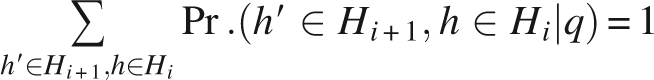
The joint probability Pr.(h′ ∈ Hi +1,h ∈ Hi | q) for edge <h,h′> given fragment q is specified as follows: If a structural fragment q does not contain predicted torsion angles for both residue i and residue i + 1, we let Pr.(h′ ∈ Hi +1, h ∈ Hi | q) = 0; otherwise, we define Pr.(h′ ∈ Hi +1, h ∈ Hi | q) as
 |
The above probability is normalized to ensure
 |
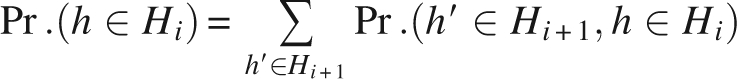
Then, the joint probability Pr.(h′ ∈ Hi +1, h ∈ Hi) can be calculated by
where Pr.(q) can be estimated as the inverse of the number of the fragments in F which contain predicted torsion angle pairs for both residue i and residue i + 1.
Now, we are ready to compute the transition probability Pr.(h′ ∈ Hi +1, | h ∈ Hi) by
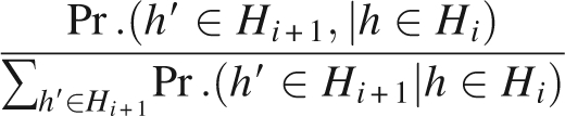 |
The distribution of hidden nodes h ∈ Hi, 1≤ i ≤ n−1 is expressed by
 |
We have specified a Fragment-HMM of order one for simplicity. A Fragment-HMM with higher order can be defined accordingly. We used order-7 and order-2 Fragment-HMM's in FALCON.
Sampling protein structure conformation
Given the position specific Fragment-HMM, to sample a backbone conformation is straightforward.
Sampling hidden nodes
To sample a sequence of hidden nodes, we start by picking up a hidden node from set H1: A node h is picked according to the probability Pr.(h), h ∈ H 1. Given a hidden node h for residue i, we sample a hidden node h′ for residue i + 1, according to the transition probability Pr.(h′ ∈ Hi +1, | h ∈ Hi).
Sampling torsion angle pairs
Then we sample a sequence of torsion angle pairs, one pair per residue according to the cosine model specified by the respective hidden node. A backbone is constructed according to these torsion angles with ideal bond lengths and bond angles. Coupling the angle sampling process, we also sample a sequence of secondary structure types, which is useful for the energy function to evaluate the sampled structure.
Conformation optimization
Similar to the fragment library, for the purpose of fairly testing our theory, we use the energy function of ROSETTA 2.1.0 (released in September 2006).
Initially, we sample a whole sequence of angle pairs and construct a new three-dimensional (3D) backbone structure from these angles. Then we resample a subsequence of torsion angle pairs for a given backbone structure and rebuild a new 3D backbone structure. If the new structure has an energy value better than or equal to that of the previous structure, the new structure is accepted. Otherwise it is accepted with a certain probability by the Metropolis criteria. The process is repeated until the energy is converged or the maximum number of iterations is reached.
Iteratively improving the Fragment-HMM
An energy function directs the generation of a set of decoys. Based on these decoys, some infeasible cosine models may be pruned, and some new cosine models are to be formed. Then these new cosine models can be integrated to build a more accurate Fragment-HMM with refined transition and emission probabilities. In turn, accurate cosine models and HMM will result in better structures.
Therefore, we take a set of generated decoys as a position-specific fragment library and use them as input to regenerate cosine models and a new Fragment-HMM. This way, we generate a set of better decoys. Iterating, more and more accurate cosine models would be obtained, if the energy function biases toward the native-like structures.
Results
FALCON is implemented with C++ on Linux
Data set
We used the six proteins that were used in previous studies (Simons et al. 1997; Kolodny et al. 2002; Hamelryck et al. 2006). They are displayed in Table 1: Protein A (code 1FC2), Homeodomain (code 1ENH), protein G (code 2GB1), Cro repressor (code 2CRO), protein L7/L12 (code 1CTF), and calbidin (code 4ICB).
Table 1.
The number of cosine models per residue

The position-specific fragment library for each protein was obtained from the recently released ROSETTA version 2.1.0. Its structural fragments were selected from a set of 1020 protein chains, which are included in ROSETTA's fragment generation module. We used ROSETTA's energy function and its default settings.
We predict 200 structural fragments for each 9-mer sequence segment of the target protein. The homology proteins of the target sequence are identified by running NCBI-BLAST first (Altschul et al. 1997), and then are removed before we predict the structural fragments. Therefore, we can avoid the possible overlaps between the training and testing sets and make the experiments convincing.
Torsion angle distributions
We derived the most likely torsion angle distributions for each residue of the six proteins. A typical and concrete example for residue 13 of protein 2CRO is plotted in Figure 2A. Figure 2A contains two cosine models, which are centered at (−1.55,−0.28) and (−1.58,2.57). This indicates that the residue has two possible local bias preferences: One corresponds to an α-secondary structure type and the other corresponds to a β-secondary structure type. This is one of the major differences between our Fragment-HMM and FB5-HMM: In FB5-HMM (and CRFSampler) the number of distributions and the corresponding parameters are uniform for all the residues.
Figure 2.

Torsion angle pair distributions and generated protein structure. Panels A–D display the evolution of torsion angle pair distributions for residue 41 of protein 2CRO. The x-axis is φ angle and the y-axis is ψ angle. (A) Iteration 1: Two cosine models centered at (1.55, 0.28) and (1.58, 2.57). (B) Iteration 2: Three cosine models centered at (1.25, 0.52), (1.75, 1.26), and (1.82, 0.07). (C) Iteration 3: Two cosine models centered at (1.22, 0.44) and (1.82, 0.09). (D) Iterations 4 and 5: One cosine model centered at (1.86, 0.13), and then to (1.86, 0.13) in iteration 6. (E,F) The native structure and the best decoy predicted by FALCON, respectively. The RMSD is 0.557 Å.
Table 1 lists the average number of cosine models per residue for the six proteins generated from the fragment library. These proteins average 1.66 cosine models per residue. Most residues have no more than two cosine models. This observation confirms the fact that for a protein relatively few conformations are compatible with the local biases of all residues. Interestingly, the number of possible conformation clusters, C, is estimated to be C = 1.6n (Sims and Kim 2006), which is consistent with the estimations given by Tendulkar et al. (2005) and Dill (1985), coinciding with our study here. There are several different estimations: According to the Levinthal paradox (Levinthal 1968), the conformational space has a size at least C = 3n (Zwanzig et al. 1992); the number of possible conformation clusters can be estimated to be C = 4n via decomposing the Ramachandran map into four basins (Ramachandran and Sasisekharan 1968; Shortle 2002), and Hamelryck et al. (2006) assigned 75 possible states for every amino acid by decomposing the (θ, τ) plane, which implies a conformation space of size C = 75n. Compared with these estimations, our estimation is drastically smaller. This observation suggests that (1) local structural biases can be accurately described and captured and (2) the conformation space to be searched is greatly reduced, and thus it may be possible to sample a native-like structure from a space where the conformations are compatible with the derived local biases.
Local bias representation: Fragment-HMM versus structural fragments
Local structural biases can be described by structural fragments, or Fragment-HMM with cosine models. We now investigate which approach is better in representing local bias for generating decoys. To answer this question, we compare FALCON, without step 4, and ROSETTA (version 2.1.0) in terms of the percentage of good decoys (<6 Å to the native structure) and RMSD values of the best decoys. To do a fair evaluation, we used ROSETTA's energy function for both programs. The input fragment libraries are generated by ROSETTA and are identical for both programs.
In this experiment, 1000 decoys are generated for each protein, by each of ROSETTA and FALCON. Six angstroms are used as the cutoff value for good decoys. The same criteria are used by Hamelryck et al. (2006). Since the decoys for ROSETTA and FALCON are generated independently, the percentage of good decoys is not expected to fluctuate too much when more decoys are generated.
Observing Table 2, FALCON generates significantly more good decoys than ROSETTA. FALCON improves the percentage of good decoys for 1FC2, 2GB1, 2CRO, 1CTF, and 4ICB, five out of six proteins. Especially for 2GB1, 1CTF, and 4ICB, the improvements are from 53.7%, 14.3%, and 19.9% to 93.4%, 25.6%, and 46.3%, respectively. The quality of the best decoys for these five proteins, 1FC2, 2GB1, 2CRO, 1CTF, and 4ICB, are improved too. We display in Figure 2E a structure with a RMSD of only 0.557 Å to the native structure for 1CTF.
Table 2.
Decoy quality of ROSETTA and FALCON

While one of the roots of our Fragment-HMM was FB5-HMM (Hamelryck et al. 2006), Fragment-HMM has shed its skin to evolve into a significantly stronger model. FB5-HMM describes local biases by using 75 basins in the (θ, τ) plane, while FALCON uses only 1.66 basins on average. Under admittedly different conditions, for the same six proteins in Table 2 and in that order, FB5-HMM (Hamelryck et al. 2006) reports the best decoy accuracies to be 2.6 Å, 3.8 Å, 5.9 Å, 4.1 Å, 4.1 Å, and 4.5 Å, respectively, and good decoy percentages (<6 Å), 17.1%, 12.1%, 0.001%, 1.09%, 0.35%, and 0.38%, respectively, from 100,000 decoys.
FALCON: Zero in on the native structure
We use the cosine model to describe the local bias and use energy function to capture global interactions. Energy function directs the search to discover native-like structures. Hence, energy function may help to reshape the local biases. This conjecture has led to step 4 of FALCON: Feed back the decoys as new positive-specific fragments and iterate. The results are pleasing and illustrative.
Six iterations are executed for each protein, and 1000 decoys are generated at each iteration per protein. The first iteration takes as input the position specific fragment libraries from ROSETTA. The (i + 1)th iteration takes the set of decoys generated by the ith iteration as input.
Table 3 displays the RMSD values of the decoys over the iterations for protein 2CRO. We observe that the RMSDs are converging. After five iterations, the RMSD values of 94.9% of the decoys converge to the range of 3 to 4 Å. Both the best and the worst decoys disappear over the iterations. However, the best decoys diminish far more slowly than the worst decoys. The decoy RMSD distributions for other proteins exhibit similar trends.
Table 3.
RMSD distribution over iterations for protein 2CRO

Figure 2 shows the evolution of torsion angle pair distributions for residue 41 of protein 2CRO. Initially, the torsion angle pairs acquired from structural fragments display two clusters: One lies at the β-strand area, and the other lies at the α-helix area, both initially wrong. Interestingly, the subsequent iterations tend to correct the torsion angle distributions step-by-step.
At the second iteration, the initial two clusters are diminishing, and a new cluster centered at (−1.82,−0.07) emerges. At the third iteration, the β-strand distribution disappears completely, and the new cluster becomes dominant. Next the α-helix distribution disappears at the fourth iteration. In the fifth and sixth iterations, the new cluster becomes denser and denser. Finally, we obtain a distribution centered at (−1.86,−0.13) after six iterations. Notice that there is a small gap between the center of this distribution and the native torsion angle pair (−1.44,−0.63). This gap is inevitable since we adopted the standard bond lengths and bond angles in our structure-generating model (Holmesand and Tsai 2004).
Percentage of good decoys
Table 4 displays the percentages of good decoys, which increase steadily with iterations. All six proteins reach 100% of good decoys after four iterations. In particular, the percentage of good decoys for 1CTF and 4ICB is boosted up to 100% from 25.6% and 46.3%, respectively.
Table 4.
Percentage of good decoys with RMSD below 6 Å after each iteration

Quality of the final reported decoys
The Fragment-HMM is not only used to sample decoys but it is also used to rank a given decoy. We rank each decoy from the fifth iteration according to the probability that the Fragment-HMM generates the decoy and outputs the decoy with the highest probability as FALCON's prediction. Table 5 displays the comparison of FALCON with ROSETTA. ROSETTA's results are obtained by the ROSETTA's clustering program with the default configuration.
Table 5.
Quality of the final reported decoys of ROSETTA and FALCON

As illustrated in Table 5, for five of the six benchmark proteins, 1FC2, 1ENH, 2CRO, 1CTF, and 4ICB, FALCON's final predictions are better than that of ROSETTA, under the RMSD metric. For protein 2GB1, ROSETTA reports a better prediction than FALCON.
We have done further experiments on eight larger proteins with over 100 residues. These proteins are selected from CASP7 free modeling targets (The 7th Critical Assessment of Techniques for Protein Structure Prediction). As shown in Table 6, for five of the eight proteins, i.e., T0283, T0350, T0354, T0361, and T0373, FALCON shows better performance than ROSETTA under the RMSD metric. For example, for target protein T0361 with 169 residues, ROSETTA reports a decoy with a RMSD of 20.009 Å while FALCON reports a decoy with a RMSD of 12.225 Å.
Table 6.
Quality of the final reported decoys of ROSETTA and FALCON on eight larger CASP-7 free-modeling targets

Conclusion
Based on the belief that the simplest theories and models are the better ones, we set out to look for a simple, clean, and unified theoretical model with which we can compute the protein structures.
We have proposed such a theory, based on several previous ideas including the fragment assembly method and hidden Markov model sampling. Our new Fragment-HMM overcomes the difficulties of stiff structural fragments in the sequence assembly approach and the high dimensionality problem in the simple HMM approach. We have implemented our theory and produced clear-cut results. With the iteration technique that is enabled by our Fragment-HMM, we have unified the procedures of fragment assembly, clustering, and final decoy selection.
Ideally, the quality of decoys should converge to its native structure over iterations. However, we notice that, for example, the RMSD values of the decoys for 2CRO converge to 3 Å–4 Å. We believe that the main reason is due to the lack of an accurate energy function at the backbone level to direct the search process and an all-atom energy function for a refinement process. Another reason might be that we have used the idealized bond angle and bond length. This problem can be modeled into our model as well, allowing the sampling program to sample different bond angles and bond lengths as well.
The new model also conveniently embodies other approaches such as homology modeling, threading, loop modeling, refinement, and consensus. We will also integrate our own FRazor fragment library (Li et al. 2008) to improve accuracy. These projects are under way.
Acknowledgments
We thank David Baker and his ROSETTA group for developing and allowing us use of the ROSETTA program. We also thank Dr. Yang Zhang for helpful discussions. This work was made possible by the facilities of the Shared Hierarchical Academic Research Computing Network (SHARCNET: www.sharcnet.ca). This work has been supported by an NSERC grant OGP0046506, the Canada Research Chair program, and MITACS. D.B. acknowledges partial supported from an NSF of China grant (60496324) and a Chinese Government Scholarship.
Footnotes
Reprint requests to: Ming Li, David R. Cheriton School of Computer Science, University of Waterloo, Waterloo, ON N2L 3G1, Canada; e-mail: mli@cs.uwaterloo.ca; fax: 1-519-885-1208; or Jinbo Xu, Toyota Technological Institute at Chicago, Chicago, IL 60637, USA; e-mail: j3xu@tti-c.org; fax: 1-773-834-9881.
Article and publication are at http://www.proteinscience.org/cgi/doi/10.1110/ps.036442.108.
In this paper, in order to obtain strictly fair comparisons, we did not use the fragments of FRazor (Li et al. 2008). We uniformly used the ROSETTA fragments.
References
- Abramowitz, M., Stegun, I.A. Handbook of mathematical functions with formulas, graphs, and mathematical tables. Dover; New York: 1972. [Google Scholar]
- Altschul, S.F., Madden, T.L., Schaffer, A.A., Zhang, J., Zhang, Z., Miller, W., Lipman, D.J. Gapped blast and psi-blast: A new generation of protein database search programs. Nucleic Acids Res. 1997;25:3389–3402. doi: 10.1093/nar/25.17.3389. [DOI] [PMC free article] [PubMed] [Google Scholar]
- Baker, D. A surprising simplicity to protein folding. Nature. 2000;405:39–42. doi: 10.1038/35011000. [DOI] [PubMed] [Google Scholar]
- Baum, L., Petrie, T., Soules, G., Weiss, N. A maximization technique occurring in the statistical analysis of probabilistic functions of Markov chains. The Annals of Mathematical Statistics. 1970;41:164–171. [Google Scholar]
- Bishop, C.M. Pattern recognition and machine learning. Springer; New York: 2006. [Google Scholar]
- Bystroff, C., Baker, D. Prediction of local structure in proteins using a library of sequence-structure motifs. J. Mol. Biol. 1998;281:565–577. doi: 10.1006/jmbi.1998.1943. [DOI] [PubMed] [Google Scholar]
- Bystroff, C., Simons, K., Han, K., Baker, D. Local sequence-structure correlations in proteins. Curr. Opin. Biotechnol. 1996;7:417–421. doi: 10.1016/s0958-1669(96)80117-0. [DOI] [PubMed] [Google Scholar]
- Bystroff, C., Thorsson, V., Baker, D. HMMSTR: A hidden Markov model for local sequence-structure correlations in proteins. J. Mol. Biol. 2000;301:173–190. doi: 10.1006/jmbi.2000.3837. [DOI] [PubMed] [Google Scholar]
- Colubri, A., Jha, A.K., Shen, M.Y., Sali, A., Berry, R.S., Sosnick, T.R., Freed, K.F. Minimalist representations and the importance of nearest neighbor effects in protein folding simulations. J. Mol. Biol. 2006;363:835–857. doi: 10.1016/j.jmb.2006.08.035. [DOI] [PubMed] [Google Scholar]
- Camproux, A., Tuffery, P., Chevrolat, J., Boisvieux, J., Hazout, S. Hidden Markov model approach for identifying the modular framework of the protein backbone. Protein Eng. 1999;12:1063–1073. doi: 10.1093/protein/12.12.1063. [DOI] [PubMed] [Google Scholar]
- Dill, K. Theory for the folding and stability of globular proteins. Biochemistry. 1985;24:1501–1509. doi: 10.1021/bi00327a032. [DOI] [PubMed] [Google Scholar]
- Gerard, J. Recognition of spatial motifs in protein structures. J. Mol. Biol. 1999;285:1887–1897. doi: 10.1006/jmbi.1998.2393. [DOI] [PubMed] [Google Scholar]
- Gong, H., Fleming, P., Rose, G. Building native protein conformation from highly approximate backbone torsion angles. Proc. Natl. Acad. Sci. 2005;102:16227–16232. doi: 10.1073/pnas.0508415102. [DOI] [PMC free article] [PubMed] [Google Scholar]
- Hamelryck, T., Kent, J., Krogh, A. Sampling realistic protein conformations using local structural bias. PLoS Comput. Biol. 2006;2:e131. doi: 10.1371/journal.pcbi.0020131. [DOI] [PMC free article] [PubMed] [Google Scholar]
- Han, K., Bystroff, C., Baker, D. Three-dimensional structures and contexts associated with recurrent amino acid sequence patterns. Protein Sci. 1997;6:1587–1590. doi: 10.1002/pro.5560060723. [DOI] [PMC free article] [PubMed] [Google Scholar]
- Holmesand, J., Tsai, J. Some fundamental aspects of building protein structures from fragment libraries. Protein Sci. 2004;13:1636–1650. doi: 10.1110/ps.03494504. [DOI] [PMC free article] [PubMed] [Google Scholar]
- Kolodny, R., Koehl, P., Guibas, L., Levitt, M. Small libraries of protein fragments model native protein structures accurately. J. Mol. Biol. 2002;323:297–307. doi: 10.1016/s0022-2836(02)00942-7. [DOI] [PubMed] [Google Scholar]
- Levinthal, C. Are there pathways for protein folding? J. Chim. Phys. 1968;65:44–45. [Google Scholar]
- Li, M., Vitanyi, P. An introduction to Kolmogorov complexity and its applications. Springer; New York: 1997. [Google Scholar]
- Li, S.C., Bu, D., Xu, J., Gao, X., Li, M. Designing succinct structural alphabets. Bioinformatics. 2008;24:il82–il89. doi: 10.1093/bioinformatics/btn165. [DOI] [PMC free article] [PubMed] [Google Scholar]
- Mardia, K., Taylor, C., Subramaniam, G. Protein bioinformatics and mixtures of bivariate von Mises distributions for angular data. Biometrics. 2007;63:505–512. doi: 10.1111/j.1541-0420.2006.00682.x. [DOI] [PubMed] [Google Scholar]
- Pauling, L., Corey, R. The pleated sheet, a new layer configuration of polypeptide chains. Proc. Natl. Acad. Sci. 1951;37:251–256. doi: 10.1073/pnas.37.5.251. [DOI] [PMC free article] [PubMed] [Google Scholar]
- Ramachandran, G., Sasisekharan, V. Conformation of polypeptides and proteins. Advan. Prot. Chem. 1968;23:283–438. doi: 10.1016/s0065-3233(08)60402-7. [DOI] [PubMed] [Google Scholar]
- Rooman, M., Rodriguez, J., Wodak, S. Automatic definition of recurrent local structure motifs in proteins. J. Mol. Biol. 1990;213:327–336. doi: 10.1016/S0022-2836(05)80194-9. [DOI] [PubMed] [Google Scholar]
- Shortle, D. Composites of local structure propensities: Evidence for local encoding of long-range structure. Protein Sci. 2002;11:18–26. doi: 10.1110/ps.ps.31002. [DOI] [PMC free article] [PubMed] [Google Scholar]
- Simons, K., Kooperberg, C., Huang, E., Baker, D. Assembly of protein tertiary structures from fragments with similar local sequences using simulated annealing and Bayesian scoring functions. J. Mol. Biol. 1997;268:209–225. doi: 10.1006/jmbi.1997.0959. [DOI] [PubMed] [Google Scholar]
- Sims, G.E., Kim, S.-H. A method for evaluating the structural quality of protein models by using higher-order ϕ-ψ pairs scoring. Proc. Natl. Acad. Sci. 2006;103:4428–4432. doi: 10.1073/pnas.0511333103. [DOI] [PMC free article] [PubMed] [Google Scholar]
- Singh, H., Hnizdo, V., Demchuk, E. Probabilistic model for two dependent circular variables. Biometrika. 2002;89:719–723. [Google Scholar]
- Tendulkar, A.V., Sohoni, M.A., Ogunnaike, B., Wangikar, P.P. A geometric invariant-based framework for the analysis of protein conformational space. Bioinformatics. 2005;18:3622–3628. doi: 10.1093/bioinformatics/bti621. [DOI] [PubMed] [Google Scholar]
- Xu, J., Li, M. Assessment of RAPTORs linear programming approach in CAFASP3. Proteins. 2003;53:579–584. doi: 10.1002/prot.10531. [DOI] [PubMed] [Google Scholar]
- Zhang, Y. Template-based modeling and free modeling by I-TASSER in CASP7. Proteins. 2007;(Suppl 8):108–117. doi: 10.1002/prot.21702. [DOI] [PubMed] [Google Scholar]
- Zhang, Y., Arakaki, A., Skolnick, J. TASSER: An automated method for the prediction of protein tertiary structures in CASP6. Proteins. 2005;61:91–98. doi: 10.1002/prot.20724. [DOI] [PubMed] [Google Scholar]
- Zhao, F., Li, S.C., Sterner, B.W., Xu, J. Discriminative learning for protein conformation sampling. Proteins. 2008;73:228–240. doi: 10.1002/prot.22057. [DOI] [PMC free article] [PubMed] [Google Scholar]
- Zwanzig, R., Szabo, A., Bagchi, B. Levinthal's paradox. Proc. Natl. Acad. Sci. 1992;89:20–22. doi: 10.1073/pnas.89.1.20. [DOI] [PMC free article] [PubMed] [Google Scholar]