An experimental study on the noise properties of X-ray CT sinogram data in Radon space

Abstract

Computed tomography (CT) has been well established as a diagnostic tool through hardware optimization and sophisticated data calibration. For screening purposes, the associated X-ray exposure risk must be minimized. An effective way to minimize the risk is to deliver fewer X-rays to the subject or lower the mAs parameter in data acquisition. This will increase the data noise. This work aims to study the noise property of the calibrated or preprocessed sinogram data in Radon space as the mAs level decreases. An anthropomorphic torso phantom was scanned repeatedly by a commercial CT imager at five different mAs levels from 100 down to 17 (the lowest value provided by the scanner). The preprocessed sinogram datasets were extracted from the CT scanner to a laboratory computer for noise analysis. The repeated measurements at each mAs level were used to test the normality of the repeatedly measured samples for each data channel using the Shapiro-Wilk statistical test merit. We further studied the probability distribution of the repeated measures. Most importantly, we validated a theoretical relationship between the sample mean and variance at each channel. It is our intention that the statistical test and particularly the relationship between the first and second statistical moments will improve low-dose CT image reconstruction for screening applications.

I. Introduction

Computed tomography (CT), performing image reconstruction from Radon space measurement, has been well established as a diagnostic modality through hardware optimization and sophisticated data calibration (Herman 1980). However, clinical use of CT frequently exposes the patients to high X-ray radiation (Linton et al 2003). For screening and image-guided interventional purposes, the associated X-ray exposure risk to the subjects and operators should be minimized. An effective way to minimize the risk is to deliver less X-rays to the subject or decrease the mAs value in the data acquisition protocol to a level as low as achievable for a concerned clinical task. As the mAs value decreases, the noise level of the calibrated data increases and is the underlying fundamental problem.

The noise is introduced during X-ray generation from the X-ray source and then propagates along as X-rays traverse the body and pass through the detection system (Macovski 1982). The detected counts reflect the transmitted X-ray photon numbers and their energies. Studying the noise properties of the transmitted data is currently an attractive research topic (Whiting et al 2006). To reconstruct an acceptable quality image, the transmitted data must be calibrated. While most of the calibration operations are system specific, a mathematical logarithm transform which converts the transmitted data into Radon space is common to all CT systems (Macovski 1982, Whiting et al 2006). Hereafter, the system calibrated and logarithm transformed data is referred to as the preprocessed sinogram or simply sinogram. This work aims to study the noise property of the sinogram as the mAs value decreases. It is expected that the acquired knowledge on the noise properties could improve the well-established Radon-space CT image reconstruction methodologies (Herman 1980) and lead to minimized X-ray exposure risk in clinical applications.

II. Theory

While the noise propagation through detection and calibration operations is a complicated process, the noise distribution at the X-ray generation stage can be expressed as a Poisson functional (Macovski 1982). Consider the polyenergetic nature of X-ray generation where the Poisson function becomes a compound Poisson form which includes a convolution with the X-ray energy spectrum (Snyder et al 1991, Whiting et al 2006). The convolution operation may alter the Poisson distribution (Snyder et al 1991). Additional calibration operations including the logarithm transform can further alter the Poisson distribution (Lu et al 2001, Whiting et al 2006). The data mean remains unaltered, however, the variance changes noticeably as the noise propagates through these calibration operations (Lu et al 2001, 2002, Li et al 2004, Whiting et al 2006). In the following, we will focus on the mean-variance relationship of the Poisson distribution of the transmitted data in Radon space and present a modified mean-variance functional formula which accommodates the variance variation due to the preprocessing calibration operations and other factors, such as bowtie attenuating filtration. A major reason for focusing on the mean-variance relationship is because these first and second statistical moments play an essential role in noise treatment for low-dose CT applications.

2.1. Statistical Distributions of Emitted and Transmitted X-ray Photons

The emission of photons from the X-ray source is a Poisson process with probability given by (Macovski 1982):

$$P_k\left(N_0\right)=\frac{{\left(N_0\right)}^k{e}^{-N_0}}{k!}$$ (1)

where P_k is the probability, in a given time interval, of emitting k photons, and N₀ is the average number of photons emitted during that interval. The process of photon transmission through the body is described by a binary process where photons are either removed or transmitted. This process can be described by a binomial model in which the probability prob of a photon being transmitted is exp(−∫μ ds) and the probability of a photon being removed is 1- prob, where μ represents the linear attenuation coefficient and ds indicates a length element along the photon path (Macovski 1982). It has been shown that the cascading of the Poisson and binomial distributions results in a Poisson distribution (Macovski 1982), i.e., the exit or transmitted photons from the body continue to be Poisson distributed with the rate scaled by the transmission probability prob = exp(−∫μ ds) . Hereafter p = ∫μ ds is called line integral of the attenuation coefficients.

2.2. Mean and Variance of the Line Integral

It has been shown that the mean of the transmitted photon number is a nonlinear function of the line integral of the attenuation coefficient, i.e., N_d = N₀ exp(−∫μ ds) (Macovski 1982). Ideally, the line integral at the detector bin or data channel i can be calculated by:

$$p_i=\ln \frac{N_0}{\kappa }=\ln N_0-\ln \kappa$$ (2)

where κ is a random variable representing the number of transmitted photons at that channel and it follows a Poisson distribution with the mean value N_d . Therefore the measured line integral p_i will also be a random variable. By the use of the Taylor expansion, it has been shown in (Macovski 1982) that the mean p̄_i and variance ${\sigma }_{p_i}^2$ of p_i are given respectively by:

$${\stackrel{‒}{p}}_i=\ln (N_0∕N_d)$$ (3)

$${\sigma }_{p_i}^2=1∕N_d.$$ (4)

Therefore the relationship between the mean and variance of the line integral can be described by the following formula:

$${\sigma }_{p_i}^2=\frac{1}{N_0}\exp \left({\stackrel{‒}{p}}_i\right).$$ (5)

Because of the use of the bowtie attenuating filtration on the X-rays before they arrive at the body, the average number N₀ of photons emitted from the X-ray source will be altered to be dependent on the detector bin position across the field-of-view (FOV), and correspondingly equation (5) becomes:

$${\sigma }_{p_i}^2=\frac{1}{N_{0i}}\exp \left({\stackrel{‒}{p}}_i\right).$$ (6)

where N_0i represents the average photon number just before entering the body and going toward detector bin i, and could be measured in the absence of the body in the FOV, i.e., by an empty scan.

To accommodate deviation from the Poisson distribution due to the polyenergetic nature of X-ray generation and the necessary data calibration operations, the mean-variance relationship (6) could be replaced by (Li et al 2004):

$${\sigma }_{p_i}^2=f_i\exp ({\tilde{p}}_i∕\eta )$$ (7)

where p̃_i = η p̄_i and η is a scaling parameter which enables the measured photon energies to be stored as integers while retaining the dynamic range of the line integrals of the attenuation coefficients. It is system specific, and different CT manufacturers may choose different η values. For example, η is 2294.5 for Siemens CT scanners so that the sinogram data can be saved as a type of two-byte integers for computer manipulations. Notation f_i in equation (7) represents an adjustable factor adaptive to each detector bin i. It mainly considers different incident photon numbers N_0i at different detector bins due to the bowtie attenuating filtration. The magnitude of f_i is primarily determined by the mAs value (which reflects the output photon flux density N₀ from the X-ray source). At a specific mAs level, the values of f_i at different detector bins are mainly affected by the bowtie attenuating filtration across the FOV. Some small variation among neighboring f_i values may reflect the bin-by-bin calibration operations on the uniformity of X-ray generation and detector-bin response. It is also system specific, and its dependence on index i is mainly due to the bowtie filtration and bin-by-bin calibration. Both the parameters η and f_i are object-independent because their theoretical basis is equation (5), which is derived without any assumption about the object. Their values can be completely determined given the CT system settings. In the following, we will study the noise properties of the sinogram by repeated scans of an anthropomorphic torso phantom with the focus on the validation of the mean-variance relationship (7).

III. Experimental Phantom Results

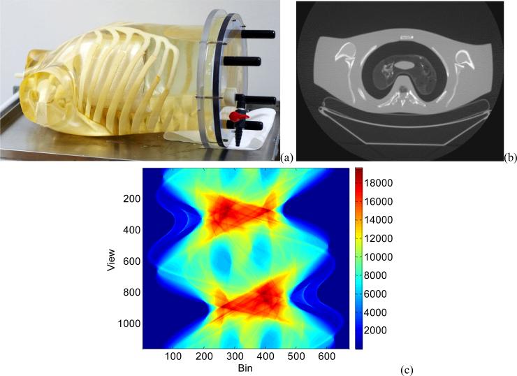
Repeated phantom experiments were performed using a Siemens SOMATOM Sensation16 CT scanner and an anthropomorphic torso phantom of Figure 1 (Radiology Support Devices, Inc., Long Beach, CA). The multi-slice Siemens scanner contains 16 detector rows and each of the 16 detector rows has a z-axis dimension of 0.75 mm. The data acquisition protocols included a tube voltage of 120 kVp, and rotation speed of 0.5 seconds per rotation. A total of five different mAs values were chosen from 100 down to 17 (the lowest provided by the CT scanner): 100, 80, 60, 40, and 17 mAs. At each mAs value, the CT scanner revolved 150 times around the phantom in the step-and-shoot mode at a fixed bed position. Each rotation included 1160 projection views evenly spaced on a circular orbit. Each view contained 672 data elements each from one of the 672 detector bins. The detector arrays in each row were on an arc concentric to the X-ray source with a distance of 1040 mm. The distance from the rotation center to the X-ray source was 570 mm. The detector bin spacing was 1.407 mm. The scaling parameter η is 2294.5 for the Siemens CT system. The measurements were calibrated by the CT system and outputted as the scaled line integrals, which are two-byte integers.

Figure 1.

Illustration of an anthropomorphic torso phantom (a), a CT image of a transverse cross section of the torso phantom (b), and an acquired sinogram data from the transverse cross section (c).

From the 150 repeated scans at each mAs value, we calculated the sample mean p̃_i and variance ${\sigma }_{p_i}^2$ of each channel for one of the 16 detector rows using the outputted two-byte integers. There were a total of 672×1160 channels. Given the calculated pair {p̃_i, ${\sigma }_{p_i}^2$}, we first made a plot on the log variance ln(${\sigma }_{p_i}^2$) against the mean p̃_i for a detector bin at the 1160 view angles (i.e., f_i would be a constant for the 1160 view angles). The plotted curve was nearly a straight line (the r-value from the linear fitting is larger than 0.96), as expected by the following equation:

$$\ln \left({\sigma }_{p_i}^2\right)=\ln \left(f_i\right)+{\tilde{p}}_i∕\eta$$ (8)

and the slope reflects the value of η . Similar plots were obtained for other detector bins and also from projection data of a different commercial (GE HiSpeed four-slice) CT scanner (Li et al 2004). By fitting the plot to a straight line, the slope was approximated as an integer of 2200, which is very close to the true value of 2294.5 provided by the Siemens CT manufacturer (i.e., a small difference of 4%). In the following calculations, the true value of η = 2294.5 was used.

Given the calculated pair {p̃_i, ${\sigma }_{p_i}^2$} and the scaling parameter η of 2294.5, the value of f_i was computed according to equation (7). At each projection view, we calculated the value f_i for each of the 672 detector bins. Figure 2(a) shows the calculated values {f_i} from all the 672×1160 channels (i.e., 672 detector bins and 1160 projection views) at 100 mAs level. It can be observed that each horizontal profile f_i of the 672 bins (across the FOV) has a nearly identical shape at all the 1160 views. Several little curly lines along the view (vertical) direction are seen, this is due to the edges in the phantom sinogram as shown in Figure 1(c). Figure 2(b) shows the curves {f_i} averaged over the 1160 projection views at the five different mAs values. It can be observed that the shapes of the curves are similar at different mAs levels. The shape is also similar to the result in the absence of an object in the FOV as shown in (Whiting et al 2006), where the curve shape is mainly caused by the bowtie filtration used for attenuating the incident X-ray beams across the FOV. It can also be observed that small spikes are present along the curve of f_i regularly spaced across the FOV. This phenomenon is mainly caused by the transition from one small detector module to the next module. These small modules make a curved array of the detector row. If the detector row is made by a single crystal, not an array of small elements, the spikes would be smaller or even disappear. An additional possible cause may be due to a small mismatch of the starting angles of the 150 repeated scans, even though each scan was specified at the same protocol parameters. The chance of this additional possible cause is very small because each of the curves is an average from 1160 views and there are 150 repeated scans at each view.

Figure 2.

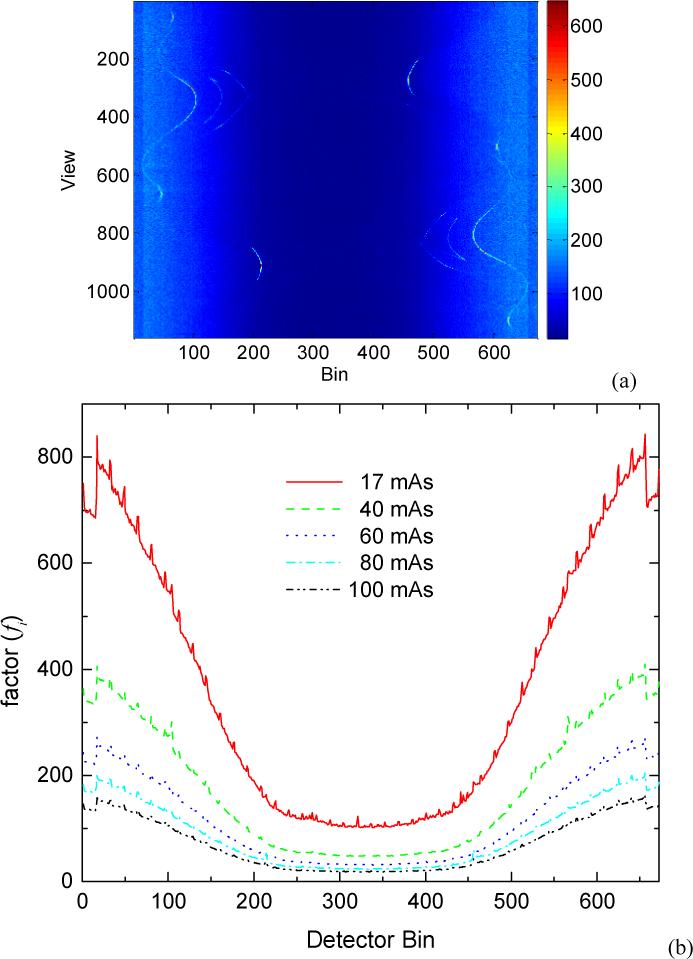
Factor f_i in equation (7) calculated from 150 repeated measurements at 100 mAs level for all data channels, i.e., 672 detector bins and 1160 views (a). Each curve represents an average over the 1160 views at a corresponding mAs level (b).

The similarity of {f_i} curves for different mAs values was further studied by plotting the paired points (f_i,100, f_i,mAs), where f_i,100 is the f_i value at the 100 mAs level while f_i,mAs is the value at a lower mAs level. Figure 3 shows the plots of the paired points. A linear relationship can be observed for each of the four mAs levels. The slopes of these four lines were determined by linear fitting and their values are shown by the four points at 17, 40, 60, 80 mAs in Figure 4. Essentially, all these four slope values are closely represented by the corresponding ratios of f_i,mAs / f_i,100 . The relationship between the ratios of f_i,mAs / f_i,100 and the mAs values can be described by a reciprocal function:

$$y=1∕(a+bx)$$ (9)

as shown in Figure 4. Ideally, the ratios of f_i,mAs / f_i,100 would be inversely and linearly proportional to the ratio of the corresponding mAs values (see equation (6)), i.e., the parameter a in equation (9) would be zero. The obtained parameter a indeed is relatively small as compared to b times mAs level (or the x value). A major reason for a non-zero a value is due to the electronic background noise which plays a noticeable role when the mAs value is small, i.e., the fitted curve in Figure 4 deviates from a straight line as mAs value becomes smaller. An additional possible reason for the presence of non-zero a could be that the mAs values reported by the CT scanner consol did not reflect the actual tube current, causing the nonlinearity of the variance versus the reported mAs values. The likelihood of this additional possible reason is very low because the clinical scanner is under quality control for daily patient operation.

Figure 3.

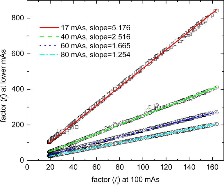
Illustration of a linear relationship between f_i value at 100 mAs level and f_i values at other lower mAs levels.

Figure 4.

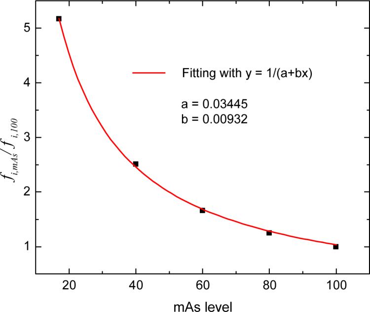
Factors of f_i,mAs / f_i,100 at five different mAs levels and their fitted curve with a reciprocal functional. Given this curve and the shape of f_i in Figure 2, the variance at any mAs level can be estimated.

The similarity of {f_i} curves for different attenuating conditions (i.e., 1160 view angles around the anthropomorphic torso phantom) and different mAs values for each view angle indicates that parameter f_i is object-independent, concurring with the theoretical analysis in Section II. Its global shape reflects the bowtie filtration and its local variation indicates the detector bin response. Given the shape of {f_i} in Figure 2 and the curve of f_i,mAs / f_i,100 in Figure 4, we are able to estimate the variance of the sinogram at any mAs level by the theoretical model (7) for practical purposes.

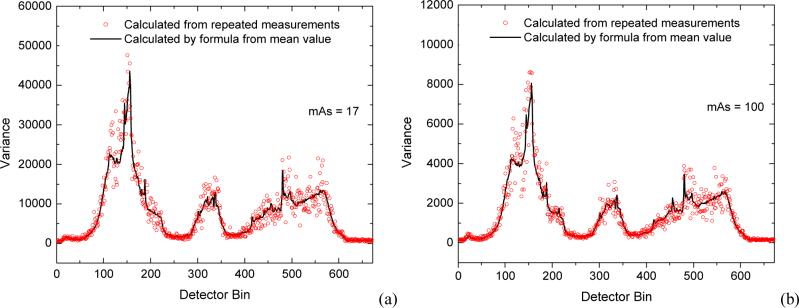
To further validate the above noise model (7) across the FOV, we compared the experimental sample variances calculated from the repeated scans with the theoretical variances predicted by equation (7) for each of the 1160 views. An example is presented below for an arbitrarily selected projection view. For each mAs level, the experimental sample variances for that view have been calculated previously when we computed the pairs (p̃_i, ${\sigma }_{p_i}^2$) for each detector bin i for a total of 672 bins. The theoretical variances were determined as follows. Given the sample mean p̃_i at that view and the above determined parameter f_i from all 1160 views and η =2294.5 for the CT system, the corresponding theoretical variance ${\sigma }_{p_i}^2$ can be computed by (7). Good consistency between the experimental sample variances and the theoretically predicted variances was observed for all mAs values. Figure 5 shows two comparisons at 17 and 100 mAs levels for the selected view. To quantitatively measure the consistency between the variance predicted by (7) and the experimental sample variance calculated from the repeated scans, we computed the Lin's concordance correlation coefficients (Lin 1989) at all mAs values. The results are shown in Table I. It can be observed that all of Lin's concordance coefficients are larger than 0.9, even in the cases where all lower bounds of the 95% confidence interval of the correlation coefficients are larger than 0.9, suggesting an excellent agreement between experimental and predicted variances. This agreement was also visually seen from repeated measurements of a different commercial (GE HiSpeed four-slice) CT scanner as reported in the work of Li et al 2004.

Figure 5.

Illustration of sinogram data variances calculated from repeated scans and from equation (7). (a)–result at 17 mAs, and (b)–result at 100 mAs. These variances from the repeated scans and from the prediction of equation (7) agree with each other very well.

Table I.

Lin's concordance correlation coefficient between experimental and theoretical variances at different mAs levels.

mAs level	Sample Size N	Lin's Concordance Coefficient	95% Confidence Interval of Concordance Coefficient
100	672	0.958	(0.952, 0.964)
80	672	0.961	(0.954, 0.966)
60	672	0.913	(0.900, 0.925)
40	672	0.941	(0.932, 0.949)
17	672	0.953	(0.945, 0.959)

In the following, we turn our attention to the normality test of the repeatedly measured samples for each channel. The statistical normality test was performed for all detector bins (i.e., 672) over all projection views (i.e., 1160), or a total of 672×1160 channels with each channel consisting of 150 random samples. The Shapiro-Wilk normality test was employed via the use of the program R, which is a free software environment for statistical analysis and can be downloaded at (http://www.r-project.org/index.html).

The null hypothesis H₀ in the normality test is stated as follows. The acquired 150 data values from each channel are random samples from a normal distribution. If the probability (p-value) is less than the level of significance (e.g., 0.05 for 95% level was chosen in this study), then the null hypothesis is rejected. The Shapiro-Wilk test gives the p-value for each of the 150 repeated measurements at each channel. A smaller p-value indicates that the projection data at that channel is less likely to follow a normal distribution. The rejection percentage (those channels whose p-values are less than 0.05 divided by the total number of channels in each sinogram) for each mAs value is shown in Figure 6. It can be observed that the rejection percentages increased from approximately 6% at 100 mAs level up to 9% at 17 mAs level for all data channels.

Figure 6.

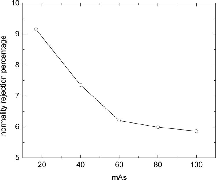
Rejection percentage of the Shapiro-Wilk normality test for sinogram data at different mAs levels.

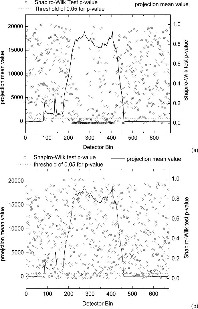
To view the p-value distribution across the FOV, we plotted Figure 7, which shows the relationship between projection mean value and Shapiro-Wilk test p-value at different detector bins at a projection view. Figure 7(a) shows the result from the 17 mAs value and Figure 7(b) represents the result from the 100 mAs value. Compare the Shapiro-Wilk test p-values at the 17 mAs level with that at the 100 mAs level for the same projection view, we can observe that small p-values less than 0.05 occur mostly at those detector bins where the X-rays pass through the most dense parts of the body, corresponding to the high projection mean values or low-flux transmitted data. As the mAs value decreases, less X-ray photons will be generated and detected and, therefore, less projection data will pass the Shapiro-Wilk normality test.

Figure 7.

Relationship between projection mean value and the Shapiro-Wilk test p-value at different detector bins by the same projection view for 17 mAs level (a) and 100 mAs level (b).

Based on Figure 7, we further computed the rejection percentage at the low flux region. For those high projection-mean values greater than 10000, the rejection percentage increased from 7.03% at 100 mAs level to 18.40% at 17 mAs level. The rejection percentage increased at a higher speed for a larger projection-mean value. For example, the rejection percentage increased from 9.95% at 100 mAs level to 41.95% at 17 mAs for projection mean values greater than 15000.

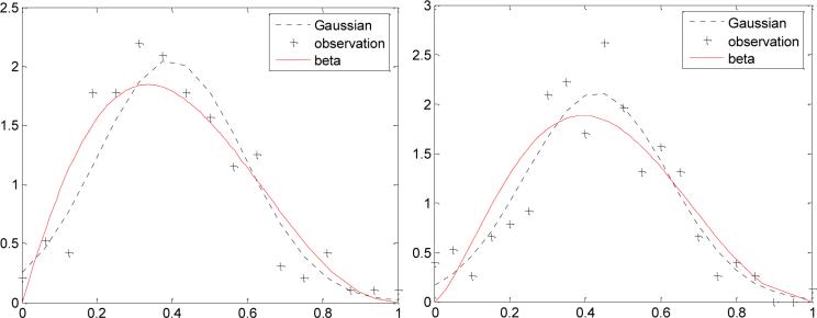
For those detector bins with p-values less than 0.05 at the 17 mAs level in Figure 7, we further studied their noise distribution in terms of probability density function (PDF). Figure 8 shows, as an example, the PDF from detector bin #120 (left) and detector bin #376 (right) at the 17 mAs level in Figure 7. Their corresponding p-values from the Shapiro-Wilk normality test are less than 0.001. It can be observed that for a very small p-value (i.e., a highly likely non-normal distribution), the PDF did reveal some deviation from a Gaussian or normal distribution. The deviation from a normal distribution can be quantitatively measured by higher statistical moments, such as skewness and kurtosis. Table II lists the statistical moments for several detector bins with high mean values at the 17 mAs level and small p-values (<0.05) from the Shapiro-Wilk normality test. It can be observed that for those detector bins with small p-value (<0.05) from the Shapiro-Wilk normality test, their corresponding skewness or kurtosis are generally non-zero (both skewness and kurtosis would be zero for Gaussian distribution). It is noted that despite the deviation from a normal distribution as seen in Figure 8, the measured PDF fits Gaussian better than Poisson, Gamma and Beta functional forms because all of these latter distributions do not have the mean-variance relationship of (7). The fitting to the Beta distribution is shown in Figure 8 as an example. Since both the Gamma and Beta functions are much more complicated in numerical calculation than the Poisson and Gaussian forms, there is no significant benefit to consider the Gamma and Beta PDFs in Radon space. Since the Poisson distribution does not satisfy the mean-variance relationship of (7), it cannot be a better choice than the Gaussian if an approximated PDF is needed.

Figure 8.

Probability density function from detector bin #120 (left) and #376 (right) at 17 mAs level. Its corresponding p-value from the Shapiro-Wilk test is 0.001. The dotted line represents a fitting to a Gaussian distribution. The solid line shows a fitting to a Beta function.

Table II.

Statistics for the detector bins with high mean value.

Detector Bin	Mean Value	Normality Test p-value	Skewness	Kurtosis
376	16118	0.00103	−0.09708	−0.67877
377	15994	7.890E-7	0.32897	0.73426
378	15918	0.17249	0.20178	0.48699
379	16027	0.03228	−0.16628	0.11167
380	16171	0.04202	0.12740	−0.28743
381	16281	0.61378	0.13290	−0.00143
382	16428	0.00134	0.11541	0.29458
383	16595	0.16667	0.23176	0.02940
384	16758	0.09693	−0.03816	−0.05951
385	16837	0.14875	0.17857	−0.14606

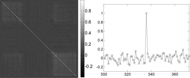
In addition to the studies on the mean-variance relationship and the normality tests of noise distribution in the sinogram, we also analyzed the noise correlation among different bins. Figure 9(a) displays the correlation coefficients matrix of the noise among detector bins at one view from the repeated measurements of the Siemens scanner at the 17 mAs level. Figure 9(b) shows the horizontal profiles through the center of Figure 9(a). The average of the off-diagonal values from Figure 9(a) was calculated as 0.0042. It can be seen that only the diagonal value is equal to 1 while the off-diagonal values are close to zero, indicating that the noise is independent from each other among the detector bins. This result is consistent with the noise correlation analysis from repeated measurements of a different commercial (GE HiSpeed four-slice) CT scanner as reported in the work of Wang et al 2006a. The noise independence is important to specify the likelihood function for a penalized maximum likelihood approach.

Figure 9.

Correlation coefficients matrix of noise among detector bins from repeated measurements of a view angle at 17 mAs level (left). On the right is the horizontal profile through the center of the picture on the left. It can be observed that only the diagonal value is equal to 1 while the off-diagonal values are close to zero.

IV. Discussions

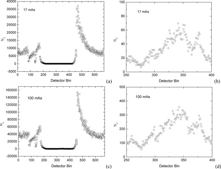
The mean-variance relationship of formula (7) is theoretically based on equations (3) and (4). One assumption during the derivation of equations (3) and (4) is that the chance of detecting zero photon number is small because of the logarithm transform. Given the line integral variance ${\sigma }_{p_i}^2$ from the repeated measurements, the mean of the transmitted photon number N_d can be estimated according to equation (4). The range of the transmitted photon number varies noticeably at different bins and also at different mAs levels. Figure 10 shows the number of transmitted photons at the same projection view as in Figure 7. It can be observed that even at the 17 mAs level, the minimum number of transmitted photons is approximately 10. The probability of receiving a zero photon number for a random variable of Poisson distribution with mean value 10 is very small (4.5×10⁻⁵). Therefore, the assumption behind the equations (3) and (4) generally holds in all the experiments reported in this paper up to the lowest level of 17 mAs.

Figure 10.

Number of transmitted photons along one projection view at (a)– 17 mAs level and (c)– 100 mAs level for all detector bins. Pictures (b) and (d) show the details for those detector bins between 250 and 400 for the 17 mAs and the 100 mAs levels respectively.

As shown in Figure 7, a significant quantity of sinogram data from the highly attenuating region at very low mAs level (17 mAs) failed the normality test (i.e., their p-values are less than 0.05). Strictly speaking, their PDFs can not be expressed as a Gaussian normal functional. Therefore, a cost function of the Gaussian functional for noise reduction and image reconstruction at such low mAs levels may not be mathematically adequate, despite it is a better choice compared to others, such as Poisson, Gamma, etc.

Theoretically, the compound Poisson PDF would be an option to construct a cost function for statistical noise treatment and image reconstruction from the transmitted projection data in the transmission space (Snyder et al 1991, Whiting et al 2006). In the transmission space, image reconstruction from the transmitted data is a nonlinear problem because the system matrix relating the source to the data is nonlinear, i.e., N_d = N₀ exp(−∫μ ds). It is well-known that solving a nonlinear problem is much more challenging than solving a linear problem of p = ∫μ ds . The solution of a non-linear system is less stable than that of a linear system in the presence of noise. In addition, minimizing the compound Poisson cost function is numerically tedious and, therefore, an approximation by the Poisson distribution is usually taken. If the Poisson distribution is taken, equations (3) and (4) hold and, therefore, the mean-variance relationship of formula (7) may reflect the transmitted-data noise properties in Radon space.

Seeking an adequate PDF for the sinogram data in Radon space, where image reconstruction from the sinogram data is a linear problem (i.e., p = ∫μ ds), remains an active research topic (Lu et al 2001, 2002, Li et al 2004). If the exact PDF is unknown but close to a normal distribution, as shown in Figure 8, a penalized weighted least-squares (PWLS) cost function could be an optimal choice, which fully utilizes the relationship between the first and second statistical moments. Our previous work utilizing this alternative approach has generated very encouraging results in terms of high computational efficiency and reconstruction accuracy as measured by noise-resolution tradeoff and receiver operating characteristic (ROC) merits (Wang et al 2006a and 2006b).

It is noted that the mean-variance relationship (7) was based on the first-order Taylor expansion and did not include explicitly the electronic background noise, although the presence of the electronic background noise in the experimental data was considered implicitly by fitting the adaptive factor f_i and could be seen in Figure 4. The relationship (7) mainly considers the bowtie filtration effect which causes the data variance variation by more than five folds across the FOV (see Figure 2). By considering this effect, the PWLS approach has shown a significant gain for low mAs (or low-dose) CT imaging. This gain reveals that it is worth to spend more effort to include explicitly the electronic background noise and possibly higher order Taylor expansions for further dose reduction in CT imaging.

V. Conclusion

In this work, we studied the noise properties of CT sinogram data at low mAs levels through repeated experiments on an anthropomorphic torso phantom. We performed the Shapiro-Wilk normality test on the repeated measurements and found that data channels at highly attenuating regions failed the test at very low mAs levels.

Based on the repeated experiments, we validated the mean-variance relationship of (7) for each data channel at different mAs levels. This relationship reflects that the major noise factor is due to the Poisson distribution of the transmitted photons and the bowtie attenuating filtration. The variance of projection data at a specific detector bin are completely determined by two physical quantities: (1) the line integral (i.e., p̃_i) of attenuation coefficients along the X-ray path and (2) the incident photon number (i.e., N_0i). Our noise model of equation (7) considered these two quantities elegantly. The first quantity is reflected by p̃_i /η in equation (7), where η is a system-specific scaling parameter. The second quantity is reflected by f_i in equation (7). From our systematic studies using the repeated measurements, it can be observed that factor f_i primarily depends on the incident photon number (or the mAs value) and the shape of the bowtie attenuating filter across the FOV. Essentially, f_i is determined by the incident photon number at each specified detector bin. The validated non-linear mean-variance relationship of (7) precludes the use of Poisson, Gamma or other PDF, which has a different mean-variance relationship, as a cost function for noise reduction and image reconstruction in Radon space.

Given equation (7) and Figure 2, we are able to predict the sinogram variances very accurately from the corresponding projection data acquired at a mAs value. In other words, equation (7) reflects the ground truth for the weights of the WLS criterion, while the noise independence among detector bins (see Figure 9) supports the LS criterion. By further considering the spatial correlation of sinogram data among nearby channels or image density distribution among nearby voxels, the PWLS cost function for sinogram restoration or image reconstruction would be a choice for low-mAs CT imaging. It is expected that the gained knowledge on the noise properties of the low-mAs sinogram data in this experimental work would assist the sophisticated image reconstruction methodologies in current CT scanners to address the noise problem in low-dose CT clinical applications.

Our previous research effort (Wang et al 2006a and 2006b) has shown that the PWLS cost function has a great potential for use in low-mAs CT imaging. This experimental work provides both a ground truth for the use of the PWLS cost function and an encouragement for further investigation on the mean-variance relationship by considering higher order effects (such as the electronic background noise) and refining the PWLS optimization strategy.

References

- Herman GT. “Image Reconstruction from Projections”. Academic Press; New York: 1980. [Google Scholar]
- Li T, Li X, Wang J, Wen J, Lu H, Hsieh J, Liang Z. “Nonlinear sinogram smoothing for low-dose X-ray CT”. IEEE Trans. Nuclear Science. 2004;51(4):2505–2513. [Google Scholar]
- Lin LIK. “A concordance correlation coefficients to evaluate reproducibility”. Biometrics. 1989;45(3):255–268. [PubMed] [Google Scholar]
- Linton OW, Mettler FA. “National conference on dose reduction in CT, with an emphasis on pediatric patients”. American Journal of Roentgenology. 2003;181(2):321–329. doi: 10.2214/ajr.181.2.1810321. [DOI] [PubMed] [Google Scholar]
- Lu H, Hsiao I-T, Li X, Liang Z. “Noise properties of low-dose CT projections and noise treatment by scale transformations”. Conference record of IEEE NSS and MIC; San Diego, CA, USA. Nov. 4−10, 2001.2001. pp. 1662–1666. [Google Scholar]
- Lu H, Li X, Hsiao I-T, Liang Z. “Analytical noise treatment for low-dose CT projection data by penalized weighted least-square smoothing in the K-L domain”. SPIE Medical Imaging; San Diego, CA, USA. Feb. 23−28, 2002.2002. pp. 146–152. [Google Scholar]
- Macovski A. “Medical Imaging Systems”. Prentice-Hall Inc; New York: 1982. [Google Scholar]
- Snyder DL, Miller ML. “Random point Processes in Time and Space”. Springer-Vertag; New York: 1991. [Google Scholar]
- Wang J, Li T, Lu H, Liang Z. “Penalized weighted least-squares approach to sinogram noise reduction and image reconstruction for low-dose X-ray computed tomography. IEEE Trans. Medical Imaging. 2006a;25(10):1272–1283. doi: 10.1109/42.896783. [DOI] [PMC free article] [PubMed] [Google Scholar]
- Wang J, Li T, Lu H, Liang Z. “Noise reduction for low-dose single-slice helical CT sinograms”. IEEE Trans. Nuclear Science. 2006b;53(3):1230–1237. doi: 10.1109/tns.2006.874955. [DOI] [PMC free article] [PubMed] [Google Scholar]
- Whiting BR, Massoumzadeh P, Earl OA, O'Sullivan JA, Snyder DL, Williamson JF. “Properties of preprocessed sinogram data in X-ray computed tomography”. Medical Physics. 2006;33(9):3290–3302. doi: 10.1118/1.2230762. [DOI] [PubMed] [Google Scholar]