Mixed Effects Models for Quantitative Trait Loci Mapping With Inbred Strains

Abstract

Fixed effects models have dominated the statistical analysis of genetic crosses between inbred strains. In spite of their popularity, the traditional models ignore polygenic background and must be tailored to each specific cross. We reexamine the role of random effect models in gene mapping with inbred strains. The biggest difficulty in implementing random effect models is the lack of a coherent way of calculating trait covariances between relatives. The standard model for outbred populations is based on premises of genetic equilibrium that simply do not apply to crosses between inbred strains since every animal in a strain is genetically identical and completely homozygous. We fill this theoretical gap by introducing novel combinatorial entities called strain coefficients. With an appropriate theory, it is possible to reformulate QTL mapping and QTL association analysis as an application of mixed models involving both fixed and random effects. After developing this theory, our first example compares the mixed effects model to a standard fixed effects model using simulated advanced intercross line (AIL) data. Our second example deals with hormone data. Here multivariate traits and parameter identifiability questions arise. Our final example involves random mating among eight strains and vividly demonstrates the versatility of our models.

IN analyzing gene mapping data from inbred strains, there is always the temptation to borrow models more pertinent to outbred populations. The vast majority of statisticians are wise enough to resist this temptation and turn to analysis methods tailored to specific breeding designs. Fortunately, the typical backcross or F₂ design has sufficient symmetry to permit analysis of variance by standard statistical packages. As mammalian geneticists explore more complicated designs involving multiple strains and multiple generations, this analysis paradigm has begun to fracture. It is therefore hardly surprising that the last decade and a half have seen a revival of interest in statistical models for gene mapping with inbred strains. Although we briefly review some of the important contributions to this literature in the next section, it is fair to say that most modern models rely heavily on fixed effects. In contrast, the most successful models for mapping quantitative trait loci (QTL) in outbred populations invoke random effects (Hopper and Mathews 1982; Goldgar 1990; Schork 1993; Amos 1994; Blangero and Almasy 1997).

The premise of this article is that, properly formulated, random effects models hold equal promise for more complicated inbred strain data. If a QTL is segregating between two strains, backcross and F₂ designs reliably detect it (Valdar et al. 2006). Models based on fixed allelic effects play a critical role in this process. Traditional designs have two drawbacks. First, the scarcity of recombination events often gives long mapped intervals. Second, when two founder strains of related ancestry are chosen, there may be no segregating QTL. To increase the number of recombination events and the number of segregating QTL, geneticists are turning to more complex designs involving multiple strains. Although the rationale for more complex designs is compelling, they bring in their wake problems of overparameterization. Random effects models neatly circumvent some of the parameterization issues encountered with fixed effects models. Unfortunately, the standard outbred QTL model does not make sense for inbred strains. All individuals of a particular strain are genetically identical and completely homozygous. These cardinal characteristics have subtle consequences when we calculate trait covariances for the descendants of matings between different strains. A logically correct theory for specifying covariances between pairs of individuals is the key to making random effects models respectable for inbred strains.

In this article, we take two approaches to QTL mapping; both capture polygenic background as a source of random variation. The two approaches differ in how they handle variation caused by the QTL. In association mapping, markers are treated one by one as candidate genes, and observed genotypes or allele counts at a marker serve as fixed predictors of trait means. In linkage mapping, markers in the vicinity of the QTL provide prior information on gene sharing, and the QTL contribution is modeled as a random effect. The greatest defect of our models is the blanket assumption of additivity. The greatest strength of our models is their generality in other regards. Thus, there is no limit to the number of founding strains, the depth and complexity of pedigrees, or the number of traits in a multivariate analysis.

To avoid breaking the flow of our discussion, much of the mathematical detail is relegated to the appendixes. The following sections summarize previous contributions, lay out the model with full attention to computation of strain coefficients and relative covariances, resolve the thorny issue of identifiability, apply the models to real and simulated data, and discuss the broader implications and limitations of the models.

METHODS

A brief survey of previous methods:

Inbred mammalian strains have unique advantages in genetics. All members of a strain are genetically identical and completely homozygous. Simple crosses between strains involve no phase ambiguities, and any genes mapped can be quickly located in humans and other species by synteny. With mice and other small mammals, breeding is reasonably straightforward, generation times are fairly short, and the environment can be exquisitely controlled.

For decades, QTL mapping in inbred strains was considered an exercise in fixed effects modeling. Testing for association between marker genotypes and trait values is readily carried out using several available statistical packages. In the interval method introduced by Lander and Botstein (1989), the QTL is allowed to take any position along a chromosome. This makes QTL genotypes unobservable and requires computation of posterior distributions given observed genotypes at the flanking markers. Although the EM algorithm is applicable in this context, it is often slow to converge, and the regression method of Haley and Knott (1992) provides a quick approximation. The permutation test of Churchill and Doerge (1994) handles multiple testing problems gracefully. The recent program R/qtl (Broman et al. 2003), which capitalizes on the R software environment, combines several of these methods with hidden Markov modeling of missing genotypes. Despite these admirable advances, interval mapping is still limited to simple crosses where polygenic background is confounded with random environment. As the field embraces more complex crosses, geneticists no longer have the luxury of ignoring polygenic background, and it seems self-evident that explicitly modeling it will improve statistical inference.

The composite interval mapping method of Zeng (1993, 1994) implemented in QTL Cartographer generalizes interval mapping by including the direct effects of one or more markers unlinked to the QTL. Hence, composite interval mapping can be viewed as an attempt to incorporate polygenic background through fixed effects. If the number of typed markers is large, then it becomes hopeless to include all of them, and some automatic selection of background markers is desirable (Manly and Olson 1999).

Although Xie et al. (1989) take important first steps toward including polygenic background as a random effect, they do not derive general covariance expressions. This failure makes it difficult to deal with nonstandard crosses and awkward to combine data from different crosses. In the meantime, the pressure to increase the number of strains per cross has been growing (Rebai and Goffinet 1993). Of 21 cloned mouse genes listed in Tables 1 and 2 of the review by Flint et al. (2005), 7 rely on cloning strategies involving multiple strains or outbred mice. These practical concerns are stimulating intense efforts to revamp experimental design and statistical analysis of inbred cross data (Liu and Zeng 2000; Hitzemann et al. 2002; Pletcher et al. 2004; Li et al. 2005; Cervino et al. 2007). Other recent models that delve into multiple QTL models and epistasis are both frequentist (Kao et al. 1999; Janninka and Jansena 2001; Seaton et al. 2002; Broman et al. 2003) and Bayesian oriented (Sillanpää and Arjas 1998; Sen and Churchill 2001; Broman et al. 2003).

TABLE 1.

AIL: type I error, power, coverage, and average estimates

	Mendel Full	Mendel F10	Cartographer	True value
Type I error	0.83–3.39	4.92–9.60	25.6–33.8	NA
Power	96	46	51	NA
Coverage	92	39	48	NA
Point 5
η	3.9913 (0.2058)	3.9661 (0.2355)	NA	4.000
p1	0.6486 (0.1183)	0.3259 (0.0878)	NA	0.667
ɛ1	0.1910 (0.0487)	0.1759 (0.0764)	0.1869	0.200
ɛ2	−0.1910 (0.0487)	−0.1759 (0.0764)	−0.1869	−0.200
	1.0112 (0.1002)	1.1494 (0.1721)	0.9581	1.000
Point 6
η	3.9998 (0.2059)	3.9465 (0.2344)	NA	4.000
p1	0.6492 (0.1176)	0.3370 (0.0967)	NA	0.667
ɛ1	0.1932 (0.0477)	0.1764 (0.0758)	0.1781	0.200
ɛ2	−0.1932 (0.0477)	−0.1764 (0.0758)	−0.1781	−0.200
	1.0092 (0.0998)	1.1458 (0.1746)	0.9606	1.000

Type I error rates, power, and coverage are percentages; estimates and standard errors are averages. Type I error rates are confidence intervals based on 500 simulations under the null hypothesis; other table entries are based on 100 simulations under the alternative hypothesis. We count successful coverage when the equivalent one-LOD drop (4.6 LRT units) interval around a significant map point includes the QTL. The QTL is located at the midpoint of points 5 and 6. Parameter p₁ is the reduced-dimension polygenic background parameter; η, the grand mean; ɛ_i, the QTL effect on strain i; and , the residual covariance. The Mendel estimates have average standard errors in parentheses. NA, not applicable.

TABLE 2.

Four-way cross: mean estimates for bivariate leptin analysis at D3Mit127

	Lep-4		Lep-15
Mean effect	Estimate	SE	Estimate	SE
B6/C3	0.1273	0.0616	0.1258	0.0638
B6/D2	−0.1686	0.0599	−0.1675	0.0632
C/C3	0.1812	0.0593	0.1198	0.0615
C/D2	−0.1399	0.0615	−0.0781	0.0646
Grand	−0.0157	0.0346	−0.0243	0.0362

SE, standard error.

Trait means, variances, and covariances:

We begin our theory development with a basic model applicable to any inbred strain design, including F₂, advanced intercross lines, and random mating. Suppose that i and j are two animals generated by a complex cross involving s inbred strains. At t traits of interest, i and j exhibit random vectors X_i and X_j of trait values. For the sake of simplicity, assume further that X_i and X_j reflect the contributions of a single gene whose alleles have additive effects. Our immediate goal is to calculate the expected vectors E(X_i) and E(X_j) and the covariance matrix Cov(X_i, X_j). When i = j, we recover variances as well as covariances. Because of our assumption of additivity, X_i decomposes as the sum Y_i + Z_i of a maternal contribution Y_i plus a paternal contribution Z_i. To calculate E(Y_i), let M_i denote the originating strain of the maternal gene of i. Although M_i is unobserved, we can calculate the probability Pr(M_i = a) for any given strain a. In terms of these probabilities and the t × 1 mean vector μ(a) of allelic effects on each trait for strain a, we have

Invoking a similar expression for E(Z_i), it follows that

(1)

where γ_i(a) is the probability that a randomly sampled gene from i originates from strain a. We refer to γ_i as the strain fraction vector for animal i; γ_i has dimension s × 1.

Covariances are derived by the same kind of reasoning. Decompose X_j into the sum V_j + W_j of a maternal contribution V_j plus a paternal contribution W_j. In view of the bilinearity of the covariance operator and the symmetry of maternal and paternal alleles, it suffices to find the covariance Cov(Y_i, V_j). Let N_j denote the originating strain of the maternal gene of j. Conditioning on the joint value of M_i and N_j then yields

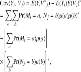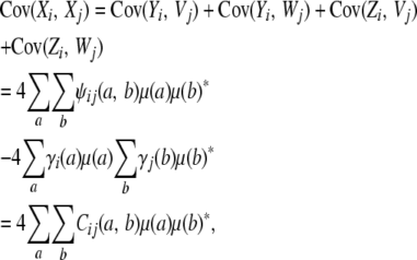
where the superscript * indicates a vector or matrix transpose. By analogy with kinship coefficients, we define the strain coefficient ψ_ij(a, b) to be the joint probability that a randomly drawn gene from animal i originates from strain a and a randomly drawn gene from the same locus of animal j originates from strain b. If i and j coincide, then sampling is done with replacement. The t × t covariance matrix between the trait values of i and j becomes

(2)

where C_ij(a, b) = ψ_ij(a, b) − γ_i(a)γ_j(b), which we collect into an s × s matrix, denoted C_ij.

For s strains and t traits, it is convenient to stack the allelic effects into a column vector μ of length st with transpose

The positive semidefinite matrix Ω = μμ* can then be split into t² blocks Ω_kl each of size s × s. Restricting our attention to the block corresponding to traits k and l, the covariance matrix (2) has entries given by the trace formula

(3)

In polygenic inheritance, many independent loci contribute in an additive manner to the traits under consideration. Since trait means and covariances add in this setting, the mean expression (1) and the covariance expressions (2) and (3) remain valid provided we replace μ by and Ω by . Here μ^l denotes the vector contribution corresponding to locus l rather than the lth component of μ. appendix a shows that every pair (μ, Ω) consisting of a vector μ and a positive semidefinite matrix Ω can be represented as two such coordinated linear combinations. Hence, to capture polygenic background, it suffices to estimate arbitrary μ and Ω. We see later that there is an identifiability issue that must be surmounted in estimating Ω.

Computation of strain coefficients:

Because the combinatorial coefficients γ_i(a) and ψ_ij(a, b) are essential in calculating trait means and variances, we need good algorithms to compute these coefficients. Fortunately, we can mimic the logic used in calculating kinship coefficients for outbred populations. Since a pedigree founder i is assumed to be strain pure, one entry of the vector γ_i = 1, and the remaining entries = 0. Likewise for two founders i and j, one entry of the matrix ψ_ij = 1, and the remaining entries = 0. All other strain fraction vectors γ_i and strain coefficient matrices ψ_ij are defined recursively starting with the founders.

To avoid circular reasoning, pedigree members are numbered so that parents always precede their children. If animal i is not a founder, then it has parents k and l. Assuming that k and l have already been visited in filling in the strain fractions, we set

(4)

If j ≠ i, then without loss of generality we can assume j has been visited already, and we can set

(5)

(6)

This leaves only the case j = i. There are four equally likely possibilities when we sample two genes of i: (a) both genes coincide with the gene passed by k, (b) both genes coincide with the gene passed by l, (c) the first gene comes from k and the second from l, and (d) the first gene comes from l and the second from k. These considerations produce the matrix recurrence

(7)

where diag(γ) denotes a diagonal matrix whose diagonal entries coincide with the entries of the vector γ.

The initial conditions on founders and the recurrences (4)–(7) completely determine γ_i and ψ_ij. These in turn determine the C_ij matrices, which have a richer mathematical structure than the strain coefficient matrices ψ_ij. appendix b describes several fascinating properties of the C_ij matrices. One such property is C_ij = 0 between most members of simple crosses, for example, for all F₂ animals when i ≠ j or whenever i is a founder or F₁.

Variance component models for QTL mapping with outbred populations require conditional kinship coefficients in addition to theoretical kinship coefficients. For exactly the same reasons, we also need conditional strain fractions and coefficient matrices. These depend on observed marker genotypes in the vicinity of a putative QTL. On small pedigrees, it is possible to compute conditional strain coefficient matrices exactly by considering all descent graphs (gene flow patterns) at the QTL and neighboring markers (Kruglyak et al. 1996). In practice, inbred strain pedigrees are so large that the number of possible descent graphs is astronomical. Stochastic sampling provides a workable substitute for exhaustive enumeration of descent graphs (Sobel and Lange 1996). The Markov chain Monte Carlo (MCMC) method incorporated in the computer program SimWalk samples relevant descent graphs with the appropriate conditional probabilities. Given a descent graph at the QTL, it is trivial to compute strain fractions for all animals and strain coefficient matrices for all pairs of animals in a pedigree. The averages of these quantities over all sampled descent graphs serve as approximations to the conditional strain fractions and strain coefficient matrices.

Strain coefficients convey more information than strain fractions. For instance, it is obvious that

We can put this extra information to good use in predicting QTL genotypes. At a given genomic location, imagine a marker with a different allele for each strain. Let be the conditional probability that animal i has unordered genotype a/b at the hypothetical marker given the observed data at the ordinary markers. The relations

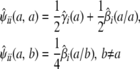connect the conditional genotype probabilities to the conditional strain fractions and coefficients. These relations in turn imply that

(8)

Thus, we can impute strain genotypes as well as strain fractions.

Variance component models:

Variance component models revolve around the multivariate normal distribution or related distributions such as the multivariate t. Every multivariate normal distribution is uniquely determined by its mean vector ν and variance matrix Σ. If we decompose trait values into independent, additive contributions, then ν and Σ can be expressed as sums over the various contributions. As long as we are willing to take the leap of faith that all random contributions are Gaussian, then trait vectors will be Gaussian as well. For each random contribution, variance matrices are constructed from a constant part and a parametric part. The genetic covariance formula (3) is typical in this regard. The constant parts C_ij are forced on us by the nature of the pedigree. The parametric part Ω with blocks Ω_kl requires estimation.

The environmental contribution to the mean is usually modeled as the sum of a grand mean η plus covariate effects such as age or sex. Random environment and cage effects can be modeled by Kronecker products of variance matrices, provided we order trait values so that all values corresponding to a given trait are contained in a single block, and animals are consistently enumerated across blocks. Given these conventions, the variance matrix under random environment reduces to the Kronecker product ϒ ⊗ I of the trait variance matrix ϒ and the identity matrix I. Obviously, ϒ is the parametric part; it describes the environmental covariation of the traits in a single animal. The matrix I reflects the independence of the random environments for the various animals. For a random cage effect, we replace the identity matrix by a cage matrix H = (h_ij), where h_ij = 1 if animals i and j belong to the same cage and 0 otherwise. The matrix replacing ϒ describes the environmental covariation of the traits for animals in a single cage (Lange 2002). As an example, heritability analyses generally specify two random effects, additive polygenes and random error/environment,

(9)

(10)

where α_ic is the cth of C covariates measured on animal i and β_kc is the corresponding regression coefficient for trait k.

Once we specify the mean and variance components, the loglikelihood of a pedigree can be written as

using the observed trait values x, the mean vector ν such as that of Equation 9, and the variance matrix Σ such as that of Equation 10. Assuming pedigrees behave independently, their loglikelihoods add. Given the overall loglikelihood, parameters can be estimated by maximum likelihood, and statistical inference conducted by standard likelihood ratio tests comparing alternative hypotheses to null hypotheses. Lange (2002) develops this frequentist approach to estimation and inference in detail. Our computer program Mendel relies on a quasi-Newton algorithm for maximum likelihood estimation. Bauman et al. (2005) discusses an alternative EM algorithm as well as factor-analytic parameterizations of variance matrices. Given the presence of covariates and heterogenous pedigree structures, permutation testing is rarely possible. To aid the user in judging significance and model fitting, Mendel reports standard errors of parameters, pedigree deviances, outlier individuals, and various goodness-of-fit statistics.

Two QTL mapping strategies:

There are two specific strategies, association and linkage, for QTL mapping. Variance component models are pertinent to both. Although the two strategies differ in how they portray QTL effects, each captures polygenic background as a random effect. In addition to the strain effects appearing in Equation 1, most models include a grand mean η and fixed effects tied to plausible predictors. If we specify η, then we must impose the vector constraint on the polygenic mean vector μ. Here the index a ranges over all strains. Random effects include the polygenic effect summarized by Equation 3, random environment plus measurement error, and possibly correlated environment such as cage effects. As described in the next section, the polygenic variance matrix Ω is not identifiable, and complicated constraints must be imposed on it to compensate for this fact. Regardless of the nature of these constraints, we must compute theoretical strain fractions and strain coefficients to estimate μ and Ω under the null hypothesis of no QTL effect.

In linkage mapping, markers serve to tag chromosome segments and keep track of recombination events. The genotypes of the causative QTL are unobserved, and the QTL is allowed to assume any position along the genome. Under the alternative hypothesis in linkage mapping, we model the QTL as a random effect in the same way that we modeled the contribution of a single gene with additive effects. The only difference is that we use strain fractions and coefficients calculated conditional on the observed marker data. From here on, we refer to these as conditional strain fractions and coefficients; those calculated unconditionally we call theoretical strain fractions and coefficients. Motivated by Equations 1 and 3, we let ɛ(a) denote the additive effect of the QTL in strain a. Then our earlier reasoning shows that the QTL contribution has mean

for animal i and covariance

for animals i and j. Here the circumflexes indicate conditional versions of the strain fractions and coefficients estimated from the marker data. Under the alternative hypothesis, we estimate the entries of ɛ.

Our basic linkage model therefore specifies the trait means and covariances

(11)

(12)

for two animals i and j. Here k and l index two traits, α_ic is covariate c of animal i, and β_kc is the corresponding regression coefficient for trait k. If we let denote the average , then all QTL models that include a grand mean require the constraint . In the presence of this constraint, the likelihood ratio test of linkage follows asymptotically a χ² distribution with st − t degrees of freedom.

In association mapping, QTL fixed effects are tied to the current marker. The marker is viewed as a candidate gene whose genotypes or alleles directly influence trait means (Lange et al. 2005); random QTL effects are omitted. Hence, in Equation 12 we drop the random effect , and in Equation 11 we amend the fixed effect to represent regression on observed allele counts at the current marker. If the additive model for allelic effects is viewed as too restrictive, then we can regress on observed genotypes. Association testing is again conducted by likelihood ratio statistics.

In the presence of missing genotypes in association testing, we fall back on imputed allele counts or imputed genotype counts. Because genotypes at markers are usually directly observed, little is lost in imputation by ignoring genotypes at flanking markers. In this simpler setting, a fast deterministic algorithm is available for imputation (Lange et al. 2005). Flanking marker genotypes occasionally resolve phase ambiguities caused by combining closely spaced single nucleotide polymorphisms (SNPs) into supermarkers. Accordingly, the current version of Mendel also accepts MCMC estimates of conditional strain fractions from SimWalk. When each strain carries a different allele at the marker, the allele counts delivered by SimWalk are computed by doubling the conditional strain fractions at the marker. When two strains share a common allele at the marker, the corresponding strain fractions are added before doubling.

Identifiability:

We have seen that the polygenic covariance expression (3) between trait k of animal i and trait l of animal j involves the s × s trait block Ω_kl of an st × st variance matrix Ω. Unfortunately, estimation of Ω collides with an identifiability issue. The crux of the problem is the existence of nontrivial matrices Λ with

for every legitimate choice of C_ij and every trait pair (k, l). Proposition 2 of appendix b explains this phenomenon by representing C_ij as a convex combination of the matrix 0 and matrices E_mn indexed by unordered strain pairs {m, n}. Here all entries of E_mn are 0 except for the diagonal entries e_mm = e_nn = 1 and the off-diagonal entries e_mn = e_nm = −1. It follows that

provided

(13)

for every strain pair {m, n} and every s × s trait block Λ_kl = (λ_kl,mn) of Λ.

We can solve the identifiability problem by subtracting the nonidentifiable part of Ω from Ω. To achieve this end, we view the positive semidefinite matrix Ω as a vector in the Euclidean space R^st×st. In this setting the trace function = tr(AB*) and Frobenius norm ‖A‖_F = tr(AA*)^1/2 reduce to the standard inner product and Euclidean norm. To find the nonidentifiable part of Ω, one projects Ω onto the vector subspace 𝒮 of symmetric matrices satisfying Equation 13 for every strain pair {m, n} and every trait block Ω_kl. Formally, the projection P(Ω) is defined to be the matrix X giving the minimum of for .

Fortunately, minimization of separates into subproblems corresponding to different trait blocks. First, consider a diagonal block Ω_kk of Ω. To simplify notation, denote its entries by y_mn = Ω_kk,mn and the entries of the corresponding block of the projection by x_mn = P(Ω)_kk,mn. To find P(Ω)_kk we must minimize the sum of squares

subject to the constraints x_mm + x_nn = x_mn + x_nm for every pair {m, n}. Now consider off-diagonal blocks Ω_kl = . These come in pairs that must be handled together, so we let

and

and minimize the sum of squares

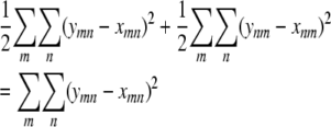subject to the constraints x_mm + x_nn = x_mn + x_nm for every pair {m, n}. It follows that diagonal blocks and off-diagonal blocks lead to the same constrained minimization problem.

appendix c shows that each of these least-squares problems has solution X = (x_mn) with residual

where Y = (y_mn), U = QYQ, and Q is the s × s projection matrix . In calculating a covariance, we can ignore symmetrization and replace the matrix by U. Indeed, the symmetry of C_ij implies that

Thus, tr(C_ijQΩ_klQ) faithfully represents the covariance between trait k of animal i and trait l of animal j. By the same reasoning, we can replace the entire residual matrix Ω − P(Ω) by the matrix

(14)

Here diag(Q) is a diagonal block matrix with all t diagonal blocks equal to Q. One can easily check that diag(Q) is a projection matrix and that R inherits the properties of symmetry and positive semidefiniteness from Ω.

In reparameterizing Ω, it is convenient to define an orthogonal matrix O mapping the vector to the standard basis vector e₁. (See appendix d for one version of O.) It follows that

Observe that pre- and postmultiplying any square matrix by zeros out the first row and first column of the matrix. To take advantage of this fact, we express the residual matrix (14) as

(15)

The matrix

is a positive semidefinite replacement for diag(O)Ω diag(O*). By our earlier remark, a block ϒ_kl of ϒ equals the corresponding block of diag(O)Ω diag(O*) with its first row and column zeroed out.

We are now close to the desired goal of reparameterizing the residual. The matrix ϒ has entire rows and columns consisting of zeros. Permuting its rows and columns appropriately will move its nontrivial part to an upper-left block, which will be positive definite whenever Ω is positive definite. The Cholesky decomposition of this upper-left block then serves as a good parameterization of R. To compute the number of parameters for s strains and t traits, observe that the matrix ϒ is st × st. A total of t rows and columns are lost in the zeroing-out process. This leaves an (st − t) × (st − t) upper-left block with (st − t)(st − t + 1)/2 diagonal or subdiagonal entries. For example, with three strains and two traits, there are 10 parameters.

For the sake of clarity, let us summarize how our proposed parameterization leads to trait covariances. It begins with a Cholesky decomposition Δ of an (st − t) × (st − t) positive definite matrix. The matrix ΔΔ* is then subdivided into (s − 1) × (s − 1) trait blocks (ΔΔ*)_kl, and each block is promoted to an s × s trait block ϒ_kl by adding a top row and left column of zeros. In matrix notation, ϒ_kl = Z(ΔΔ*)_klZ* with Z the s × (s − 1) matrix

Finally, we construct the residual matrix R via Equation 15, using the orthogonal matrix O.

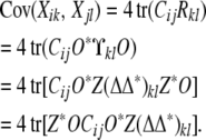
With these conventions, the covariance between trait k of animal i and trait l of animal j amounts to

(16)

In computing covariances over large pedigrees, it saves time and storage to precompute and store the (s − 1) × (s − 1) matrices 4Z*OC_ijO*Z and discard the s × s matrices C_ij. Note that the action A Z*AZ on an s × s matrix A deletes the first row and first column of A.

This ends our theoretical overview of the model. appendix e shows how to differentiate covariances with respect to parameters, and appendix f supplies a counterexample connecting identifiability and symmetry. We now move on to data analysis.

APPLICATIONS

A simulated advanced intercross line:

An AIL starts with F₁ offspring from an intercross of two inbred strains. The F₁ animals are randomly bred to produce the F₂ animals, the F₂ animals are randomly bred to produce the F₃ animals, and so on for a total of n generations. An AIL differs from repeated brother–sister mating, because it involves enough animals to preserve genetic diversity. It draws its strength from the steady accumulation of recombination events over many generations (Darvasi and Soller 1995). Simulating data according to an AIL design permits us to compare our mixed effects results with the fixed effects results of the benchmark program QTL Cartographer. This exercise is not meant to be a substitute for an exhaustive study of power and experimental design. Also, the comparison is not entirely fair because QTL Cartographer analyzes the F_n data at the last generation ignoring the previous generations. To reconstruct missing marker information, QTL Cartographer applies an inflated recombination fraction scaled to reflect n.

To create our simulated AIL data, we mated two inbred founder animals and subjected their descendants in each generation to virtual random mating. Generation 10 contained 175 animals in 140 sibships with 492 animals overall. Placing the QTL locus at the midpoint of markers 5 and 6 of 11 equally spaced marker loci, we simulated genotypes by gene dropping and assigned QTL effects on the basis of the genotypes at the QTL. QTL genotypes were then discarded from further analysis. We modeled a univariate trait with a grand mean η = 4, an environmental variance σ = 1, and a 2 × 2 polygenic variance matrix

For this simulated trait, strain one has a genetic variance comparable to the environmental variance and larger than the genetic variance of strain two. The two strains share a modest genetic correlation. For reasons explained in the next section, a single generation of data in a symmetric cross of this sort does not sustain estimation of strain-specific polygenic means. To circumvent this problem in our comparisons, we set the strain-specific polygenic means equal to 0. We chose small strain-specific QTL effects ɛ₁ = 0.2 and ɛ₂ = −0.2 centered around 0. In view of our discussion of identifiability, we can estimate only a single parameter p₁ characterizing Ω. The projection technique discussed yields the value p₁ = 0.667. The discussion of the C_ij matrices in appendix b explains why genotype data on a single generation also prevent estimation of p₁.

To provide the most informative comparisons, we ran three analyses: (1) Mendel on the full pedigree with complete genotype and phenotype data (Mendel Full), (2) Mendel on the full pedigree but with phenotype data on only the final F₁₀ generation (Mendel F₁₀), and (3) QTL Cartographer on the final F₁₀ generation with complete genotype and phenotype data (Cartographer). Simply comparing cases Mendel Full and Cartographer is hardly fair; the full pedigree contains more than twice the number of animals in the final generation. Mendel F₁₀ takes advantage of the full genealogy and all genotype data in computing theoretical and conditional strain coefficients. It limits itself to the phenotype sample in the last generation to enable a better comparison to QTL Cartographer.

Before turning to QTL mapping in the Mendel analyses, we fit a baseline model including the grand mean, the polygenic variance, and the environmental variance. We then estimated conditional strain coefficients at each of the 11 marker loci. This put us in a position to estimate the global parameters and the QTL-specific parameters simultaneously at each locus. The evidence in favor of the QTL is summarized by a likelihood ratio test (LRT) statistic following a distribution; a nonlinear false discovery rate (FDR) correction (Benjamini et al. 2001) corrects for multiple testing for all three analyses. Table 1 summarizes the type I error rate, power, and coverage as well as the generating parameters, their estimates, and the standard errors of the estimates at the loci adjacent to the QTL. Successful coverage occurs when the equivalent one-LOD drop interval (4.6 LRT units) includes the QTL. We reject the null hypothesis of no QTL effect when the LRT is significant at the 0.05 level.

The results in Table 1 reflect 100 simulations for a QTL-effect size that yields power >90% for Mendel Full; type I error rates are given as confidence intervals based on 500 simulations under the null hypothesis of no QTL effect. Clearly, the power to detect linkage is drastically reduced when only the F₁₀ generation is available for analysis. This absence of data also makes it difficult for Mendel F₁₀ to estimate the polygenic parameter p₁ accurately. For Mendel Full all estimates are within one standard error of their true values, and standard errors are small. QTL Cartographer exhibits slightly better power and coverage than Mendel F₁₀, but with a largely inflated type I error rate. Both methods are easily bested by Mendel Full. These trends continue over a range of smaller QTL effects (data not shown). We are pleased with these results. In our view they demonstrate that application of the mixed effects model sacrifices little in simple settings while generalizing readily to complex pedigrees.

A multivariate four-way cross:

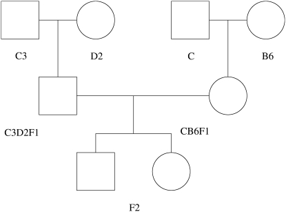
To illustrate the analysis of multivariate traits, we next consider the hormone data of Burke and colleagues (Harper et al. 2003) on aging UM-HET3 mice. Figure 1 shows how the UM-HET3 mice were created from four founder strains: BALB/cJ (C), C57BL/6J (B6), C3H/HeJ (C3), and DBA/2J (D2). CB6F₁ females crossed with C3D2F₁ males provided 967 F₂ full siblings. At markers with four different alleles, all F₂ mice were heterozygous. Thus compared to a two-way cross, the four-way cross doubles the number of founder strains without sacrificing phase certainty. Hormone levels of insulin-like growth factor I (IGF), leptin (Lep), and thyroxine (T4) were measured at 4 and 15 months on each of the F₂ mice. Testing maternal and paternal effects separately, Harper et al. found several linked markers in these data via ANOVA, including a maternal allele at D3Mit25 linked to IGF at 15 months, a paternal allele at D3Mit127 linked to Lep at 4 months, and both maternal and paternal alleles linked to Lep at 15 months. It is worth pointing out that ANOVA or MANOVA must be carried out at marker loci. Only here do marker genotypes or allele counts unambiguously define factor levels. With complete genotyping, our model collapses in this setting to the classical models.

Figure 1.—

Four-way cross for UM-HET3 Mice. UM-HET3 mice are created from four founder strains: BALB/cJ (C), C57BL/6J (B6), C3H/HeJ (C3), and DBA/2J (D2); the F₂ generation results from CB6F₁ females crossed with C3D2F₁ males.

This multistrain cross highlights identifiability pitfalls inherent in the structure of some crosses and the data collected on them. For example, all F₂ mice share the strain fraction vector . Hence, the polygenic mean is confounded with the grand mean. Using strain trait averages or phenotyping members of the original strains would allow us to estimate the polygenic means, but this is not an option for the current data.

Although the rigid structure of the four-way cross preserves phase certainty, it reduces uncertainty to the point where the polygenic covariance matrix cannot be estimated. Polygenic covariances depend on the combinatorial matrices C_ij. We have already noted that C_ij = 0 whenever i is a founder or i and j are F₁ mice. Straightforward calculations for F₂ mice i and j with i ≠ j yield

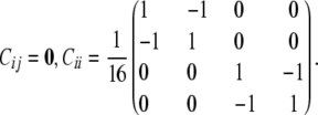Inspection of Equation 3 therefore shows that the polygenic covariance matrix Ω is confounded with the matrix describing the environmental covariances.

Finally, there are identifiability problems with the QTL allelic effects. At the covariance level, the conditional coefficient matrix is identically 0 when typing is full and different alleles are present in each strain. At the mean level, imposition of the constraint ɛ₄ = − ɛ₁ − ɛ₂ − ɛ₃ shows that the genotype-specific means in a purely allelic model can be expressed as the vector

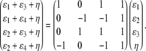Because the matrix on the right of this equation has less than full rank, some mean vectors are not representable. As a substitute for the additive QTL contributions, we assign a different mean effect to each of the four F₂ genotypes.

We analyze these data in the same manner as the simulated AIL except for graphing the −log₁₀(P-value) instead of LRTs and analyzing multiple map points in the intervals between marker loci. We enjoy two advantages over ANOVA or MANOVA; namely, we can use phenotyped individuals with wholly or partially missing genotypes, and we can estimate both QTL location and effect size.

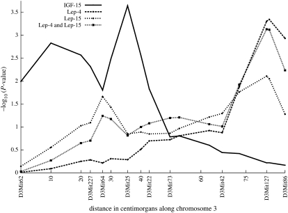
To carry out a multivariate analysis, one must decide which univariate traits to analyze together. This is not a trivial matter because combining traits exacerbates the multiple testing problem and may add noise and degrade power (Amos et al. 2001; Bauman et al. 2005). With outbred populations it is intertwined with the issue of ascertainment (Dawson and Elston 1984); it may also be a problem with inbred populations since strains are often chosen for a particular experiment on the basis of their average phenotype. We present here the results of two multivariate analyses making these points. The most interesting results from this example data set are on chromosome 3, and we focus on three traits, leptin measurements at both 4 and 15 months and insulin-like growth factor I at 15 months in this region. In univariate analysis, both IGF-15 and Lep-4 show significant linkage to markers on chromosome 3, while Lep-15 shows suggestive linkage. Multivariate analyses are indicated biologically, spatially, and temporally.

We carried out a number of multivariate analyses; some of the results are summarized in Figures 2 and 3 and Table 2. The graphs of −log₁₀(P-value) along chromosome 3 in Figure 2 correspond to the univariate analyses of IGF-15, Lep-4, and Lep-15 and the bivariate analysis of Lep-4 and Lep-15. The univariate graph of IGF-15 peaks over marker D3Mit5. Subjecting the P-values for IGF-15 to the nonlinear FDR correction (Benjamini et al. 2001) suggests a single location for IGF-15. Both of the univariate leptin graphs as well as the bivariate graph peak over D3Mit127. After FDR correction, at least two significant map points are suggested over D3Mit127 for the bivariate leptin analysis. Table 2 reports estimates and standard errors for the bivariate leptin mean parameters at marker D3Mit127. These estimates are very similar at the two time points. Although likelihood ratios improve over univariate analysis, P-values do not because the degrees of freedom of the χ² test double. The estimated environmental covariance matrix

(17)

is consistent with the raw correlation of the two traits. In the matrix (17), the standard error of each estimate appears in parentheses.

Figure 2.—

Univariate and bivariate results, four-way cross on chromosome 3, univariate results for IGF-15 peak over marker D3Mit25. Univariate and bivariate results for Lep-4 and Lep-15 peak over marker D3Mit127.

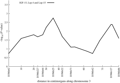
Figure 3.—

Trivariate analysis, four-way cross on chromosome 3, trivariate results peak over marker D3Mit25 and D3Mit86. These peaks are lower than those obtained with univariate and bivariate analyses.

A trivariate analysis of IGF-15, Lep-4, and Lep-15 clearly illustrates that in the case of multivariate traits, more is not always better. Comparing Figure 2 to Figure 3 shows two large peaks: one at marker D3Mit25 and one over marker D3Mit127. After FDR adjustment only the first peak survives, and the evidence for it is compromised. Thus, the trivariate analysis provides no additional linkage information and actually degrades the power to detect linkage. While leptin and IGF share numerous biological interactions, there is no evidence in these data for a common genetic determinant on chromosome 3.

An eight-strain simulated cross:

Our first two examples demonstrated the equivalence of the random effects model to the fixed effects model for standard cross designs and hint at the flexibility of our approach. To demonstrate this flexibility, we now present an eight-strain simulated example that (a) documents how correctly accounting for polygenic background can be beneficial and (b) demonstrates how it is possible to test hypotheses with the kind of unbalanced pedigree data encountered in human studies. As with the simulated AIL example, this exercise is not meant to be a substitute for an exhaustive study of power and experimental design.

Simulation specifics:

Our simulated cross involves a univariate trait, eight inbred strains, and seven pedigrees of nine generations each. We are motivated in part by the heterogeneous stock (Mott et al. 2000) and the collaborative-cross designs (Williams et al. 2002). Starting with strain-pure founders, we constructed each pedigree by random mating with a decreasing number of progeny per animal per generation. The average number of animals per pedigree is 366. Random mating ensures substantial diversity in theoretical and conditional strain fractions and coefficients. On the basis of the marker map for chromosome 2 in the UM-HET example of the previous section, we simulated genotypes at six loci using the gene-dropping option of Mendel. Locus 3 serves as the QTL and the remaining loci as markers. Genotypes at the QTL are omitted during linkage analysis.

We generated univariate trait values independently for each pedigree by sampling from a multivariate normal distribution with prescribed means and covariances. If animal i has QTL genotype a/b and trait value X_i, then

where η is the grand mean, μ is the vector of polygenic deviations from the mean, and ɛ is the vector of QTL deviations from the mean. For animals i and j, the polygenic and random environment contributions entail the covariance

Note the absence here of a QTL variance contribution. Although the data are analyzed conditionally given observed marker genotypes, they are generated unconditionally. Table 3 displays the values of the parameters used for the simulations. These values were chosen randomly subject to constraints such as .

TABLE 3.

Eight-strain cross: simulation generating parameters

Inbred strain a	μ(a)	ɛ(a)
BALB	−3.94	0.45
C57	5.62	0.24
C3H	−1.95	−0.24
DBA	2.13	−0.53
CAST	−3.68	−0.10
RIII	2.22	−0.68
I	−4.88	0.29
AKR	4.48	0.57
Grand	6.31	NA

Our simulation choices present both opportunities and challenges. For example, the fact that each strain is assigned a unique QTL allele suggests that even a simple F₂ cross between two strains would be adequate to map the QTL. This advantage is tempered by the long genetic distances separating the QTL from the flanking markers, by the smallness of the QTL effects, by the similarity of these effects in some strains, and by the discordance of the QTL effects and the polygenic means effects.

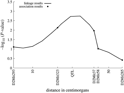
In using random effect models for QTL mapping, inclusion of polygenic background is usually a good idea. If polygenic background is present but ignored, then the only way of accounting for relative correlations is through the QTL component. When we analyze the current data omitting polygenic background, every single chromosome location in the linkage analysis achieves a P-value <0.00001. Adding polygenic background causes P-values to reach more reasonable levels, ranging from 0.0019 to 0.3835. Subjecting the P-values to the (FDR) procedure highlights the QTL and one neighboring point as significant (Benjamini et al. 2001). Figure 4 plots the function −log₁₀(P-value) along the chromosome; as earlier, the P-values reflect the likelihood ratio tests of the QTL component. The QTL is located at 30 cM from the origin between marker D2Mit323 at 23 cM and marker D2Mit37 at 42 cM.

Figure 4.—

Eight-strain cross example—linkage and association results for the simulated eight-strain random-mating example. Association results mirror linkage results at the markers. The linkage results peak over the QTL, located between markers D2Mit323 and D2Mit58.

We also used these data to illustrate the application of the QTL association model. As in our linkage analysis, omitting polygenic background leads to unrealistically small P-values. Figure 4 plots the −log₁₀(P-value) for the association analysis with the polygenic background. The association results are similar to the linkage results. The marker with the most significant result is D2Mit323, which is the marker nearest to the QTL. The FDR procedure singles out D2Mit323 as the only significant association.

Comparison of computation times between the two models illustrates the speed of the association analysis. The linkage model requires ∼4 hr for calculation of the coefficient matrices for each pedigree and ∼20 hr to estimate the parameters for each of the 17 points. The association model requires ∼1.5 hr for all calculations at each of the five markers.

DISCUSSION

In the hope of mapping QTL with small effects, geneticists are undertaking more ambitious crosses with multiple strains, multivariate traits, and dense marker sets. The random effects models developed here will enable a smooth transition to more sophisticated statistical analysis. The greatest strength of the models is their ability to capture polygenic background parsimoniously. A second strength is their versatility in handling large pedigrees, large numbers of contributing strains, and multivariate traits. While we have warned against importing ideas wholesale from the rest of statistical genetics, judicious adaptations are fully warranted. For example, since environment can be exquisitely controlled for inbred strain experiments, models of gene-by-environment interaction can be put to good use on the mean level (Blangero 1993) and on the variance level (Lange 1986; Itoh and Yamada 1990). These techniques apply both to continuous traits (Pletcher 1999; Pletcher and Geyer 1999; Jaffréic and Pletcher 2000; Pletcher and Jaffréic 2002; Purcell 2002; Purcell and Sham 2002; Meyer and Kirkpatrick 2005) and to categorical traits (Towne et al. 1997; Viel et al. 2005). It is also straightforward to model multiple QTL acting additively (Lange 2002).

Balanced against these strengths is the need for better-conceived study designs. Unless crosses are carefully structured, some parameters will be unidentifiable. One antidote is to scale back the complexity of a model and reparameterize. Our first two examples illustrate this tactic. Another antidote is to avoid monolithic designs and opt for a mixture of designs that individually reveal different features of a model. Our third example does this.

In random effects models, trait values for most animals are correlated. Logically, one should treat all animals as members of a single large pedigree. At some point this requirement becomes unwieldy. The computational demands of the random effects models are fairly high, so tactics such as pedigree splitting, marker thinning, and marker amalgamation should not be dismissed. It will probably take a combination of these tactics to cope with the large-scale mapping projects now under way (Pletcher et al. 2004). Fortunately, our experiences with simulated data suggest that a moderate amount of pedigree splitting sacrifices little information.

We have omitted a detailed discussion of how the program SimWalk delivers conditional strain fractions and coefficients. In our experience, SimWalk's MCMC algorithm adequately samples descent graph space. In association analysis, this lengthy process can be dispensed with if information at neighboring markers is ignored. Deterministic algorithms that produce approximate kinship and strain coefficients may ultimately be a better choice than stochastic sampling (Gao et al. 2004; Gao and Hoeschele 2005). In maximizing loglikelihoods, it is also worth mentioning that Mendel allows the user to set initial parameter values and bounds. This flexibility is valuable in exploring multimodal likelihood surfaces.

Our QTL parameters enter the model at both the mean and the variance level and are not subject to nonnegativity constraints. Thus, the asymptotic distribution of a likelihood ratio test follows a chi-square distribution with degrees of freedom equal to the difference in the number of independent parameters between the underlying nested models. Model selection can be accomplished by likelihood ratio tests or modified criteria such as the Akaike information criteria (AIC) or the Bayesian information criteria (BIC). Multiple testing is certainly an issue. The FDR correction of Benjamini and Hochberg (Benjamini et al. 2001) for dependent tests is often a useful cure and provided us with correct inferences in our simulated examples. Extensions such as Storey's optimal discovery procedure (Storey 2007; Storey et al. 2007) can lead to more accurate P-values and should be kept in mind.

The assumption of multivariate normality is helpful in maximum likelihood estimation. For univariate traits with excess kurtosis, the multivariate t distribution is a workable substitute for the multivariate normal distribution and is an implemented option in Mendel. It is reasonable to conjecture that some version of the central limit theorem should hold for a polygenic trait over a pedigree (Lange 1978; Lange and Boehnke 1983). For simple pedigrees generated en masse in a cross, one can check the normality assumption empirically. The impact of departures from normality has been considered by several researchers (Beaty et al. 1985; Allison et al. 1999; Pratt et al. 2000). Blangero et al. (2000) and Sham et al. (2000) suggest solutions to gross violations. One can object that QTL effects by their discrete nature cannot be normal. Three responses are possible. First, this objection has never stopped ordinary QTL mapping with outbred populations. Second, under the null hypothesis, the discrete effects disappear. Third, in all but the simplest crosses, application of a rigorous model incorporating both polygenes and major genes is very computationally demanding.

The web site (http://www.genetics.ucla.edu/software) offers the current versions of Mendel and SimWalk for several computing platforms. Ample documentation and sample problems are provided. The experimental versions of Mendel and SimWalk featured in this article will be released publicly as soon as it is practical.

APPENDIX A: REPRESENTATION OF POSITIVE DEFINITE MATRICES

Given a k × k positive definite matrix Ω and a k × 1 vector μ, we now prove that vectors μ₁, … , μ_n exist such that and . To simplify the proof, we pass to the spectral decomposition Ω = O*DO of Ω. Here O is an orthogonal matrix, and D is a diagonal matrix whose jth diagonal entry d_j is an eigenvalue of Ω. If n vectors ν₁, … , ν_n exist such that and , then taking μ_i = O*ν_i for each i completes the proof.

With the transformed problem, we can work on each dimension j separately. Suppose we can find scalars a₁, … , a_m such that a₁ + … + a_m = ν_j and + … + = d_j. Then we construct m vectors w₁, … , w_m whose entries are 0 except for their jth entries w_ij = a_i. These m vectors compose part of the solution set ν₁, … , ν_n and do not impinge on the parts contributed by other dimensions. To show that appropriate scalars a₁, … , a_m exist, we consider optimizing the function f(a) = + … + subject to the affine constraint a₁ + … + a_m = ν_j. By introducing a Lagrange multiplier, we can prove that f(a) attains its minimum when all a_i = ν_j/m. The maximum of f(a) is infinite in all but the trivial case m = 1. For instance, we can take , , and all other a_i = 0 and send p to ∞. Since d_j must be positive, some positive integer m exists with < d_j. This choice of m puts us in a position to invoke the intermediate value theorem. The set of vectors a = (a₁, … , a_m) satisfying the constraint is convex and therefore connected. A continuous function on a connected set attains every value between its minimum and maximum values. Hence, there is some a with f(a) = d_j.

APPENDIX B: PROPERTIES OF THE C_IJ MATRICES

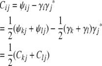
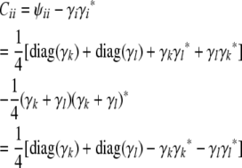
The role of the matrix C_ij in formula (3) suggests its importance. Mathematically C_ij is better behaved than the strain coefficient matrix ψ_ij. Recall that the founder initial conditions and the recurrences (4)–(7) completely determine the strain fraction vectors γ_i and the strain coefficient matrices ψ_ij. If we retain the conventions that i has parents k and l and j is an animal previously considered, then the last three recurrences translate into the similar recurrences

(B1)

(B2)

and

(B3)

on the C_ij matrices. The next proposition collects some relevant facts.

Proposition 1. In addition to satisfying the recurrences (B1), (B2), and (B3), the matrix C_ij

1. has all entries 0 when either i or j is a founder,

2. is symmetric,

3. is positive semidefinite,

4. has the vector 1 in its null space,

5. has entries C_ij(m, n) confined to the interval for n ≠ m and to the interval for n = m.

Proof.

1. If i is a founder belonging to strain q and j is a founder belonging to strain r, then by definition γ_i(m) = 1_{m=q}, γ_j(n) = 1_{n=r}, and ψ_ij(m, n) = 1_{m=q}1_{n=r}. Thus, all entries of C_ij vanish. If i or j is a founder but the other is not, then induction and the recurrences (B1) and (B2) show that all entries of C_ij vanish.

2. Formula (B3) forces C_ii to be symmetric, and the recurrences (B1) and (B2) preserve symmetry.

3. Because the recurrences (B1) and (B2) preserve positive semidefiniteness, it suffices to prove that C_ii is positive semidefinite. Inspection of formula (B3) further demonstrates that it suffices to prove that diag(γ_k) − γ_kγ_k* is positive semidefinite for all k. Accordingly, let v be an arbitrary vector. The quadratic form

   

   is nonnegative owing to Cauchy's inequality

   

   and the fact that .
4. Again this is a consequence of the recurrences (B1) and (B2) and the validity of the assertion for C_ii. In the latter case, the equality

   

   is obvious.

5. Because the stated bounds are preserved by recurrences (B1) and (B2), it suffices to consider C_ii. The contribution to a diagonal term in Equation B3 is bounded below by 0 and above by . The contribution to an off-diagonal term is bounded below by and above by 0. ▪

The collection 𝒞 of all C_ij matrices over a pedigree has considerable structure. For example, the symmetry of C_ij entails C_ij = C_ji. With just s = 2 strains, parts b, d, and e of Proposition 1 imply that every C_ij is representable as

for some constant . Furthermore, since a_ij = 0 whenever i or j is a founder or an F₁ individual, straightforward recursive arguments show that within any strictly linear mating designs like F_n, a_ij = 0 for all i ≠ j. Two-strain systems also produce uninteresting conditional coefficients; straightforward calculations show that for all i and j at markers that differentiate between the strains with complete genotyping.

To generalize this representation to more than two strains, it is helpful to introduce the s × s matrix E_mn where all entries of E_mn are 0 except for e_mm = e_nn = 1 and e_mn = e_nm = −1. There are such matrices.

Proposition 2. Every matrix C_ij from the collection 𝒞 can be represented as a linear combination

(B4)

Furthermore, the coefficients a_ij,mn are nonnegative dyadic rationals satisfying

Proof. Each matrix C_ii = 0 corresponding to a founder i clearly qualifies. The representation (B4) is preserved by the averaging process of the recurrences (B1) and (B2), so it suffices to prove the representation for a matrix C_ii generated by a nonfounder. Again the averaging nature of recurrence (B3) allows us to verify the representation (B4) for a matrix of the form . Because the set of dyadic rationals constitutes an algebraic field, it is clear by induction that all entries of γ_k are dyadic rationals. We now claim that

(B5)

Equality (B5) is certainly true for the off-diagonal entries of the matrices on both sides. For the diagonal entries, it is a consequence of the identity

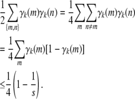
Because the coefficients are dyadic rationals, all that remains is to check that the sum of the coefficients is properly bounded. This follows from

(B6)

The upper bound (B6) can be proved by introducing a Lagrange multiplier corresponding to the constraint . Equality is achieved only when all . ▪

APPENDIX C: COMPUTATION OF THE PROJECTION

Consider minimizing the function

subject to the constraints x_mm + x_nn = x_mn + x_nm for every unordered pair {m, n}. We proceed by seeking a stationary point of the Lagrangian

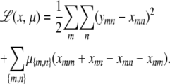This point is characterized by the equations

(C1)

(C2)

with the convention that m ≠ n. Rearrangement of Equation (C1) gives

(C3)

If we interchange m and n in Equation C3, add the result to Equation C3, and invoke the constraint (C2), then we get the equation

determining μ_{m,n} as

From Equation C3 it follows that

(C4)

It is easy to check that the constraint (C2) is implicit in this solution. Furthermore, the solution entails the residual

If we set , our objective function can now be expressed as

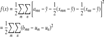
Neither the off-diagonal entries x_mn nor the constraints now appear. To solve this unconstrained problem, we center the a_mn by subtracting their average value . This allows us to reparameterize f(x) as

in more or less obvious notation.

Minimizing the objective function in this form coincides with a classical problem in population genetics. If we assume that m and n represent two possible alleles from s equally frequent alleles and b_mn represents a trait value determined by the genotype m/n, then minimizing f(x) corresponds to the problem of determining the additive genetic variance of a centered trait. The solution to this problem is known to be

It follows that

A final substitution for a_mn gives

and the general formula

(C5)

based on Equation (C4) and valid for both m ≠ n and m = n.

The projection solution (C5) reduces the residual r_mn = y_mn − x_mn to

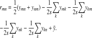If we define a matrix R with entries r_mn and a matrix U with entries

then it is clear that

In other words, the residual matrix is a symmetrized version of U. Fortunately, we can represent U as the matrix product

of Y = (y_mn) sandwiched between two copies of the orthogonal projection .

APPENDIX D: CONSTRUCTION OF AN ORTHOGONAL MATRIX

An orthogonal matrix O mapping the vector to the standard basis vector e₁ can be explicitly constructed by the Gramm–Schmidt process applied to the basis , where e_k is the standard basis vector with 1 in position k and zeros elsewhere. The first row of O is just ; the subsequent rows take the form

where k − 2 zeros precede the entry s − k + 1. The reader can easily check that the row vectors provide an orthonormal basis.

APPENDIX E: DIFFERENTIATION OF VARIANCES AND COVARIANCES

Because the fastest maximum likelihood algorithms rely on exact derivatives, there is an obvious need to calculate the partial derivatives of each covariance Cov(X_ik, X_jl) with respect to the entries of Δ = (δ_mn). If we let ∂_mn denote partial differentiation with respect to δ_mn, then formula (16) immediately leads to

so it suffices to compute the partial derivatives of ΔΔ* = (d_uv). Since

the product rule of differentiation yields

Thus, ∂_mn(ΔΔ*) consists entirely of zeros except for row m and column n. This fact considerably simplifies computation of derivatives.

APPENDIX F: A COUNTEREXAMPLE ON IDENTIFIABILITY

Finally, we consider a counterexample that illustrates some of the subtleties of identifiability. We noted that projection replaces each trait block Y = Ω_kl with a symmetrized block residual

For purposes of computing covariances, we argued that symmetrization is unnecessary and avoiding it simultaneously yields correct covariances and reduces the number of parameters. We have not actually demonstrated that no further reduction is possible. Furthermore, exploiting the symmetrized version may lead to a residual Ω − P(Ω) that fails to be positive semidefinite. Consider the matrix

Straightforward algebra leads to the positive semidefinite matrix

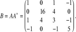If we symmetrize each 2 × 2 block of B, then we get

A tedious computation shows that

and C cannot be positive semidefinite.

References

- Allison, D. B., M. C. Neale, R. Zannolli, N. J. Schork, C. I. Amos et al., 1999. Testing the robustness of the likelihood-ratio test in a variance-component quantitative-trait loci-mapping procedure. Am. J. Hum. Genet. 65 531–544. [DOI] [PMC free article] [PubMed] [Google Scholar]
- Amos, C. I., 1994. Robust variance-components approach for assessing genetic linkage in pedigrees. Am. J. Hum. Genet. 54 535–543. [PMC free article] [PubMed] [Google Scholar]
- Amos, C. I., M. de Andrade and D. K. Zhu, 2001. Comparison of multivariate tests for genetic linkage. Hum. Hered. 51 133–144. [DOI] [PubMed] [Google Scholar]
- Bauman, L. E., L. Almasy, J. Blangero, R. Duggirala, J. Sinsheimer et al., 2005. Fishing for pleiotropic QTLs in a polygenic sea. Ann. Hum. Genet. 69 590–611. [DOI] [PubMed] [Google Scholar]
- Beaty, T. H., S. G. Self, K.-Y. Liang, M. A. Connolly, G. A. Chase et al., 1985. Use of robust covariance components models to analyse triglyceride data in families. Ann. Hum. Genet. 49 315–328. [DOI] [PubMed] [Google Scholar]
- Benjamini, Y., D. Drai, G. Elmer, N. Kafkafi and I. Golani, 2001. Controlling the false discovery rate in behavior genetics research. Behav. Brain Res. 125 279–284. [DOI] [PubMed] [Google Scholar]
- Blangero, J., 1993. Statistical approaches to human adaptability. Hum. Biol. 65 941–966. [PubMed] [Google Scholar]
- Blangero, J., and L. Almasy, 1997. Multipoint oligogenic linkage analysis of quantitative traits. Genet. Epidemiol. 14 959–964. [DOI] [PubMed] [Google Scholar]
- Blangero, J., J. T. Williams and L. Almasy, 2000. Robust lod scores for variance component-based linkage analysis. Genet. Epidemiol. 19 S8–S14. [DOI] [PubMed] [Google Scholar]
- Broman, K. W., H. Wu, Ś. Sen and G. A. Churchill, 2003. R/qtl: QTL mapping in experimental crosses. Bioinformatics 19 889–890. [DOI] [PubMed] [Google Scholar]
- Cervino, A. C. L., A. Darvasi, M. Fallahi, C. C. Mader and N. F. Tsinoremas, 2007. An integrated in silico gene mapping strategy in inbred mice. Genetics 175 321–333. [DOI] [PMC free article] [PubMed] [Google Scholar]
- Churchill, G. A., and R. W. Doerge, 1994. Empirical threshold values for quantitative trait mapping. Genetics 138 963–971. [DOI] [PMC free article] [PubMed] [Google Scholar]
- Darvasi, A., and M. Soller, 1995. Advanced intercross lines, an experimental population for fine genetic mapping. Genetics 141 1199–1207. [DOI] [PMC free article] [PubMed] [Google Scholar]
- Dawson, D. V., and R. C. Elston, 1984. A bivariate problem in human-genetics—ascertainment of families through a correlated trait. Am. J. Med. Genet. 18 435–448. [DOI] [PubMed] [Google Scholar]
- Flint, J., W. Valdar, S. Shifman and R. Mott, 2005. Strategies for mapping and cloning quantitative trait genes in rodents. Nat. Rev. Genet. 6 271–286. [DOI] [PubMed] [Google Scholar]
- Gao, G., and I. Hoeschele, 2005. Approximating identity-by-descent matrices using multiple haplotype configurations on pedigrees. Genetics 171 365–376. [DOI] [PMC free article] [PubMed] [Google Scholar]
- Gao, G., I. Hoeschele, P. Sorensen and F. Du, 2004. Conditional probability methods for haplotyping in pedigrees. Genetics 167 2055–2065. [DOI] [PMC free article] [PubMed] [Google Scholar]
- Goldgar, D. E., 1990. Multipoint analysis of human quantitative genetic-variation. Am. J. Hum. Genet. 47 957–967. [PMC free article] [PubMed] [Google Scholar]
- Haley, C. S., and S. A. Knott, 1992. A simple regression method for mapping quantitative trait loci in line crosses using flanking markers. Heredity 69 315–324. [DOI] [PubMed] [Google Scholar]
- Harper, J. M., A. T. Galecki, D. T. Burke, S. L. Pinkosky and R. A. Miller, 2003. Quantitative trait loci for insulin-like growth factor I, leptin, thyroxine, and corticosterone in genetically heterogeneous mice. Physiol. Genomics 15 44–51. [DOI] [PubMed] [Google Scholar]
- Hitzemann, R. W., B. Malmanger, S. Cooper, S. Coulombe, C. Reed et al., 2002. Multiple cross mapping (MCM) markedly improves the localization of a QTL for ethanol-induced activation. Genes Brain Behav. 1 214–222. [DOI] [PubMed] [Google Scholar]
- Hopper, J. L., and J. D. Mathews, 1982. Extensions to multivariate normal models for pedigree analysis. Ann. Hum. Genet. 46 373–383. [DOI] [PubMed] [Google Scholar]
- Itoh, Y., and Y. Yamada, 1990. Relationships between genotype x environment interaction and genetic correlation of the same trait measured in different environments. Theor. Appl. Genet. 80 11–16. [DOI] [PubMed] [Google Scholar]
- Jaffréic, F., and S. D. Pletcher, 2000. Statistical models for estimating the genetic basis of repeated measures and other function-valued traits. Genetics 156 913–922. [DOI] [PMC free article] [PubMed] [Google Scholar]
- Janninka, J.-L., and R. Jansena, 2001. Mapping epistatic quantitative trait loci with one-dimensional genome searches. Genetics 157 445–454. [DOI] [PMC free article] [PubMed] [Google Scholar]
- Kao, C.-H., Z.-B. Zeng and R. D. Teasdale, 1999. Multiple interval mapping for quantitative trait loci. Genetics 152 1203–1216. [DOI] [PMC free article] [PubMed] [Google Scholar]
- Kruglyak, L., M. J. Daly, M. P. Reeve-Daly and E. S. Lander, 1996. Parametric and nonparametric linkage analysis: a unified multipoint approach. Am. J. Hum. Genet. 58 1347–1363. [PMC free article] [PubMed] [Google Scholar]
- Lander, E. S., and D. Botstein, 1989. Mapping Mendelian factors underlying quantitative traits using RFLP linkage maps. Genetics 121 185–199. [DOI] [PMC free article] [PubMed] [Google Scholar]
- Lange, K., 1978. Central limit theorems for pedigrees. J. Math. Biol. 6 59–66. [Google Scholar]
- Lange, K., 1986. Cohabitation, convergence and environmental covariances. Am. J. Med. Genet. 24 483–491. [DOI] [PubMed] [Google Scholar]
- Lange, K., 2002. Mathematical and Statistical Methods for Genetic Analysis, Ed. 2. Springer-Verlag, New York.
- Lange, K., and M. Boehnke, 1983. Extensions to pedigree analysis. IV. Covariance components models for multivariate traits. Am. J. Med. Genet. 14 513–524. [DOI] [PubMed] [Google Scholar]
- Lange, K., J. S. Sinsheimer and E. M. Sobel, 2005. Association testing with Mendel. Genet. Epidemiol. 29 36–50. [DOI] [PubMed] [Google Scholar]
- Li, R., M. A. Lyons, H. Wittenburg, B. Piagen and G. A. Churchill, 2005. Combining data from multiple inbred line crosses improves the power and resolution of quantitative trait loci mapping. Genetics 169 1699–1709. [DOI] [PMC free article] [PubMed] [Google Scholar]
- Liu, Y., and Z.-B. Zeng, 2000. A general mixture model approach for mapping quantitative trait loci from diverse cross designs involving multiple inbred lines. Genet. Res. 75 345–355. [DOI] [PubMed] [Google Scholar]
- Manly, K. F., and J. M. Olson, 1999. Overview of QTL mapping software and introduction to Map Manager QT. Mamm. Genome 10 327–334. [DOI] [PubMed] [Google Scholar]
- Meyer, K., and M. Kirkpatrick, 2005. Up hill, down dale: quantitative genetics of curvaceous traits. Philos. Trans. R. Soc. 360 1443–1455. [DOI] [PMC free article] [PubMed] [Google Scholar]
- Mott, R., C. J. Talbot, M. G. Turri, A. C. Collins and J. Flint, 2000. A method for fine mapping quantitative trait loci in outbred animal stocks. Proc. Natl. Acad. Sci. USA 97 12649–12654. [DOI] [PMC free article] [PubMed] [Google Scholar]
- Pletcher, M. T., P. McClurg, S. Batalov, A. I. Su, S. W. Barnes et al., 2004. Use of a dense single nucleotide polymorphism map for in silico mapping in the mouse. PLoS Biol. 2 2159–2169. [DOI] [PMC free article] [PubMed] [Google Scholar]
- Pletcher, S. D., 1999. Model fitting and hypothesis testing for age-specific mortality data. J. Evol. Biol. 12 430–439. [Google Scholar]
- Pletcher, S. D., and C. J. Geyer, 1999. The genetic analysis of age-dependent traits: modeling the character process. Genetics 153 825–835. [DOI] [PMC free article] [PubMed] [Google Scholar]
- Pletcher, S. D., and F. Jaffréic, 2002. Generalized character process models: estimating the genetic basis of traits that cannot be observed and that change with age or environmental conditions. Biometrics 58 157–162. [DOI] [PubMed] [Google Scholar]
- Pratt, S. C., M. J. Daly and L. Kruglyak, 2000. Exact multipoint quantitative-trait linkage analysis in pedigrees by variance components. Am. J. Hum. Genet. 6 1153–1157. [DOI] [PMC free article] [PubMed] [Google Scholar]
- Purcell, S., 2002. Variance components models for gene-environment interaction in twin analysis. Twin Res. 5 554–571. [DOI] [PubMed] [Google Scholar]
- Purcell, S., and P. Sham, 2002. Variance components models for gene-environment interaction in quantitative trait locus linkage analysis. Twin Res. 5 572–576. [DOI] [PubMed] [Google Scholar]
- Rebai, A., and B. Goffinet, 1993. Power of tests for QTL detection using replicated progenies derived from a diallel cross. Theor. Appl. Genet. 86 1014–1022. [DOI] [PubMed] [Google Scholar]
- Schork, N. J., 1993. Extended multipoint identity-by-descent analysis of human quantitative traits: efficiency, power, and modeling considerations. Am. J. Hum. Genet. 53 1306–1319. [PMC free article] [PubMed] [Google Scholar]
- Seaton, G., C. S. Haley, S. A. Knott, M. Kearsey and P. M. Visscher, 2002. QTL Express: mapping quantitative trait loci in simple and complex pedigrees. Bioinformatics 18 339–340. [DOI] [PubMed] [Google Scholar]
- Sen, Ś., and G. A. Churchill, 2001. A statistical framework for quantitative trait mapping. Genetics 159 371–387. [DOI] [PMC free article] [PubMed] [Google Scholar]
- Sham, P. C., J. H. Zhao, S. S. Cherny and J. K. Hewitt, 2000. Variance-components QTL linkage analysis of selected and non-normal samples: conditioning on trait values. Genet. Epidemiol. 19 S22–S28. [DOI] [PubMed] [Google Scholar]
- Sillanpää, M. J., and E. Arjas, 1998. Bayesian mapping of multiple quantitative trait loci from incomplete inbred line cross data. Genetics 148 1373–1388. [DOI] [PMC free article] [PubMed] [Google Scholar]
- Sobel, E. M., and K. Lange, 1996. Descent graphs in pedigree analysis: applications to haplotyping, location scores, and marker-sharing statistics. Am. J. Hum. Genet. 58 1323–1337. [PMC free article] [PubMed] [Google Scholar]
- Storey, J. D., 2007. The optimal discovery procedure: a new approach to simultaneous significance testing. J. R. Stat. Soc. B 69 347–368. [Google Scholar]
- Storey, J. D., J. Y. Dai and J. T. Leek, 2007. The optimal discovery procedure for large-scale significance testing, with applications to comparative microarray experiments. Biostatistics 8 414–432. [DOI] [PubMed] [Google Scholar]
- Towne, B., R. M. Siervogel and J. Blangero, 1997. Effects of genotype-by-sex interaction on quantitative trait linkage analysis. Genet. Epidemiol. 14 1053–1058. [DOI] [PubMed] [Google Scholar]
- Valdar, W., J. Flint and R. Mott, 2006. Simulating the collaborative cross: power of quantitative trait loci detection and mapping resolution in large sets of recombinant inbred strains of mice. Genetics 172 1783–1797. [DOI] [PMC free article] [PubMed] [Google Scholar]
- Viel, K. R., D. M. Warren, A. Buil, T. D. Dyer, T. E. Howard et al., 2005. A comparison of discrete versus continuous environment in a variance components-based linkage analysis of the COGA data. BMC Genet. 6(Suppl. 1): S57. [DOI] [PMC free article] [PubMed] [Google Scholar]
- Williams, R. W., K. W. Broman, J. M. Cheverud, G. A. Churchill, R. W. Hitzemann et al., 2002. A collaborative cross for high-precision complex trait analysis. First workshop report of the complex trait consortium. Technical report.
- Xie, C., D. D. G. Gessler and S. Xu, 1989. Combining different line crosses for mapping quantitative trait loci using the identical by descent-based variance component method. Genetics 149 1139–1146. [DOI] [PMC free article] [PubMed] [Google Scholar]
- Zeng, Z.-B., 1993. Theoretical basis for separation of multiple linked gene effects in mapping quantitative trait loci. Proc. Natl. Acad. Sci. USA 90 10972–10976. [DOI] [PMC free article] [PubMed] [Google Scholar]
- Zeng, Z.-B., 1994. Precision mapping of quantitative trait loci. Genetics 136 1457–1468. [DOI] [PMC free article] [PubMed] [Google Scholar]