Bioinspired Methodology for Artificial Olfaction

Abstract

Artificial olfaction is a potential tool for noninvasive chemical monitoring. Application of “electronic noses” typically involves recognition of “pretrained” chemicals, while long-term operation and generalization of training to allow chemical classification of “unknown” analytes remain challenges. The latter analytical capability is critically important, as it is unfeasible to pre-expose the sensor to every analyte it might encounter. Here, we demonstrate a biologically inspired approach where the recognition and generalization problems are decoupled and resolved in a hierarchical fashion. Analyte composition is refined in a progression from general (e.g., target is a hydrocarbon) to precise (e.g., target is ethane), using highly optimized response features for each step. We validate this approach using a MEMS-based chemiresistive microsensor array. We show that this approach, a unique departure from existing methodologies in artificial olfaction, allows the recognition module to better mitigate sensor-aging effects and to better classify unknowns, enhancing the utility of chemical sensors for real-world applications.

Biological olfactory systems have the extraordinary ability to demonstrate reliable recognition of odorants over long time scales and to classify new odorants based upon chemical similarity to those that have been previously learned. Inspired by the olfactory system, artificial devices that combine arrays of chemical sensors with pattern recognition techniques, commonly termed “electronic noses”, have been explored for use as inexpensive chemical point detectors.^1–5 There is increasing demand for such devices to fill vital roles in medical diagnostics, homeland security, industrial process control, and other areas. In spite of their high potential for use in a variety of applications, these devices have achieved only limited success, largely due to variability in sensor output, which affects recognition of odorants over time, and a lack of methods to allow generalization of training to new analytes. These two issues are at the core of chemical sensor research.

Correct recognition of a specific chemical requires detection, in some way, of an aspect of the molecular features unique to that analyte. On the other hand, generalization to unknown chemical species requires detection of features that are common across a desired class of analytes. The opposing nature of these constraints suggests that achieving both capabilities requires a multistep chemical identity resolution process. This is in opposition to the conventional, one step (“all-at-once”) procedure that has been used in engineered chemical sensors to date.^6–11 Furthermore, for practical use, chemical sensors must be able to cope with variability in sensor responses due to various sources of aging.¹² Such aging potentially leads to misalignment between sensor measurements during operation and the chemical finger-prints registered during training, thereby impeding recognition of analytes.

How does the biological olfactory system deal with these conflicting analytical tasks? Odorant molecules that enter nostrils bind with olfactory receptor neurons in the olfactory epithelium that transduce the chemical stimuli into an electrical neural signal. The biological system incorporates both redundancy (multiple copies of each type of sensory neuron) and diversity (multiple types of sensory neurons depending on the gene they express) to detect chemicals.¹³ A given odorant, whether it is a pure analyte or a complex mixture, evokes a combinatorial response across a large population of sensory neurons.¹⁴ The high-dimensional inputs from the sensory neurons are subsequently transformed by neural circuits such that initially coarse odor representation is increasingly refined over time to become more odor-specific.¹⁵ The segmentation of odor class and identity information is done in a hierarchical fashion.

Here, we adapt this elegant divide-and-conquer biological approach to solve a parallel engineering problem in artificial olfaction and demonstrate its viability using a microelectromechanical system (MEMS)-based microhotplate array with metal oxide chemiresistors. We note, however, that the approach is applicable to any sensor array that yields analytically rich data. The response of each microelement at a select temperature is treated as a separate “pseudo”¹⁶ or “virtual” sensor¹⁷ to generate a high-dimensional chemical representation (5600 sensor–temperature pairs) that qualitatively mimics the combinatorial nature of the input from sensory neurons. By selecting (using the training data) a subset of sensor responses from these analytically rich data sets to initially perform discrimination of broad chemical classes, and progressively refining the selected data subset to allow finer discrimination between members within a class, we demonstrate robust recognition and generalization capabilities during validation testing. We also show that the proposed bioinspired approach is less sensitive to sensor aging compared to traditional approaches, thereby allowing sensing devices to remain functional for extended periods of operation.

EXPERIMENTAL SECTION

We used a 16-element MEMS microhotplate chemical sensor array^18,19 (see Figure 1) for our experiments. Each microhotplate includes an independently controlled, polysilicon electrical heating line and a thin-film, metal oxide semiconductor sensor material. SnO₂ and TiO₂ sensor materials (some pure, some layered, and some with ruthenium dopant) were placed on individual elements by a thermal, self-lithographic chemical vapor deposition technique.¹⁸ In addition, WO₃ sensors were produced by micropipetting and then thermally decomposing a peroxytungstate solution on two of the microhotplates. The resulting films populate a 16-element array as shown in Supporting Information, Figure S-1.

Figure 1.

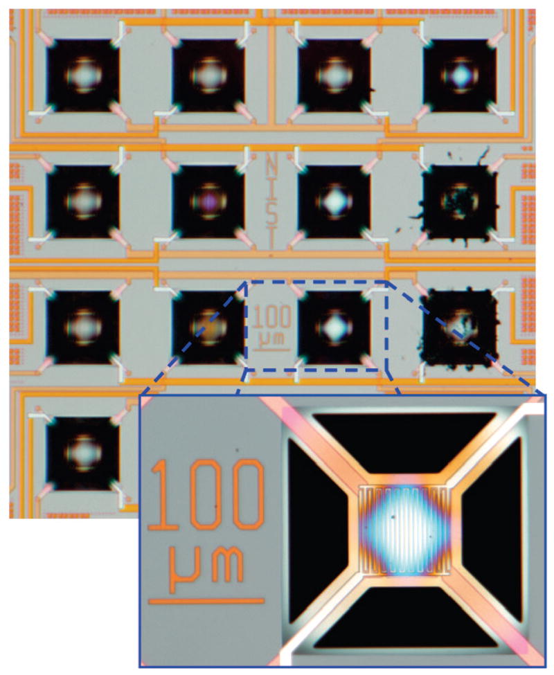
Optical micrographs of the microhotplate sensors. A 16-element array is shown in the upper portion, and a magnified view of one of the elements is shown in the lower portion. Bright features on the microhotplates are the platinum interdigitated electrodes that electrically contact the sensing films. Coloration of the microhotplates comes from optical interference caused by the sensing films. Dark regions indicate the micromachined etch pit that provides thermal isolation.

To generate the required analytical information, we also enriched the outputs of each microelement along a key chemical dimension, i.e., temperature, to probe thermodynamics and kinetics of interactions between the sensor and its environment. During the training and testing stages, sensors were operated using a ramp from 50 to 500 °C, with a ramp rate of ≈5 °C/s. Conductance measurements were made for each sensor in 1 °C increments. Immediately before the beginning of each ramp, a sensor was held at 500 °C for 2 s to provide a “burnoff” period. The measurements between 50 and 150 °C were often noisy and thus ignored. A total of 16 sensors and 350 temperatures per ramp resulted in an extremely complex and feature-rich data set.

The background of all measurements was flowing, zero-grade dry air. Added to this background were the analytes, added one at a time and in random order. Each analyte except water was diluted to 3 μmol/mol. Water was presented at 100 μmol/mol. Methanol and propane were additionally presented during training at concentrations ranging from 30 nmol/mol to 10 μmol/mol. The total flow rate across the sensor was a constant 1 standard L/min.

Analytes used during the training were as follows: three simple oxides (water, carbon monoxide, carbon dioxide); two alcohols (methanol, ethanol); two ketones (acetone, methyl ethyl ketone); two alkanes (ethane, propane) and two aromatics (benzene, toluene). The molecular structures of these analytes are given in Supporting Information, Figure S-2. Between each analyte, the sensor was returned to dry air. The output of the sensor was relatively constant after a transition of two to three measurement cycles following the introduction or removal of an analyte. These initial, transitional measurements were removed from the training set.

Between the training and testing stages, the sensor was subjected to an accelerated aging protocol. For 24 h, the sensors were intermittently held at 500 °C, rapidly thermally cycled, and exposed to methanol and propane. After this, the embedded heaters were recalibrated. These processes were intended to cause drift in the sensors through various means.

During the test phase, the sensor was operated as before, exposing it to some of the analytes seen in the training set: methanol, acetone, ethane, and benzene. In addition, four new analytes not included in the training set were presented to the sensor array: two alcohols (1-propanol, 2-propanol) and two ketones (methyl isobutyl ketone, cyclohexanone). Note that the new analytes are more complex and, other than the defining functional group presence, structurally quite different from the model analytes used in the training set (see Supporting Information, Figure S-2). These aspects were specifically selected as a challenge to our classification approach. Replicating the training-phase protocol, the sensor was returned to dry air between different analytes; however, the task of detecting a chemical event from a nonevent (dry air) was also assigned to the recognition module to simulate a real-time test.

All data analyses were done using custom routines written in a commercial, matrix-based mathematics software package. A differential approach was used to mitigate drift in an online, unsupervised manner. In this approach, the relative change in conductance, G, with respect to the conductance at 150 °C, G₀, was considered as the drift-corrected sensor response, G′

$$G^{\prime }=\frac{logG-log{G}_0}{log{G}_0}$$ (1)

Since the baseline response was determined separately for each measurement and for each sensing material, this simple approach accounted for the variable amount of drift for different materials and different analytes, as seen in Supporting Information, Figure S-3.

RESULTS AND DISCUSSION

Conventional, All-at-Once Approaches

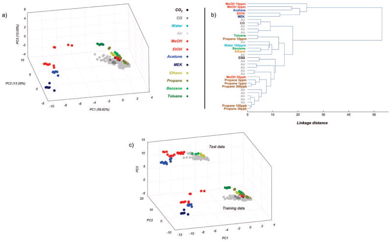
We first analyzed the training data using two all-at-once approaches that have been extensively used for analyte recognition in previous sensing studies: principal components analysis (PCA) and hierarchical clustering analysis (HCA).^8,9,20–22 We used PCA to visualize the high-dimensional sensor array data (16 sensors × 350 temperatures).²³ The multidimensional sensor responses were projected onto the first two or three dimensions, defined by the first few eigenvectors (sorted starting with the largest eigenvalue) of the response covariance matrix that captures most of the variance in the data set. We normalized each sensor response to its maximum conductance value in order to obtain PCA projections that favor separation of the analytes independent of their concentrations. Figure 2a shows the projection of the 5600-dimensional sensor array response to different training analytes along the first three principal components. Each point represents the sensor response to a particular analyte. As can be clearly seen, sensor responses to a given analyte are well clustered. However, analytes that have overlapping chemical features (e.g., the same functional group) do not necessarily group together to form superclusters. Further, the dry air responses do not form a single, well-defined cluster, indicating drift in sensor response over time even within the training period. This variability of sensor response to dry air samples makes reliable detection of some analytes like CO, benzene, and ethane extremely difficult.

Figure 2.

Conventional, all-at-once approaches to classification of the training data. (a) PCA, projecting the training data along the three principal directions that accounted for the maximum variance. Each sphere represents one measurement during the training phase. The color uniquely identifies the analyte to which the sensor array was exposed during the measurement: dark green, toluene; light green, benzene; dark yellow, propane; light yellow, ethane; dark blue, methyl ethyl ketone; light blue, acetone; dark red, methanol; light red, ethanol light gray, dry air, cyan, water; dark gray, CO; black, CO₂. (b) HCA of the same data, using the mean value of the response in each analyte. (c) PCA scatter plot showing both the training and testing data along the three principal directions of variance in the training data.

To quantitatively evaluate the relationship between different training analytes, we performed an HCA using the mean response of the sensor array [G′_{S1 T1},…, G′_{S1 T350},…, G′_{S16 T1},…, G′_{S16 T350}] to each analyte, where the subscript refers to the sensor and temperature indices. A Euclidean distance measure was used to assess similarity of samples. Average pairwise distances between all samples in two different clusters were used to evaluate their similarity. This analysis is shown in Figure 2b. A more detailed analysis employing every measurement and not just the mean measurement in each analyte is presented in Supporting Information, Figure S-4; this includes response scatter and thus may be more indicative of separation or overlap between different analytes. Each introduction of dry air between two analytes was averaged separately to study variability over time. Similar to the PCA results, analytes that have common chemical features were not necessarily similar to each other. For example, the mean ethanol response was more similar to that of the two ketones (methyl ethyl ketone, acetone) than to the methanol response. Benzene and toluene were grouped with ethane and propane, respectively. At higher concentrations, the methanol response was similar to that of acetone, whereas at lower concentrations, it resembled the propane response. Taken together, these results from the PCA and the HCA analyses illustrate that the training data were not ordered in any fashion based upon their constituent chemical features. More importantly, these results also suggest that predicting the chemical composition of a novel analyte based on these training measurements would be highly improbable using the traditional recognition approaches.

Another problem that critically affects the performance of the all-at-once approaches is the sensor response drift. Figure 2c shows the sensor array response during the training and testing phases projected along the principal directions of variance of the training data. Despite using a differential sensor response readout to compensate for a linear drift component, the effect of sensor aging is catastrophic. The test samples are far offset from the training samples, and recognition during the test phase of even those analytes repeated from the training set is highly unlikely using the PCA approach.

Divide-and-Conquer Approach

Unlike the conventional approaches, we exploit the inherent, hierarchical structure of the chemical space by breaking the sensing problem into a series of simpler subtasks. For this application, each of the subtasks is based on the chemical structure and functionalization of the analytes, since these play a critical role in sensor–analyte interactions. The hierarchy thus constructed is shown in Figure 3a. The scheme echoes the inspiration of biological systems, as the initial level defines broad chemical classes (which allows generalization) before progressively moving to more specific classifications (which is required for identification). A requirement for such an approach is that the sensors must show repeatable behaviors that correlate not just to a specific analyte but also to specific compositional features that are common across whole classes of analytes. Figure 3b shows an example of such behavior found with the metal oxide sensors used in this study: a region of raw data with a similar conductance versus temperature profile for all of the alkanes and aromatics, a different profile for all of the ketones, and a third profile for all of the alcohols.

Figure 3.

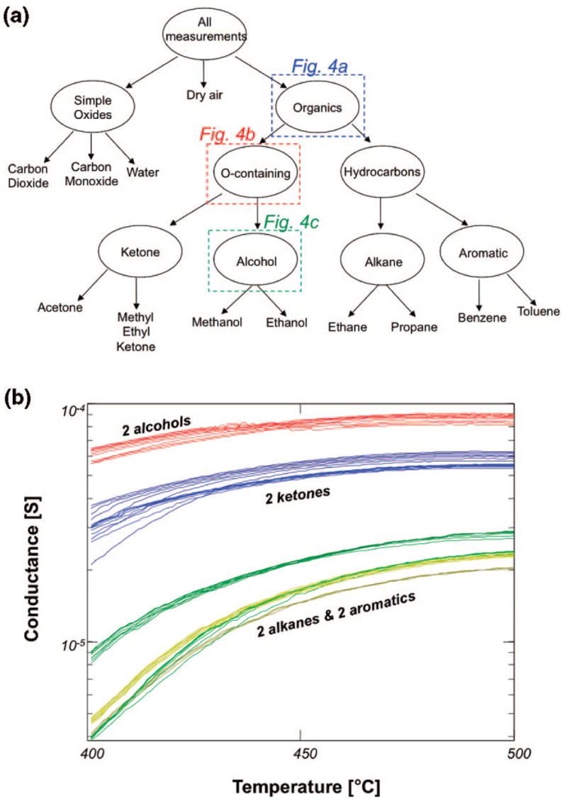
Divide-and-conquer approach to classification of the training data. (a) The hierarchy used to categorize the analytes present in the training data. (b) A region of raw data from sensor 1 with a similar conductance vs temperature profile for all four alkanes and aromatics, a separate profile for both ketones, and a third profile for both alcohols. Line color represents the analyte present during measurement, using the same color code as in Figure 2a. Though difficult to distinguish, between 7 and 10 overlapping lines of each color are plotted, representing repeated measurements. The presented data represent less than 2% of the overall microarray data set.

To resolve chemical identity, we begin with a simple event detection task that differentiates a nonevent (dry air) from two types of chemical events: presence of an organic or presence of a simple oxide. To perform this event detection task, we choose a subset of sensor features that provides maximum discrimination between samples of these three different categories and at the same time shows low variance across members within the same group. The feature selection is based on their modified t-statistic:²³

$$t=\frac{\mid {\mu }_i-{\mu }_j\mid }{{\sigma }_i+{\sigma }_j}$$ (2)

where μ_i and σ_i are the mean and standard deviation of all of the measurements from a particular sensor at a particular temperature within analytes of chemical class i, and μ_j and σ_j are the corresponding values within analytes of chemical class j. For each categorization problem within the divide-and-conquer approach, only those data features with maximal t-statistic were selected (for categorizations including more than two chemical classes, the average pairwise separability was used).

Using such a discrimination method, we found that species like benzene, which were difficult to detect using the all-at-once approaches (see Figure 2a), can be easily identified. In addition, each category has a large and diverse membership, which, as we will show later, allows generalization beyond the analytes of the training set. For building the subsequent levels of the hierarchy, the subcategories are further divided based upon more specific chemical features. Each time, only the training data collected within the analyte(s) belonging to that specific subcategory are used for categorization, excluding from consideration all of the data collected for other analytes. Within this reduced set of training data, the sensor features with maximal t-statistic for making the desired distinction are determined.

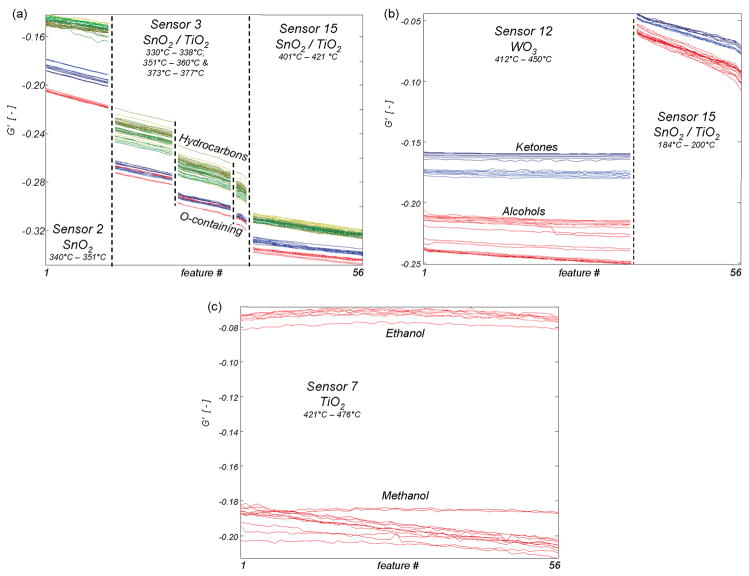
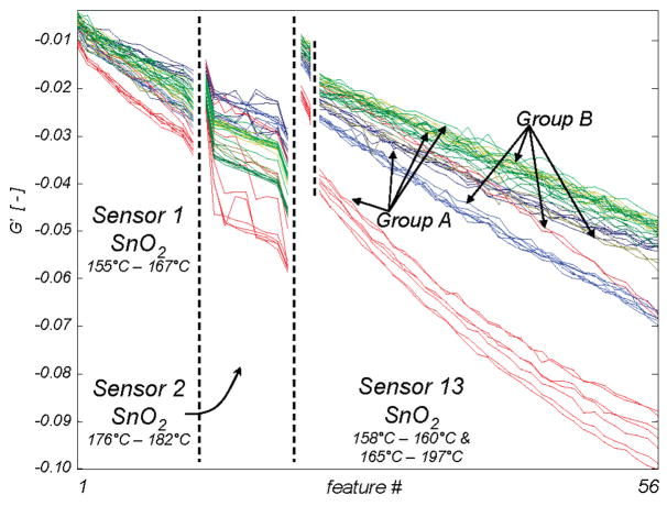
As an example, the 56 drift-corrected (G′) data points with maximal t-statistic, just 1% of the total collected, for grouping the organics into those that either do or do not contain oxygen are shown in Figure 4a; the best data points for grouping those that do contain oxygen into either alcohol or ketone are shown in Figure 4b; and, finally, the best data points for grouping the alcohols into either methanol or ethanol are shown in Figure 4c. Note that, for each discrimination level, the data from limited subsets of operating temperatures within a few select sensors are used. Supporting Information Figure S-5 shows the drift-corrected conductance data collected during the training phase for each sensor at each temperature and indicates, for each question in the hierarchy, whether that datum is used to answer that question.

Figure 4.

Drift-corrected raw data used for various categorization tasks. For each task, the data represent the 1% of data points with maximal t-statistic. Line color represents the analyte present during measurement, using the same color code as in Figure 2a. (a) Categorization of organics into those that do or do not contain oxygen. For simplicity, only data collected at 3 μmol/mol analyte concentrations are shown. (b) Categorization of oxygen-containing organics into alcohols or ketones. (c) Categorization of alcohols into methanol or ethanol.

The number of features selected for each question is an important parameter that affects the success of the technique. It is important to note that the distribution of t-statistics for sensor features critically depends on the complexity of the classification problem. Supporting Information Figure S-6 shows the distribution of t-statistics for each question in the hierarchy. For more general problems at higher levels of the hierarchy, the groupings of chemical species are rather loose. For example, the members of simple oxides group, CO, CO₂, and H₂O, do not have particularly similar chemistry. Hence, the probability of finding features that allow these chemicals to cluster together and at the same time distinguish them from the other organics group is low. On the other hand, for more specific discrimination tasks at the bottom levels of hierarchy (e.g., methanol vs ethanol), the class memberships are very well defined and therefore these individual analytes can be easily discriminated with very few optimal features. Thus, as detailed in Supporting Information, Table S-1, we have used in our approach more features for the initial questions and fewer features for later questions.

As a simplified strategy, we have also analyzed our data using a constant number of features across all levels of the hierarchy. By systematically varying the number of features selected, we find a peak performance level when using ≈10% of the total features for each step in the hierarchy. When using fewer than 10% of the features, we observed that there were many misclassifications for the very first task (simple oxide vs dry air vs organics). This was expected as the chemical groups at this level are not well defined compared to the lower levels and more features are required for addressing this problem. When using more than 10% of the features, the classification performance again dropped as less relevant features were included (especially at the lower levels). This is detailed in Supporting Information Figure S-7.

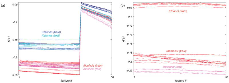
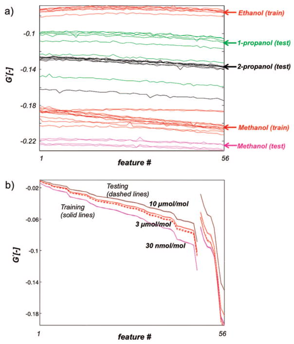
The multistep approach uses only those features that provide optimal separation between subsets of analytes. By limiting the analysis to sensor responses that are highly repeatable within an analyte group and that provide maximum discriminability between different analyte groups, robustness against drift is implicitly incorporated into the approach. Figure 5a shows the sensor features selected from the training data used for categorization of the alcohols versus ketones, as measured during the training and testing phases. Figure 5b shows the corresponding sensor features for categorization of ethanol versus methanol. Figure 5a shows the generalizability of this approach, and Figure 5b further demonstrates that reliable recognition of individual analytes is also possible. The stability in the sensor features selected from the training data using the modified t-statistic demonstrates how our feature selection approach mitigates drift, even if the overall sensor response profile has changed significantly.

Figure 5.

(a) Response of sensor–temperature features that were selected from the training data to discriminate alcohols from ketones. Both training and test measurements are shown. (b) Similar plot showing response of sensor–temperature features selected to discriminate ethanol from methanol (ethanol test data are not present because ethanol was not a member of the test set).

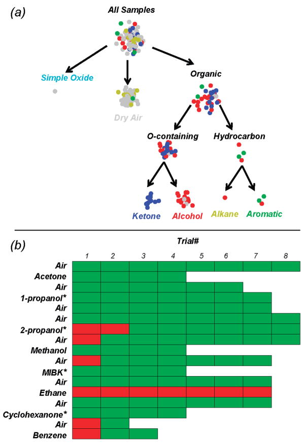
The drift-corrected data from the test phase, including the new analytes and those repeated from the training set, were categorized using the hierarchical scheme built from the training data. The data were classified using a k-nearest neighbor classifier²³ based on a Euclidean distance measure on the selected features (k = 3; k values of 1–9 exhibited nearly identical results). Figure 6a schematically shows the results, with dot color indicating the chemical group. Figure 6b shows the success or failure in classification of each measurement in the test phase. Other than ethane, the only misclassifications were during apparent lag times in recognition during the first one or two measurements after introduction or removal of some analytes. Unlike the training data, where introduction and removal of analytes were explicitly known, nothing was assumed of the test data. Thus, though in the training data the transitional measurements were manually removed, this was not done to the test data and is the likely cause of these transitional misclassifications. Ethane could not be distinguished from dry air during the test phase. It is likely that the sensors were not sufficiently sensitive to ethane, a relatively nonreactive molecule, to overcome the drift induced during the aging process. Despite these difficulties, the overall success rate in categorization of the test phase, including the new analytes and those repeated from the training phase, was 87%. The new alcohols and ketones were successfully categorized nearly every time.

Figure 6.

Hierarchical categorization of the test data. (a) Graphical view of the traversal of each measurement through the hierarchy. The chemical family of the analyte present during measurement is color-coded: gray, dry air; cyan, simple oxide; red, alcohol; blue, ketone; yellow, alkane; and green, aromatic (note that no simple oxides were used in the test phase). (b) Chart of the accuracy of placement of each measurement into its proper category: green box, correct placement; red, incorrect placement. Analytes not included during the training phase are indicated with an asterisk. The order of analyte exposure during the test phase is as shown, progressing from left to right and then top to bottom.

How might unknown analytes be handled in the scheme? In our evaluations, we stopped at the levels of determining the functional group of the test analytes. In Figure 7a, we add to Figure 5b the testing data collected when presenting the new alcohols. While the “training” and “testing” measurements of methanol are extremely close to each other in nearest-neighbor space, the two newer alcohols (1-propanol, 2-propanol) lie between the two known alcohols (methanol, ethanol) and, with some misclassifications, can be recognized as unknowns (i.e., the propanols would be classified as unknown alcohols, and not misidentified as methanol or ethanol) by setting a threshold on the distance measure.

Figure 7.

(a) Response of sensor–temperature features that were selected from the training data to discriminate ethanol from methanol. Both training and test measurements (including all three alcohols measured in the test phase: methanol, 1-propanol, and 2-propanol) are shown. (b) Response of sensor–temperature features that were selected from the training data to discriminate 30 nmol/mol methanol vs 3 μmol/mol methanol vs 10 μmol/mol methanol. Both training and test measurements (taken at 3 μmol/mol) are shown.

Similarly, how might different analyte concentrations be handled in the scheme? Concentration information may be obtained by adding to the hierarchy a final, lowest level for this purpose. Figure 7b shows sensor features selected from the training data used for categorization of the 30 nmol/mol methanol versus 3 μmol/mol methanol versus 10 μmol/mol methanol, as measured during the training (solid lines) and testing phases (dashed lines). The concentration during the testing phase was 3 μmol/mol methanol, and as can be seen, the test concentration is correctly identified. No normalization was necessary as both concentration-invariant and concentration-dependent features are available in the temperature spectra. The concentration-invariant features were used at higher levels and concentration-dependent features were used to quantify concentrations.

The ability to recognize pretrained or behaviorally important odors and to generalize to new odors based upon chemical similarity with known odorants are important challenges faced by both biological and artificial chemical sensing systems. Even though the analytical requirements of these tasks are at odds with each other, the biological system demonstrates an amazing ability to deal with these issues. What signal-processing strategy followed by the olfactory system allows it to address these analytical problems reliably? Physiological¹⁵ and behavioral²⁴ studies reveal that biological olfaction uses time as an additional coding dimension to decouple these tasks: initial coarse, generalizable representation gets refined over time by adding additional features that allow finer discrimination. This divide-and-conquer approach contrasts the conventional monolithic approaches followed in artificial olfaction where no distinction is made between the generalization and the recognition problems. While appropriate for highly orthogonal data, where analytes are ordered based upon their constituent chemical features,⁹ the performance of such approaches is significantly affected when dealing with sensor responses with low signal-to-noise ratios and high variability due to sensor aging (see Figure 2c). More importantly, these approaches lack the ability to examine the presence of a desired organization of the chemical space and therefore lack the flexibility to be tuned for a specific application.

We found that much of the success of the divide-and-conquer approach to mitigate errors due to drift was due to the following: (a) subdivision of the problem into a series of recognition tasks, each involving only a subset of analytes, and (b) independent selection of high signal-to-noise response features for each task. We observed that using all of the sensor response features for every question leads to a reduced overall successful classification rate of 31% for the test data (the great majority of the successes were dry air). Supporting Information, Figure S-8 shows the test data classification using the hierarchy without feature selection.

How flexible is the choice of groupings within the hierarchy? To examine whether discrimination between any two groups can be a subtask in the hierarchy, we designated two groups: A (ethanol, acetone, propane, toluene) and B (methanol, methyl ethyl ketone, ethane, benzene). These groupings were made such that there are no chemical features that distinguish one group from the other. Figure 8 shows that even the best features selected from the training data for these groupings show considerable spread within each group and no separation between the groups. This can be compared to Figure 4a, which is a more chemically logical categorization for the same set of analytes. This test implies that the data features selected during the more sensible categorizations relate to repeatable chemical interactions between the sensors and specific chemical features of the analytes. Furthermore, the ability to find these repeatable interactions for multiple levels of the hierarchy shows that chemical information at multiple levels of abstraction is available from the temperature spectra of metal oxide chemiresistors. Though it does not seem possible to use this technique to classify analytes according to arbitrary groupings, the use of alternate or multiple hierarchies is not precluded. For example, a carbon chain length-based scheme may be useful in classifying the analytes studied here.

Figure 8.

The 1% of drift corrected raw data points with maximal t-statistic for categorization of the organics into group A (ethanol, acetone, propane, toluene) or B (methanol, methyl ethyl ketone, ethane, benzene). Line color represents the analyte present during measurement, using the same color code as in Figure 2a.

CONCLUSIONS

In this work, we have shown that chemical sensors can be used within a biologically inspired, hierarchical categorization scheme to provide a reliable, highly drift-resistant mechanism for useful classification of both previously trained chemicals and those never seen before. This ability is possible because of the discovery that temperature-controlled, semiconductor chemical sensors are responsive to multiple levels of chemical information. The methodology developed is robust against drift in the signal, since it relies upon finding where analyte–sensor chemical interactions occur with high consistency. The method does not rely upon complex and delicate mathematical formulations that can overfit the training data. Key aspects to the approach are an analytically rich database, a sensible hierarchy scheme, and a selection method to determine which data are most useful for a particular categorization. Temperature-modulated sensor arrays built on MEMS microhotplates were found to be an excellent platform, although not uniquely so, with which to accomplish this task. The methods described may enable the use of chemical sensor arrays as miniature, inexpensive analytical tools.

Supplementary Material

Supplementary

SUPPORTING INFORMATION AVAILABLE

Additional information as noted in text. This material is available free of charge via the Internet at http://pubs.acs.org.

References

- 1.Freund MS, Lewis NS. Proc Natl Acad Sci U S A. 1995;92:2652–2656. doi: 10.1073/pnas.92.7.2652. [DOI] [PMC free article] [PubMed] [Google Scholar]
- 2.Dickinson TA, White J, Kauer JS, Walt DR. Nature. 1996;382:697–700. doi: 10.1038/382697a0. [DOI] [PubMed] [Google Scholar]
- 3.Persaud K, Dodd G. Nature. 1982;299:352–355. doi: 10.1038/299352a0. [DOI] [PubMed] [Google Scholar]
- 4.Albert KJ, Lewis N, Schauer C, Sotzing GA, Stitzel SE, Vaid TP, Walt DR. Chem Rev. 2000;100:2595–2626. doi: 10.1021/cr980102w. [DOI] [PubMed] [Google Scholar]
- 5.Nagle TH, Schiffman SS, Gutierrez-Osuna R. IEEE Spectrum. 1998;35:22–34. [Google Scholar]
- 6.Shevade AV, Homer ML, Taylor CJ, Zhou HY, Jewell AD, Manatt KS, Kisor AK, Yen SPS, Ryan MA. J Electrochem Soc. 2006;153:H209–H216. [Google Scholar]
- 7.Jurs PC, Bakken GA, McClelland HE. Chem Rev. 2000;100:2649–2678. doi: 10.1021/cr9800964. [DOI] [PubMed] [Google Scholar]
- 8.Gutierrez-Osuna R. IEEE Sens J. 2002;2:189–202. [Google Scholar]
- 9.Sisk BC, Lewis NS. Sens Actuators, B: Chem. 2003;96:268–282. [Google Scholar]
- 10.Grate JW, Patrash SJ, Kaganove SN, Abraham MH, Wise BM, Gallagher NB. Anal Chem. 2001;73:5247–5259. doi: 10.1021/ac010490t. [DOI] [PubMed] [Google Scholar]
- 11.Boger Z, Meier DC, Cavicchi RE, Semancik S. Sens Lett. 2003;1:86–92. [Google Scholar]
- 12.Holmberg M. Handbook of Machine Olfaction. 1. Wiley-VCH; Weinheim: 2002. [Google Scholar]
- 13.Ngai J, Chess A, Dowling MM, ecles N, Macagno ER, Axel R. Cell. 1993;72:667–680. doi: 10.1016/0092-8674(93)90396-8. [DOI] [PubMed] [Google Scholar]
- 14.Hallem E, Carlson JR. Cell. 2006;125:143–160. doi: 10.1016/j.cell.2006.01.050. [DOI] [PubMed] [Google Scholar]
- 15.Friedrich RW, Laurent G. Science. 2001;291:889–894. doi: 10.1126/science.291.5505.889. [DOI] [PubMed] [Google Scholar]
- 16.Raman B, Sun PA, Gutierrez-Galvez A, Gutierrez-Osuna R. IEEE Trans Neural Netw. 2006;17:1015–1024. doi: 10.1109/TNN.2006.875975. [DOI] [PubMed] [Google Scholar]
- 17.Meier DC, Taylor CJ, Cavicchi RE, White E, Semancik S, Ellzy MW, Sumpter KB. IEEE Sens J. 2005;5:712–725. [Google Scholar]
- 18.Semancik S, Cavicchi RE, Wheeler MC, Tiffany JE, Poirier GE, Walton RM, Suehle JS, Panchapakesan B, Devoe DL. Sens Actuators, B. 2001;77:579–591. [Google Scholar]
- 19.Semancik S, Cavicchi R. Acc Chem Res. 1998;31:279–287. [Google Scholar]
- 20.Hines EL, Boilot P, Gardner JW, Gongora MA. In: Handbook of Machine Olfaction. Pearce TC, Schiffman SS, Nagle TH, Gardner JW, editors. Wiley-VCH: Weinheim; 2002. pp. 133–160. [Google Scholar]
- 21.Bermak A, Belhouari S, Shi M, Martinez D. In: The Encyclopedia of Sensors. Grimes CA, Dickey EC, Pishko MV, editors. Vol. 7. American Scientific Publishers; Stevenson Ranch, CA: 2006. pp. 349–365. [Google Scholar]
- 22.Zhang C, Suslick KS. J Agric Food Chem. 2007;55:237–242. doi: 10.1021/jf0624695. [DOI] [PubMed] [Google Scholar]
- 23.Duda RO, Hart PE, Stork DG. Pattern Classification. 2. Wiley-Interscience; New York: 2000. [Google Scholar]
- 24.Rinberg D, Koulakov A, Gelperin A. Neuron. 2006;51:351–358. doi: 10.1016/j.neuron.2006.07.013. [DOI] [PubMed] [Google Scholar]
Associated Data
This section collects any data citations, data availability statements, or supplementary materials included in this article.
Supplementary Materials