Optimized theory for simple and molecular fluids

Abstract

An optimized closure approximation for both simple and molecular fluids is presented. A smooth interpolation between Perkus-Yevick and hypernetted chain closures is optimized by minimizing the free energy self-consistently with respect to the interpolation parameter(s). The molecular version is derived from a refinement of the method for simple fluids. In doing so, a method is proposed which appropriately couples an optimized closure with the variant of the diagrammatically proper integral equation recently introduced by this laboratory [K. M. Dyer et al., J. Chem. Phys. 123, 204512 (2005)]. The simplicity of the expressions involved in this proposed theory has allowed the authors to obtain an analytic expression for the approximate excess chemical potential. This is shown to be an efficient tool to estimate, from first principles, the numerical value of the interpolation parameters defining the aforementioned closure. As a preliminary test, representative models for simple fluids and homonuclear diatomic Lennard-Jones fluids were analyzed, obtaining site-site correlation functions in excellent agreement with simulation data.

I. INTRODUCTION

Within the theory of simple liquids, the problem of obtaining a suitable and accurate description of relevant physical quantities has been well studied in the literature.^1-5 Among the different methods proposed to tackle this problem, integral equation (IE) theory has been useful due to the precision reached in its predictions and its low computational cost.⁶ Indeed, IE's represent a valuable tool for computing approximate pair-distribution functions, g(r), from which it is possible to obtain the thermodynamic properties of interacting fluid systems. These theories are traditionally formulated by providing a set of two equations, namely, the integral equation which defines a direct correlation function c(r) in terms of g(r) and a closure relationship involving an additional functional B(r)=B[g(r)] called a bridge function. To be robust, these techniques require an accurate knowledge of B(r). Within an exact framework, namely, the graphical expansions, bridge functions are unambiguously defined. However, such expansions for B(r) in powers of the density involve an infinite sum of highly connected diagrams preventing a simple computation of the multidimensional integrals and so cannot be fully utilized in practice.

In the case of simple fluids, this led, during the last half century, to a number of different approximations which were good for different particular applications depending on state point and potential energy function, such as the Perkus-Yevick (PY),^7,8 hypernetted chain (HNC),^9,10 and mean spherical approximation (MSA).¹¹ These approximations belong to the small group of closures which could be derived from simple arguments, either by using Percus' functional expansion^7,12,13 or by summing specific infinite subset of terms or diagrams.^9,14 Beyond providing good qualitative behavior these approximations have not produced uniformly good quantitative results in general.¹ Further, these approaches, in general, generate thermodynamic inconsistency, e.g., a nonequivalence between different routes to thermodynamics. This has encouraged refined approximations to overcome those difficulties.^15-28 Such is the case of hybrid theories which mix two of the approximations via a switching function. Further direct calculation of a series of bridge diagrams leads to considerable improvement in the results but dramatically increases the computational complexity.^29,30

Notwithstanding the success of IE's to qualitatively describe the structure of simple one-component systems, considerable work is still devoted to derive improved approximations which accurately describe the thermodynamics of molecular fluids. There are two main forms which integral equations commonly take for molecular fluids.^1-3 The interaction site formalism developed by Chandler and co-workers^31-35 is designed to utilize intermolecular interactions in terms of spherically symmetric site interactions and site-site inter- and intramolecular correlations. Such is the case of the reference interaction site model (RISM) theory^5,31 and its generalization^36,37 which have been applied to nonpolar and strongly polar molecular fluids, respectively. Beyond obtaining a qualitative description of such systems, inconsistencies and quantitative limitations in the description of the short and long range structures were found.³⁸ A more sophisticated approximate theory was introduced by Chandler, Silbey, and Ladanyi³⁹ (CSL) which appropriately constructed the correlation functions by splitting contributions in four subclasses of terms in such a way that certain inconsistencies presented in RISM theory were removed. Rossky and Chiles⁴⁰ complemented the proper interaction site model (PISM) theory by providing HNC-like closure relationships for each subclass of correlations giving the possibility of exploring a wide variety of approximations borrowed from atomic fluids. Unfortunately, the obtained numerical results did not yield a practical improvement over RISM theory.

Lupkowski and Monson⁴¹ developed a cluster perturbation based on CSL equations. That formalism was successfully tested on some simple models. Its extension to more complex systems is nontrivial, however, mainly because of the limited amount of information available about the structure and thermodynamics of the reference system.

A more complete analysis is required to apply PISM theories to more complex molecular fluids such as water.^42,43 It is well known that the structure and thermodynamics of simple liquids are mainly governed by short-ranged repulsive interactions between molecules, the molecular structure of water is strongly affected by the presence of charges and of the corresponding molecular anisotropy where neither PY nor HNC closures closely reproduce simulation data.⁴² One could then consider either improving the integral equation or the closures, in particular, studying the selected properties of various bridge functions.^29,30,43

Recently, this laboratory^44,45 has reanalyzed the diagrammatically proper theory. A different integral equation having a density matrix with nondiagonal elements containing screened densities was proposed. By computing the correction to first order and using a HNC closure, the theory was tested on homonuclear diatomic fluids obtaining a significant improvement in the prediction of site-site correlation functions over PISM-HNC theory.

Following that work, the purpose of this paper centers on developing a new closure approximation which self-consistently provides a more accurate description of molecular fluids. In doing so, we begin our approach in Sec. II by presenting an optimizable closure approximation in the spirit of Stell.¹³ To obtain the expression for the closure we have utilized Percus' functional expansion to first order in the density of a functional which depends on both density and activity in a fictitious field and a free parameter which is determined by first principles, e.g., minimizing the excess chemical potential. In this way thermodynamic optimization is achieved as first suggested by Stell some years ago.¹³ In Sec. III, our approximation is compared with simulation results over a range of thermodynamic states. We first test simple fluids for the LJ potential at several densities and temperatures. The following section is involved with the extension to the molecular fluids. We have divided the correlation functions present in our new closure in four subclasses to get the four “proper” closures. We tested our approximation for homonuclear diatomic fluids at several state points. These results are presented in Sec. V, leaving our conclusions for the last section.

II. SIMPLE FLUIDS

A. Optimized closure approximation

The formally exact closure relationship for simple fluids, derived from graphical expansions, is expressed by the following formula:¹⁴

$$g\left(r\right)=\exp [-\beta u\left(r\right)+t\left(r\right)+B\left(r\right)],$$ (1)

where t(r)=h(r)−c(r) is the indirect correlation function, h(r)=g(r)−1 the total correlation function, B(r) the bridge function, β=1/k_BT, where k_B the Boltzmann constant and T the absolute temperature, and u(r) the pair potential. To obtain good predictions of pair-correlation functions for dense fluids we need an accurate approximation for B(r). Lacking this in general, we follow the well-known Percus' generating functional expansion^7,12 because it allows systematic derivation of different approximate expressions to relationship (1) by a unified method. In fact, this technique allows one to establish how various functionals, depending on the thermodynamics of an initially homogeneous fluid, change due to a perturbation generated by an external, even fictitious field on a particle fixed at the origin.¹³ For example, the variation to first order with respect to the difference between the local density and the average density Δρ=ρ(r)−ρ of the functional of density and activity F_PY[ρ(r),z(r)]=ρ(r)/z(r) yields the well-known PY closure approximation

$$g\left(r\right)\simeq \exp [-\beta u\left(r\right)+\ln [t\left(r\right)+1]],$$ (2)

which may be interpreted as having a bridge function of the form B_PY(r)=−t(r)+ln[t(r)+1]. In the same way, the functional F_HNC[ρ(r),z(r)]=ln[ρ(r)/z(r)] leads to the HNC closure approximation

$$g\left(r\right)\simeq \exp [-\beta u\left(r\right)+t\left(r\right)],$$ (3)

where now the bridge function B_HNC(r) is equal to zero. Given that the PY approximation (2) can be obtained by linearizing the HNC relationship (3) with respect to t(r), these closures display relationships. This is a direct consequence of the relationship between their corresponding generating functionals, namely, F_HNC=ln[F_PY].

This leads us to consider the following parametric generating functional:

$$F_I=\ln \left[a_1\frac{\rho \left(r\right)}{z\left(r\right)}+a_2\right],$$ (4)

where parameters a₁ and a₂ are introduced in such a way that we recover F_HNC and F_PY closures by assigning specific values to these parameters. Indeed, the resulting variational calculation with F_I yields the following “interpolating” closure approximation:

$$g\left(r\right)\simeq \exp [-\beta u\left(r\right)]\left\{-a+(a+1)\exp \left[\frac{t\left(r\right)}{a+1}\right]\right\},$$ (5)

where a single parameter a=a₂/a₁ is used. Thus, we recover expressions (2) and (3) for a→∞ and a=0, respectively. In between, a smooth transition is obtained, generating a family of closure approximations. The corresponding expression for the bridge function that interpolates from that appropriate to HNC, B_HNC=0, to the PY bridge approximation from HNC, B_PY, becomes

$$B_I\left(r\right)=-t\left(r\right)+\ln \left[-a+(a+1)\exp \left[\frac{t\left(r\right)}{a+1}\right]\right],$$ (6)

which, as many other closure approximations,^{7,15,19-21,23-26} is a functional of t(r) rather than the rigorously expected g(r). In the next subsection, we analyze the consequences deriving from this.

Expression (6) recovers the physical interpretation of the functions B_PY and B_HNC. Recall that B_PY(r) can be formally obtained by approximating an infinite subset of bridge diagrams in which one judiciously replaces certain f bonds of the diagrams by −1. This is based on the fact that the high connectivity of these diagrams makes the integrals dominated by regions where field points are close together. On the other hand, if one replaces the f bonds in those diagrams by zero, one recovers B_HNC(r). These results can also be obtained from Eq. (6), representing an intermediate approximation for the f bonds which go from zero to −1 when the parameter a is going from zero to infinity. Indeed, this can be explicitly seen by expanding Eq. (6) in powers of t(r),

$$B_I\left(r\right)\simeq -\frac{t{\left(r\right)}^2}{2}{b}_1\left(a\right)+\frac{t{\left(r\right)}^3}{3}{b}_2\left(a\right)-+\cdots ,$$ (7)

and afterward comparing with the PY approximation

$$B_{\mathrm{PY}}\left(r\right)\simeq -\frac{t{\left(r\right)}^2}{2}+\frac{t{\left(r\right)}^3}{3}-+\cdots ,$$ (8)

where b₁(a)=1−1/(a+1), b₂(a)=1−(1+3a/2)/(a+1)². It is clear that b_i(a)→1 for a→∞ and b_i(a)→0 for a→0.

In the next subsection we present a robust numerical technique to determine the optimal value for this parameter from first principles.

B. Approximate expression for the chemical potential

The well-known Kirkwood formula,⁴⁶ utilized for obtaining analytic expressions for the excess chemical potential μ_ex, reads

$$\beta {\mu }_{\mathrm{ex}}\equiv \rho {\int }_0^{1}d\lambda \int d\mathbf{r}\frac{\partial \beta u(r,\lambda )}{\partial \lambda }g(r,\lambda ),$$ (9)

where the parameter λ couples the interactions of a single atom, referred to as the solute or test particle, to the rest of the atoms in the fluid, or solvent, with ρ the density of the solvent.

The λ integral can be carried out following the useful route developed by Morita and Hiroike⁴⁷ in which an expression for ∂βu(r,λ)/∂λ is obtained by differentiating the exact closure [Eq. (1)] with respect to λ and substituted into Eq. (9). Further, the correlation functions are assumed to be linearly dependent on λ,⁴⁸ e.g., h(r,λ)≃λh(r) and c(r,λ)≃λc(r), obtaining

$$\begin{array}{cc}\hfill \beta {\mu }_{\mathrm{ex}}=& \rho \int d\mathbf{r}[\frac{h{\left(r\right)}^2}{2}-c\left(r\right)+B\left(r\right)-\frac{h\left(r\right)c\left(r\right)}{2}\phantom{]}\hfill \\ \hfill & \phantom{[}+h\left(r\right)\left(B\left(r\right)-{\int }_0^{1}d\lambda B(r,\lambda )\right)].\hfill \end{array}$$ (10)

Our assumption that the bridge function is expressible uniquely as a function of t(r), e.g., B(r)=B_I(t(r)), introduces a possible path dependence into the results of the interpretation over λ.^48-50 We find that a useful expression for the excess chemical potential is given by the following approximate formula:

$$\beta {\mu }_{\mathrm{ex}}\left(a\right)\simeq -\rho \int d\mathbf{r}\{h\left(r\right)-t\left(r\right)ℐ[t\left(r\right),h\left(r\right),a]\},$$ (11)

where

$$ℐ=\frac{\{[h\left(r\right)+1]\ln [y\left(r\right)∕a]+\ln \left[a\right]+[h\left(r\right)(a+1)∕t\left(r\right)]\mathrm{Re}[{\mathrm{li}}_2(y\left(r\right)∕a+1)-{\mathrm{li}}_2((a+1)∕a)]\}}{t\left(r\right)},$$ (12)

li₂(x) being the well-known dilogarithm function⁵¹ and y(r)=−a+(a+1)exp[t(r)/(a+1)].

For testing proposes, we have explicitly computed this expression on a number of examples with the exact results coming from Morita and Hiroike. In fact, for approximate closures near to HNC we recover the exact value as expected. Otherwise, we obtain a small difference but the shape of the curves is in very good agreement. Given that we are interested in determining the numerical value of the parameter a which minimizes the chemical potential, both expressions provide a very similar derivative. From the numerical point of view, this represents a significant advantage since this gives a more efficient way of computing the excess chemical potential than explicit quadrature of Eq. (9). This allows us to perform an optimization in which a systematic evaluation of the chemical potential is required. Expression (11) can be viewed as an objective function with which to predict the value of the parameter a.

The outline of the algorithm used to solve the problem can be summarized by the following steps:

• (1) Guess initial values for the unknown a parameter(s).

• (2) Solve equations by using standard iterational or variational routines.

• (3) Use the corresponding correlation functions to compute the chemical potential.

• (4) Use a suitable (multidimensional) minimization routine (e.g., steepest decent, powell, simplex, etc.) to generate new estimates of the a parameter(s).

• (5) Repeat steps 2–4 to obtain the convergence for the value(s) of the parameter(s).

In addition, it will be certainly instructive to analyze the advantages and limitations of this optimizing process in predicting thermodynamic quantities for atomic fluids. In the next section, we have analyzed the Lennard-Jones (LJ) fluid at several thermodynamic states, where efficiency and accuracy have been quantitatively tested against molecular dynamics (MD) simulation.

III. APPLICATION TO ATOMIC FLUIDS

This optimized approximate theory for simple fluids contains three elements: a new closure approximation given by formula (5) with the corresponding expression for the bridge function (6), the OZ integral equation,⁵³ and an approximate analytic expression for the excess chemical potential [Eq. (11)].

It is well known that thermodynamically consistent or optimized approaches like this one lead to correlation functions and thermodynamic properties which can produce excellent agreement with simulation data. Such is the case of Rogers and Young's method²⁴ (RY) which was successfully applied to repulsive inverse power potentials including hard spheres and the one-component plasma. Note that we can recover the RY results by replacing the constant 1/(1+a) in Eq. (5) by the switching function f(r)=1−exp(−αr). In addition, this kind of approach is easily generalized to the case of mixtures as has been explicitly shown for binary mixtures.⁵² In considering the thermodynamics, the success of these approaches is largely due to the fact that for purely repulsive potentials there are regions of the phase diagram where PY and HNC bracket the simulated pressure and densities. In such a case, one achieves thermodynamic self-consistency.

The previous analysis is different for potentials which also include an attractive interaction. In particular, for LJ interactions the simulation result is not bracketed, with PY lying closer than HNC.¹ We find that when bracketing occurs the value of a moves toward the simulated value and where PY is closest a yields PY. This behavior demonstrates another benefit of our optimized closure approach.

Figures 1 and 2 show the comparison between the site-site correlation function g(r) obtained from the numerical solution of our equations (solid lines) and simulation (symbols). Specifically, Fig. 1 shows the results for the simple LJ fluid at fixed reduced temperature T* ≡ 1/(βε)=2.74 and reduced densities ρ* ≡ ρσ³=0.9 (circles) and 0.5 (squares), where ε is the depth of the attractive interaction and σ characterizes the width of the repulsive core. Figure 2 shows the results corresponding to fixed reduced density ρ*=0.5 and reduced temperatures T*=1.35 (circles) and 1.827 (squares). In all of these cases, our predictions correspond to our closure approximation evaluated with the parameter a≃1000, where the free energy function is quite flat and optimization can be terminated.

FIG. 1.

Simple LJ fluid: correlation function g(r) at reduced temperature T*=2.74. Circles and squared symbols correspond to simulation data at reduced densities ρ*=0.9 and 0.5, respectively. Solid lines represent our predictions.

FIG. 2.

Simple LJ fluid: correlation function g(r) at reduced density ρ*=0.5. Circles and squared symbols correspond to simulation data at reduced temperatures T*=1.35 and 1.827, respectively. Solid lines represent our predictions. T*=1.827 is vertically shifted.

All of these results show that our predictions are in good agreement with simulation. In particular, we observe the expected PY match in the location of the peaks corresponding to the first four neighbor solvation shells. For each tested thermodynamic state, we have also explicitly compared predictions coming from evaluating closure approximation (5) at different values of the parameter a, adjusting the parameter to best fit simulation on the range of distances between the first and the third peaks. As expected, the best match is obtained by that value of the parameter a which minimizes the excess chemical potential. We did not find significant differences in predictions obtained from the correlation function for values of the parameter a larger than 100. In other words, this value can be considered as that which essentially reproduces the PY closure approximation limit.

Finally, it is worth mentioning that members of this class of interpolating closures, such as the one developed by Zerah and Hansen,¹⁵ achieve thermodynamic consistency in LJ fluids by basically partitioning the potential into a repulsive reference part and an attractive part obtaining an interpolating closure between the HNC and MSA approximations. Unfortunately, the extension of this kind of approaches to diagrammatically proper integral equations for molecular fluids is nontrivial. On the other hand, and as it shall be shown in the next section, the aforementioned thermodynamic consistency for molecular fluids can be recovered by using a parametrization of the appropriate bridge functions.

IV. EXTENSION TO MOLECULAR FLUIDS

In the previous sections, we presented a new closure approximation for simple fluids which was shown to provide results in good agreement with simulation as had previous approximations.^15,17 We now show how to use the approach to develop a useful approximate molecular theory based on the diagrammatically proper integral equation theory. Following Rossky and Chiles,⁴⁰ we begin by introducing a multicomponent version of our approximation (5) as follows:

$$g_{\alpha \gamma }\left(r\right)\simeq -{\mathit{ae}}^{-\beta u_{\alpha \gamma }\left(r\right)}+(1+a)e^{[-\beta u_{\alpha \gamma }\left(r\right)+t_{\alpha \gamma }\left(r\right)∕(1+a)]}.$$ (13)

Next, we divide the interaction site correlations term by term into the standard four graphical subclasses, depending whether or not either or both of the two labeled white circles (root points) associated with a graph are intersected by an s bond. The groups are: o (none), r (right), ℓ (left), and b (both). In this way, site-site pair-correlation functions in a molecular fluids are given by the sum of the four components, namely, $t_{\alpha \gamma }\left(r\right)=t_{\alpha \gamma }^o\left(r\right)+t_{\alpha \gamma }^r\left(r\right)+t_{\alpha \gamma }^{\ell }\left(r\right)+t_{\alpha \gamma }^b\left(r\right)=h_{\alpha \gamma }^o\left(r\right)-c_{\alpha \gamma }^o\left(r\right)+h_{\alpha \gamma }^r\left(r\right)-c_{\alpha \gamma }^r\left(r\right)+h_{\alpha \gamma }^{\ell }\left(r\right)-c_{\alpha \gamma }^{\ell }\left(r\right)+h_{\alpha \gamma }^b\left(r\right)-c_{\alpha \gamma }^b\left(r\right)$ and so on. Replacing these expressions into Eq. (13) after Rossky and Chiles, we arrive at the following closure approximation:

$$\begin{array}{cc}\hfill c_{\alpha \gamma }^o\left(r\right)=& -{\mathit{ae}}^{-\beta u_{\alpha \gamma }\left(r\right)}+(1+a)e^{[-\beta u_{\alpha \gamma }\left(r\right)+t_{\alpha \gamma }^o\left(r\right)∕(1+a)]}-1\hfill \\ \hfill & -t_{\alpha \gamma }^o\left(r\right),\hfill \\ \hfill c_{\alpha \gamma }^r\left(r\right)=& t_{\alpha \gamma }^r\left(r\right)e^{[-\beta u_{\alpha \gamma }\left(r\right)+t_{\alpha \gamma }^o\left(r\right)∕(1+a)]}-t_{\alpha \gamma }^r\left(r\right),\hfill \\ \hfill c_{\alpha \gamma }^{\ell }\left(r\right)=& t_{\alpha \gamma }^{\ell }\left(r\right)e^{[-\beta u_{\alpha \gamma }\left(r\right)+t_{\alpha \gamma }^o\left(r\right)∕(1+a)]}-t_{\alpha \gamma }^{\ell }\left(r\right),\hfill \\ \hfill c_{\alpha \gamma }^b\left(r\right)=& \left[t_{\alpha \gamma }^b\left(r\right)+\frac{t_{\alpha \gamma }^{\ell }\left(r\right)t_{\alpha \gamma }^r\left(r\right)}{1+a}\right]e^{[-\beta u_{\alpha \gamma }\left(r\right)+t_{\alpha \gamma }^o\left(r\right)∕(1+a)]}\hfill \\ \hfill & -t_{\alpha \gamma }^b\left(r\right).\hfill \end{array}$$ (14)

Observe that this closure becomes PISM-HNC and PISM-PY approximations for a→0 and a→∞, respectively, in such a way that expressions (14) can be seem to be the simplest generalization of our approximation (13) for proper site-site molecular fluids.

We can use this closure approximation in addition to the integral equation theory introduced earlier⁴⁵ in which the density matrix is shown to contain screened contributions. We extend our approach to include a separate variational parameter for each subclass following the splitting of the indirect correlations in our closure approximation (13),

$$\frac{t_{\alpha \gamma }\left(r\right)}{(1+a)}\to \frac{t_{\alpha \gamma }^o\left(r\right)}{(1+a^o)}+\frac{t_{\alpha \gamma }^r\left(r\right)}{(1+a^r)}+\frac{t_{\alpha \gamma }^{\ell }\left(r\right)}{(1+a^{\ell })}+\frac{t_{\alpha \gamma }^b\left(r\right)}{(1+a^b)}.$$

The closure must be constrained by two additional assumptions in order to preserve essential features of the theory. Specifically, the physical symmetry between r and ℓ elements is recovered by requiring a^r=a^l. Next, in the absence of intramolecular correlations, only the o elements are nonzero and the closure for $c_{\alpha \gamma }^o\left(r\right)$ should be that for the atomic case. This is achieved by assuming that the parameter a equals a^o. After taking this into account, our proposal for a closure approximation reads

$$\begin{array}{cc}\hfill c_{\alpha \gamma }^o\left(r\right)=& -a^o{e}^{-\beta u_{\alpha \gamma }\left(r\right)}+(1+a^o)e^{[-\beta u_{\alpha \gamma }\left(r\right)+t_{\alpha \gamma }^o\left(r\right)∕(1+a^o)]}-1\hfill \\ \hfill & -t_{\alpha \gamma }^o\left(r\right),\hfill \\ \hfill c_{\alpha \gamma }^r\left(r\right)=& \frac{(1+a^o)}{(1+a^r)}{t}_{\alpha \gamma }^r\left(r\right)e^{[-\beta u_{\alpha \gamma }\left(r\right)+t_{\alpha \gamma }^o\left(r\right)∕(1+a^o)]}-t_{\alpha \gamma }^r\left(r\right),\hfill \\ \hfill c_{\alpha \gamma }^{\ell }\left(r\right)=& \frac{(1+a^o)}{(1+a^r)}{t}_{\alpha \gamma }^{\ell }\left(r\right)e^{[-\beta u_{\alpha \gamma }\left(r\right)+t_{\alpha \gamma }^o\left(r\right)∕(1+a^o)]}-t_{\alpha \gamma }^{\ell }\left(r\right),\hfill \\ \hfill c_{\alpha \gamma }^b\left(r\right)=& (1+a^o)[\frac{t_{\alpha \gamma }^b\left(r\right)}{(1+a^b)}\phantom{]}\hfill \\ \hfill & \phantom{[}+\frac{t_{\alpha \gamma }^r\left(r\right)t_{\alpha \gamma }^{\ell }\left(r\right)}{{(1+a^r)}^2}]e^{[-\beta u_{\alpha \gamma }\left(r\right)+t_{\alpha \gamma }^o\left(r\right)∕(1+a^o)]}-t_{\alpha \gamma }^b\left(r\right).\hfill \end{array}$$ (15)

Note that this closure, depending on three parameters, becomes the previous one for a^o=a^r=a^b=a in such a way that expressions (15) can be considered to be a generalization of our approximation (13) for molecular fluids.

After rewriting Eqs. (15) suitably, we get the following expressions for the interpolating bridge functions:

$$\begin{array}{cc}\hfill b_{\alpha \gamma }^o\left(r\right)=& -t_{\alpha \gamma }^o\left(r\right)+\ln [-a^o+(1+a^o)e^{[t_{\alpha \gamma }^o\left(r\right)∕(1+a^o)]}],\hfill \\ \hfill b_{\alpha \gamma }^r\left(r\right)=& \frac{t_{\alpha \gamma }^r\left(r\right)}{(1+a^r)}[a^o{e}^{[-t_{\alpha \gamma }^o\left(r\right)-b_{\alpha \gamma }^o\left(r\right)]}-a^r],\hfill \\ \hfill b_{\alpha \gamma }^{\ell }\left(r\right)=& \frac{t_{\alpha \gamma }^{\ell }\left(r\right)}{(1+a^r)}[a^o{e}^{[-t_{\alpha \gamma }^o\left(r\right)-b_{\alpha \gamma }^o\left(r\right)]}-a^r],\hfill \\ \hfill b_{\alpha \gamma }^b\left(r\right)=& [a^o{e}^{[-t_{\alpha \gamma }^o\left(r\right)-b_{\alpha \gamma }^o\left(r\right)]}+1]\left[\frac{t_{\alpha \gamma }^b\left(r\right)}{(1+a^b)}+\frac{t_{\alpha \gamma }^r\left(r\right)t_{\alpha \gamma }^{\ell }\left(r\right)}{{(1+a^r)}^2}\right]\hfill \\ \hfill & -[t_{\alpha \gamma }^r\left(r\right)+b_{\alpha \gamma }^r\left(r\right)][t_{\alpha \gamma }^{\ell }\left(r\right)+b_{\alpha \gamma }^{\ell }\left(r\right)]-t_{\alpha \gamma }^b\left(r\right).\hfill \end{array}$$ (16)

As it will show in the next section, the simplicity of these expressions allows us to extend the previous approach developed for simple fluids to obtain an analytic, approximate expression for the molecular chemical potential. The resulting formula is then utilized for determining the three-unknown parameters of the theory by optimization.

A. Approximate expression for the molecular chemical potential

Lue and Blankschtein⁵⁴ have used proper integral equations for interaction site fluids to obtain a molecular version of the general expression [Eq. (10)] given for the excess chemical potential. In fact, they followed the same path as we did in Sec. II of the present article to obtain

$$\beta {\mu }_{\mathrm{ex}}\equiv \rho \underset{\alpha \gamma }{\Sigma }{\int }_0^{1}d\lambda \int d\mathbf{r}\frac{\partial \beta u_{\alpha \gamma }(r,\lambda )}{\partial \lambda }{g}_{\alpha \gamma }(r,\lambda ),$$ (17)

$$\begin{array}{cc}\hfill =& -\rho \underset{\alpha \gamma }{\Sigma }\int d\mathbf{r}\{\frac{\partial h_{\alpha \gamma }(r,\lambda )}{\partial \lambda }-(1+h_{\alpha \gamma }(r,\lambda ))\frac{\partial w_{\alpha \gamma }^o(r,\lambda )}{\partial \lambda }\phantom{\}}\hfill \\ \hfill & -(1+h_{\alpha \gamma }^o(r,\lambda )+h_{\alpha \gamma }^r(r,\lambda ))\times \frac{\partial w_{\alpha \gamma }^{\ell }(r,\lambda )}{\partial \lambda }\hfill \\ \hfill & -(1+h_{\alpha \gamma }^o(r,\lambda )+h_{\alpha \gamma }^{\ell }(r,\lambda ))\frac{\partial w_{\alpha \gamma }^r(r,\lambda )}{\partial \lambda }\hfill \\ \hfill & \phantom{\{}-(1+h_{\alpha \gamma }^o(r,\lambda ))\frac{\partial w_{\alpha \gamma }^b(r,\lambda )}{\partial \lambda }\},\hfill \end{array}$$ (18)

where

$$\begin{array}{cc}\hfill h_{\alpha \gamma }(r,\lambda )=& \underset{i=o,r,\ell ,b}{\Sigma }{h}_{\alpha \gamma }^i(r,\lambda ),w_{\alpha \gamma }^{o,r,\ell ,b}(r,\lambda )=t_{\alpha \gamma }^{o,r,\ell ,b}(r,\lambda )\hfill \\ \hfill & +b_{\alpha \gamma }^{o,r,\ell ,b}(r,\lambda ),\hfill \end{array}$$

and the indices α and γ run over all the sites in the molecule.

An analytic approximation for the molecular excess chemical potential is found by assuming that $h_{\alpha \gamma }^i(r,\lambda )\simeq \lambda h_{\alpha \gamma }^i\left(r\right)$ and $b_{\alpha \gamma }^i(r,\lambda )=b_{\alpha \gamma }^i(t_{\alpha \gamma }^o(r,\lambda ),t_{\alpha \gamma }^r(r,\lambda ),t_{\alpha \gamma }^{\ell }(r,\lambda ),t_{\alpha \gamma }^b(r,\lambda ))$. This allows us to perform the remaining integral in Eq. (18) to obtain the following approximation:

$$\begin{array}{cc}\hfill \beta {\mu }_{\mathrm{ex}}& (a^o,a^r,a^b)\hfill \\ \hfill \simeq & -\rho \underset{\alpha \gamma }{\Sigma }\int d\mathbf{r}\{h_{\alpha \gamma }(r,\lambda )-ℐ[t_{\alpha \gamma }^o\left(r\right),h_{\alpha \gamma }^o\left(r\right),a^o]\phantom{\}}\hfill \\ \hfill & \times \left[t_{\alpha \gamma }^o\left(r\right)+\frac{(1+a^o)[t_{\alpha \gamma }^r\left(r\right)+t_{\alpha \gamma }^{\ell }\left(r\right)]}{(1+a^r)}+\frac{(1+a^o)t_{\alpha \gamma }^b\left(r\right)}{2(1+a^b)}\right]\hfill \\ \hfill & \phantom{\{}-\frac{h_{\alpha \gamma }^r\left(r\right)t_{\alpha \gamma }^{\ell }\left(r\right)}{(1+a^r)}-\frac{[h_{\alpha \gamma }^r\left(r\right)+h_{\alpha \gamma }^{\ell }\left(r\right)+h_{\alpha \gamma }^b\left(r\right)]t_{\alpha \gamma }^o\left(r\right)}{2(1+a^o)}\},\hfill \end{array}$$ (19)

where the expression for $ℐ[t_{\alpha \gamma }^o\left(r\right),h_{\alpha \gamma }^o\left(r\right),a^o]$ can be obtained by replacing t(r), h(r), and a by $t_{\alpha \gamma }^o\left(r\right)$, $h_{\alpha \gamma }^o\left(r\right)$, and a^o, respectively, in Eq. (12).

B. An approximate theory for molecular fluids

The optimized closure approximation [Eq. (15)], or equivalently our optimized prediction for bridge functions [Eq. (16)], and the analytic approximate expression for the molecular excess chemical potential [Eq. (19)] define an approximate theory. We complete the theory with a recently introduced integral equation⁴⁵ which, in Fourier space, reads

$$\widehat{H}\left(k\right)=\widehat{C}\left(k\right)+[\widehat{C}\left(k\right)+\widehat{S}\left(k\right)]\stackrel{-}{\rho }[\widehat{H}\left(k\right)+\widehat{S}\left(k\right)],$$ (20)

where Ĥ(k) and Ĉ(K) are the Fourier transform of Ĥ and C(r), respectively. For homonuclear diatomic fluids, the screened density and the renormalized intramolecular matrices ρ̅ and Ŝ(k) are given by the following expressions:

$$\begin{array}{cc}\hfill & \stackrel{-}{\rho }=\left(\begin{array}{cc}\hfill \rho \hfill & \hfill 0\hfill \\ \hfill 0\hfill & \hfill \rho \hfill \end{array}\right),\rho =\left(\begin{array}{cc}\hfill \rho \hfill & \hfill \eta \hfill \\ \hfill \eta \hfill & \hfill 0\hfill \end{array}\right),\hfill \\ \hfill & \mathbf{S}\left(k\right)=\left(\begin{array}{cc}\hfill 0\hfill & \hfill \mathbf{s}\left(k\right)\hfill \\ \hfill \mathbf{s}\left(k\right)\hfill & \hfill 0\hfill \end{array}\right),\mathbf{s}\left(k\right)={\eta }^{-1}\left(\begin{array}{cc}\hfill 0\hfill & \hfill 0\hfill \\ \hfill 0\hfill & \hfill \sin \left(\mathit{kL}\right)∕\mathit{kL}\hfill \end{array}\right),\hfill \end{array}$$ (21)

η being the screened density whose approximation to first order⁴⁵ can be numerically approximated by the following expression: $\eta =\rho ∕[1+\rho \int d{\mathbf{r}}_{2}f\left(\right|{\mathbf{r}}_1-{\mathbf{r}}_2\left|\right)f\left(r_2\right){\mid }_{\left|{\mathbf{r}}_1\right|=L}]$. In the latter formula, ρ represents the site density, L the bond length, and f is the Mayer function. Further, each of the correlation functions appearing in Eq. (20) is a symmetric matrix in the form

$$\mathbf{Q}\left(k\right)=\left(\begin{array}{cc}\hfill {\mathbf{Q}}_{11}\left(k\right)\hfill & \hfill {\mathbf{Q}}_{12}\left(k\right)\hfill \\ \hfill {\mathbf{Q}}_{21}\left(k\right)\hfill & \hfill {\mathbf{Q}}_{22}\left(k\right)\hfill \end{array}\right),{\mathbf{Q}}_{\alpha \gamma }\left(k\right)=\left(\begin{array}{cc}\hfill q_{\alpha \gamma }^o\left(k\right)\hfill & \hfill q_{\alpha \gamma }^r\left(k\right)\hfill \\ \hfill q_{\alpha \gamma }^{\ell }\left(k\right)\hfill & \hfill q_{\alpha \gamma }^b\left(k\right)\hfill \end{array}\right),$$

where Q represents H or C.

V. NUMERICAL RESULTS AND DISCUSSIONS

As a preliminary test of this new theory, we have solved the equations for a homonuclear diatomic Lennard-Jones fluids characterized by the reduced density ρ*=0.524 and reduced temperature T*=2.20. Specifically, we have considered two different models, the first one (Fig. 3) containing molecules with reduced bond length ℓ* ≡ L/σ=0.547 and reduced screened density η* ≡ ησ³=ρ*/1.974 (chlorine-like model) and the second one (Fig. 4) with a larger value, ℓ*=0.729 and η*=ρ*/1.559.

FIG. 3.

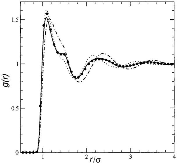
Molecular fluid: site-site correlation function g(r) for chlorine-like molecules (ℓ*=0.547) at reduced density ρ*=0.524, reduced screened density η*=ρ*/1.974, and reduced temperature T*=2.20. Dotted, dashed-dotted, and solid lines correspond to the the prediction of Dyer et al. (Ref. ⁴⁵), PISM-HNC prediction (Ref. ⁴⁰), and this work, respectively. Circles correspond to data simulation.

FIG. 4.

Molecular fluid: site-site correlation function g(r) for larger molecules (ℓ*=0.729) at reduced density ρ*=0.524, reduced screened density η*=ρ*/1.559, and reduced temperature T*=2.20. Solid line and circles correspond to this work and data simulation, respectively.

Let us first consider the optimization surface. We have performed a three dimensional optimization for each of the homonuclear diatomic examples using a simplex. In Fig. 5 we show a typical one-dimensional cut through the optimization surface by fixing two parameters at their optimum, namely, a^r=12.00 and a^b=8.6, and then plotting the chemical potential as a function of the remaining parameter a^o. We find the minimum around a^o=15.5. Convergence for correlation functions at values of a^o larger than 16 was not obtained due their highly oscillatory behavior. Indeed, the isothermal compressibility obtained for values of a^o much larger than the minimum becomes negative due to the behavior of the correlation function at long distances. These kinds of solutions also introduce errors in evaluating the Fourier transform of the direct correlation function at the origin, which is present in our analytical expression.

FIG. 5.

Optimization surface for the chemical potential as a function of the parameter a^o fixing a^r=12.00 and a^b=8.6 for the molecular system (ℓ*=0.547) at reduced density ρ*=0.524 and reduced temperature T*=2.20. Dashed line is the numerical quadrature and the dot dashed corresponds to our analytic approximation.

For the case with reduced bond length ℓ*≡L/σ=0.547 we have compared our prediction (solid line) for the site-site correlation function g(r)=1+h^o(r)+h^r(r)+h^ℓ(r)+h^b(r) with the ones provided by other proper approximate theories, namely, PISM-HNC prediction (dashed-dotted line), prediction of Dyer et al.⁴⁵ (dotted line), and with MD simulation (circles) in Fig. 3. In the case of the longer bond length ℓ*=0.729, we have compared our prediction (solid line) with simulation (circles) in Fig. 4. In both cases we conclude that our results are in near quantitative agreement with simulation data over the entire range. In fact, our theory does well with the notoriously difficult phase of oscillation at intermediate distances, in agreement with MD simulations in both models. Also the pronounced shoulder present in the chlorine-like model produced by the intramolecular correlations is well represented. A small difference between the simulation and our predictions is observed in the height of the first peak, where there is an underestimation of about 4%, for the phase points shown.

In reference to the optimization scheme we should point out that there is not a solution for Eqs. (20) and (15) for all of values of the three a parameters as previously mentioned. We have observed that the dominant behavior of the correlation function is determined by the parameter a^o, shown in Fig. 5, which weights that subclass of diagrams coming from the unbonded Mayer integral contributions. The others, which are more affected by the internal structure of the molecules, adjust the details of the shape of g(r).

We note that some care must be used in calculating the chemical potential. In particular, in Fig. 5 we show both our analytic approximation as well as an exhaustive quadrature. In particular, our calculations for the correlation functions and the chemical potentials have been performed using a step size in real space of 0.0175 Å and a fixed grid of 4096 points. As stated before the shape of the curves is quite close, however, the absolute value is displaced by a nearly constant amount in the region displayed.

Convergence of our procedure can be conveniently reached by providing a “good” initial guess of the values for the three a parameters. In this sense, a simple candidate is one in which all of them have the same value. From such a guess most minimization routines were able to find the minimum easily. The direct application of this algorithm to those two models generate the following values, minimizing the excess chemical potential: a^o=15.463, a^r=11.980, and a^b=8.595 for the chlorine-like model and a^o=0.2798, a^r=0.0096, and a^b=0.001 for the other one. Observe that we find a^o>a^r>a^b in both cases.

In Table I we have tabulated the numerical result for the excess internal energy U^ex/Nε obtained from the following formula:

$$\frac{U^{\mathrm{ex}}}{N\epsilon }=\frac{\rho }{2\epsilon }\underset{\alpha ,\gamma =0}{\overset{1}{\Sigma }}\int d\mathbf{r}{u}_{\alpha \gamma }\left(r\right)g_{\alpha \gamma }\left(r\right).$$ (22)

TABLE I.

Comparison between MD simulation and theoretical predictions for the excess internal energy U^ex/N_ε at reduced density ρ*=0.524 and reduced temperature T*=2.20. The excess chemical potential βμ_ex, predicted by several approximate theories, is also included in this table.

	CSL-HNC		Result of Dyer et al.		This work
Reduced bond length	Uex/Nε	βμex	Uex/Nε	βμex	Uex/Nε	βμexa	MD Uex/Nε
ℓ*=0.329	b	b	−13.88	−5.85	−13.70	−6.48	−14.31
ℓ*=0.547	−13.37	−4.34	−12.72	0.53	−12.47	−1.58	−12.38
ℓ*=0.729	−11.93	6.17	−11.20	9.13	−11.41	5.67	−11.52

^aResults obtained from the numerical evaluation of the Morita and Hiroike expression.

^bSee Ref. 44.

Comparisons are made with MD simulation and the different PISM-like theories. In computing integral (22) we have used the following cutoff r_max=6σ. We found that our predictions are in reasonable agreement with the simulation values.

Finally, it is well known that for RISM and PISM theories very short bond lengths are problematic. In this spirit, we have also analyzed a model with a shorter reduced bond length ℓ*=0.329 and reduced screened density η*=ρ*/2.646 corresponding to a molecule like N₂. In this case, the optimized parameters were found to be a^o=0.400, a^r=0.380, and a^b=0.073. While the first peak and its subsumed shoulder are remarkably well reproduced, we observe a phase mismatch between our prediction and data simulation for the midrange solvation shells (see Fig. 6). This behavior is, however, inherent to all of the known approximate theories based on diagrammatically proper integral equations, which, by construction, recover the correct united-atom limit with difficulty.⁴³

FIG. 6.

Molecular fluid: site-site correlation function g(r) for shorter molecules (ℓ*=0.329) at reduced density ρ*=0.524, reduced screened density η*=ρ*/2.646, and reduced temperature T*=2.20. Solid line and circles correspond to this work and data simulation, respectively.

All models studied for other thermodynamic states are not shown. We observed a smooth but not insignificant dependence on both temperature and density in the values of the a parameters.

VI. CONCLUSIONS

We have introduced a thermodynamically consistent theory which has been successfully tested on both simple and homonuclear diatomic Lennard-Jones fluids. Specifically, a closure approximation for simple fluids is obtained by using the Percus' functional expansion to first order in the density for a functional which depends on density, activity, and a parameter determined by free energy optimization using an approximate analytical expression for the excess chemical potential. Our approximation is shown to be capable of approximating simulation results over a wide range of thermodynamic states. In particular, a smooth transition interpolating PY and HNC closures is found to be useful. The molecular version is derived from an extension of that developed for simple fluids. The closure was coupled with a diagrammatically proper integral equation recently introduced.⁴⁵

The simplicity of the expressions involved in the resulting theory has allowed us to also obtain an approximate analytic expression for the molecular excess chemical potential which can be minimized to estimate the numerical value of the free parameters that defines the closure. The excellent agreement with simulation data reached for the site-site distribution function g(r) on representative models of a homonuclear diatomic Lennard-Jones makes this proposal a starting point for developing accurate approximate theories for more complex systems.

We showed that this optimized theory is capable of correctly describing not only the peaks and phase of oscillation with MD simulations but also the pronounced shoulder present in the chlorine-like model produced by the appreciable interference between intra- and intermolecular correlations. This is a contrast with other known methods. Apparently the success of this approach is largely due to the fact that, like a density functional approach, the best closure approximation to describe a specific molecular fluid is chosen variationally. In addition, we have seen that the optimal parametrization is not universal. It depends on the thermodynamic state and on the internal structure of the molecules.

Further work involves the extension of this theory to describe polar multicomponent fluids. Finally, it is worth mentioning that other closure approximations can be analogously developed for studying molecular fluids over other range of thermodynamic states, for instance, in the proximity of critical points, by introducing suitable approximations like the one done here for simple fluids.

References

- 1.Hansen JP, McDonald IR. Theory of Simple Liquids. 2nd ed. Academic; London: 1986. [Google Scholar]
- 2.Lee LL. Molecular Thermodynamics of Nonideal Fluids. Butterworths; Boston: 1988. [Google Scholar]
- 3.Gray CG, Gubbins KE. Theory of Molecular Fluids. Vol. 1. Oxford University Press; London: 1984. [Google Scholar]
- 4.Attard P. Thermodynamics and Statistical Mechanics: Equilibrium by Entropy Maximization. Academic; London: 2002. [Google Scholar]
- 5.Chandler D. In: The Liquid State of Matter: Fluids, Simple and Complex. Montroll EW, Lebowitz JL, editors. North-Holland; Amsterdam: 1982. p. 275. [Google Scholar]
- 6.Fantoni R, Pastore G. J. Chem. Phys. 2003;119:3810. [Google Scholar]
- 7.Percus JK, Yevick GJ. Phys. Rev. 1958;110:1. [Google Scholar]
- 8.Stell G. Physica (Amsterdam) 1963;29:517. [Google Scholar]
- 9.Morita T. Prog. Theor. Phys. 1960;23:829. [Google Scholar]
- 10.Verlet L. Nuovo Cimento. 1960;18:77. [Google Scholar]
- 11.Hoye JS, Stell G. J. Chem. Phys. 1977;67:439. [Google Scholar]
- 12.Lebowitz JL, Percus JK. Phys. Rev. 1961;122:1675. [Google Scholar]
- 13.Stell G. Mol. Phys. 1969;16:209. [Google Scholar]
- 14.Van Leeuwen JMJ, Groeneveld J, Deboer J. Physica (Amsterdam) 1959;25:792. [Google Scholar]
- 15.Zerah G, Hansen J. J. Chem. Phys. 1985;84:2336. [Google Scholar]
- 16.Sarkisov G. J. Chem. Phys. 2001;114:9496. [Google Scholar]
- 17.Rosenfeld Y, Ashcroft NW. Phys. Rev. A. 1979;20:1208. [Google Scholar]
- 18.Verlet L, Weis J. Phys. Rev. A. 1972;5:939. [Google Scholar]
- 19.Choudhury N, Ghosh SK. J. Chem. Phys. 2002;116:8517. [Google Scholar]
- 20.Bomont JM, Bretonnet JL. J. Chem. Phys. 2001;114:4141. [Google Scholar]
- 21.Duh D, Haymet ADJ. J. Chem. Phys. 1995;103:2625. [Google Scholar]
- 22.Foiles SM, Ashcroft NW. J. Chem. Phys. 1984;80:4441. [Google Scholar]
- 23.Martynov GA, Sarkisov GN. Mol. Phys. 1983;49:1495. [Google Scholar]
- 24.Rogers FJ, Young DA. Phys. Rev. A. 1984;30:999. [Google Scholar]
- 25.Ballone P, Pastore G, Galli G, Gazzillo D. Mol. Phys. 1986;59:275. [Google Scholar]
- 26.Verlet L. Mol. Phys. 1980;41:183. [Google Scholar]
- 27.Lee LL. J. Chem. Phys. 1995;103:9388. [Google Scholar]
- 28.Madden WG, Rice SA. J. Chem. Phys. 1980;72:4208. [Google Scholar]
- 29.Perkyns JS, Dyer KM, Pettitt BM. J. Chem. Phys. 2002;116:9404. [Google Scholar]
- 30.Dyer KM, Perkyns JS, Pettitt BM. J. Chem. Phys. 2002;116:9413. [Google Scholar]
- 31.Chandler D, Andersen HC. J. Chem. Phys. 1972;57:1930. [Google Scholar]
- 32.Ladanyi BM, Chandler D. J. Chem. Phys. 1975;62:4308. [Google Scholar]
- 33.Chandler D, Pratt L. J. Chem. Phys. 1976;65:2925. [Google Scholar]
- 34.Chandler D. Mol. Phys. 1976;31:1213. [Google Scholar]
- 35.Chandler D. J. Chem. Phys. 1977;67:1113. [Google Scholar]
- 36.Hirata F, Rossky PJ, Pettitt BM. J. Chem. Phys. 1983;78:4133. [Google Scholar]
- 37.Pettitt BM, Rossky PJ. J. Chem. Phys. 1983;78:7296. and references therein. [Google Scholar]
- 38.Jhonson E, Hazoume RP. J. Chem. Phys. 1979;70:1599. [Google Scholar]; Monson P. Mol. Phys. 1982;47:435. [Google Scholar]; Sullivan DE, Gray CG. Mol. Phys. 1981;42:443. [Google Scholar]; Cummings PT, Stell G. Mol. Phys. 1981;44:529. [Google Scholar]
- 39.Chandler D, Silbey R, Ladanyi B. Mol. Phys. 1982;46:1335. [Google Scholar]; Chandler D, Joslin CG, Deutch JM. Mol. Phys. 1982;47:871. [Google Scholar]
- 40.Rossky PJ, Chiles RA. Mol. Phys. 1984;51:661. [Google Scholar]
- 41.Lupkowski M, Monson PA. J. Chem. Phys. 1987;87:3618. [Google Scholar]
- 42.Lue L, Blankschtein D. J. Chem. Phys. 1995;102:5427. [Google Scholar]
- 43.Lue L, Blankschtein D. J. Chem. Phys. 1995;102:4203. [Google Scholar]
- 44.Dyer KM, Perkyns JS, Pettitt BM. J. Chem. Phys. 2005;122:236101. doi: 10.1063/1.1893829. [DOI] [PubMed] [Google Scholar]
- 45.Dyer KM, Perkyns JS, Pettitt BM. J. Chem. Phys. 2005;123:204512. doi: 10.1063/1.2116987. [DOI] [PMC free article] [PubMed] [Google Scholar]
- 46.Kirkwood JG. J. Chem. Phys. 1935;3:300. [Google Scholar]; Chem. Rev. (Washington, D.C.) 1936;19:275. [Google Scholar]
- 47.Morita T, Hiroike K. Prog. Theor. Phys. 1960;23:1003. [Google Scholar]
- 48.Lee LL. J. Chem. Phys. 1992;97:8606. [Google Scholar]
- 49.Kjellander R, Sarman S. J. Chem. Phys. 1989;90:2768. [Google Scholar]
- 50.Kast SM. Phys. Rev. E. 2003;67:041203. doi: 10.1103/PhysRevE.67.041203. [DOI] [PubMed] [Google Scholar]
- 51.Ryzhik G, Jeffrey A. Table of Integrals, Series, and Products. 5th ed. Academic; London: 1986. [Google Scholar]; Abramowitz M, Stegun IA. Handbook of Mathematical Functions. Dover; New York: 1972. [Google Scholar]
- 52.Hansen JP, Zerah G. Phys. Lett. 1985;108A:277. [Google Scholar]
- 53.Ornstein LS, Zernike F. Proc. Natl. Acad. Sci. U.S.A. 1914;17:793. [Google Scholar]
- 54.Lue L, Blankschtein D. J. Chem. Phys. 1994;100:3002. [Google Scholar]