Classification of parenchymal abnormality in scleroderma lung using a novel approach to denoise images collected via a multicenter study

INTRODUCTION

There are no widely accepted classification techniques to score the extent of interstitial lung disease in multicenter trials [1]. It is especially important to offer an accurate and robust pattern classifier to help produce quantitative disease measures for both clinical care and research applications [1, 2]. Although computer-generated texture features have been used to categorize interstitial lung disease patterns [3–7], many challenges in their standardization prevent widespread use. Different radiation-dose protocols and disparate reconstruction kernels hamper the standardization process [6].

Image noise is another factor that limits standardization, causing large variation in image quality. Image noise is affected by patient’s morphology, acquisition parameters, and computed tomography (CT) platforms. Removing noise (denosing) has been shown to be clinically relevant to detect subtle abnormalities, such as groundglass opacity of the lung, and to decrease interreader variability [8]. Radiation dose may be increased to improve CT signaling, which reduces noise, but safety concerns restrict this procedure. Noise may only be removed by postprocessing algorithms once the CT image is obtained.

Currently, two main methods exist for denoising images. The first is based on the wavelet coefficient of the image [9, 10], and the second is based on modeling patterns of noise and processing an iterative algorithm [11–13]. The approach of modeling pattern of noise has broad appeal since a distribution of model can be selected by pattern of noise, and the amount of noise can be set as noise parameter [13]. While Gaussian distributions characterize white noise [13–15], CT noise is not Gaussian. Under such circumstances, denoising CT images may be accomplished by modeling noise of oscillatory patterns in the negative Sobolev norm space or G space, which obviates normality [14]. Aujol’s iterative algorithm under G space is adaptable to non-Gaussian distribution of noise. This algorithm was used to decompose a digital image by separating noise under the estimated noise parameter, thus, creating two components: a denoised and a noise image component [15].

The purpose of this study is to investigate the utility of texture features from denoised versus original thin section CT image data in the classification of multiple patterns of scleroderma lung disease. Scleroderma patterns included lung fibrosis (LF), groundglass (GG), honeycomb (HC), as well as normal lung tissue (NL) from small region of interests. A potential advantage of denoising CT image data sets prior to classification is to allow data analysis from multiple platforms in multi-center trials.

MATERIALS AND METHODS

Image Denoising

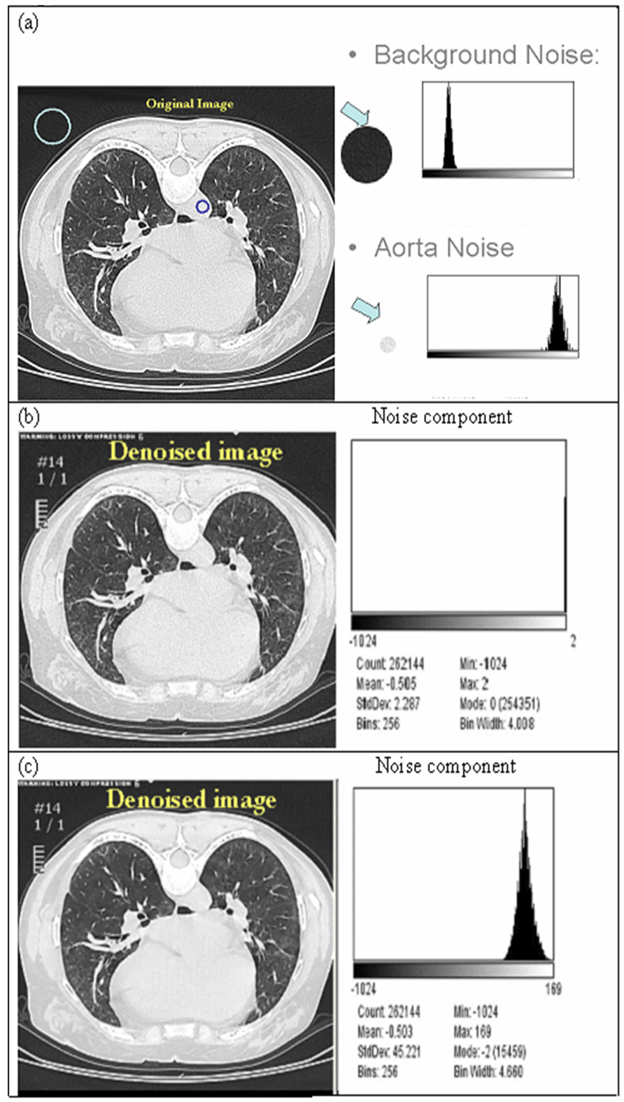
Before judging the utility of texture features in classification, we investigated the two main methods for denoising CT images. A noise parameter in the algorithm was estimated as standard deviation (std dev) of a region with expected uniform attenuation (in this study we used a region of interest placed in mid lumen of aorta) in CT image and all oscillatory patterns were considered to be indicative of noise (Fig 1.a.). As shown in Figure 1, the histogram of the original noise components from the mid lumen of aorta and background (Fig. 1.a) were not reproduced using the wavelet method (Fig 1.b.), which assumes a white noise distribution. When the CT image was denoised with Aujol’s method [15], the histogram from the aorta region (Fig. 1.c), which estimates the noise component, was similar in shape to its original. Details of Aujol’s algorithm are listed in appendix 1 and 2.

Figure 1.

Noise characteristics in a CT image. (a) Original CT image and histogram from background and aorta. (b) Denoised image and frequency histogram of the noise image from decomposed algorithm [15] assuming that the noise in CT is white noise. (c) Denoised image and frequency histogram of the noise image from the decomposed algorithm [15, 17] assuming that the noise in CT is non-white noise.

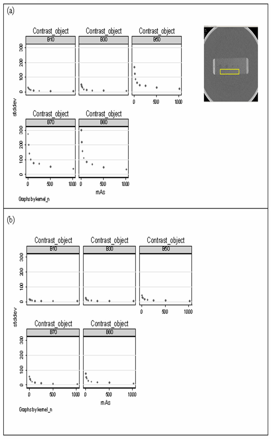
We then examined the robustness of Aujol’s method to denoise CT images with varying dose levels and reconstruction kernels. We denoised contrast phantom images that were scanned at dose levels ranging from 8–1024 mAs and acquired under different reconstruction kernels ranging from smooth to over-enhancing. We measured the std dev of pixels over a homogenous region and demonstrated that std dev from denoised images were smaller and more consistent than those obtained from original images regardless of dose or kernel (Fig. 2).

Figure 2.

Scatter plot of texture feature, standard deviation (std dev) on various dose level by different kernel from (a) original image and (b) denoised image. The dose level ranged from 8 mAs to 1024 mAs. The kernel of B10, B30, B50, B70, and B80 stand for smooth, standard, sharp, very sharp, and over-enhanced kernel, respectively.

Scleroderma Lung Study

The Scleroderma Lung Study (SLS) was a multicenter NIH-sponsored randomized controlled trial comparing cyclophosphamide with placebo. The study started in 2000 and involved 13 clinical centers throughout the United States (U01 HL60587-01A1, for detail, see Tashkin et al [16]). Briefly, patients had baseline thoracic high-resolution computed tomography (HRCT) scans in prone position at total lung capacity (TLC). The images were acquired on 13 scanner models from 4 manufacturers (ELSCINT, General Electric, Picker International Inc, and Siemens). The actual exposure in the study ranged from 80 mAs to 380 mAs (mean of 245mAs with std dev 79). The peak tube current potentials were 120 kVp, 130 kVp, and 140 kVp. Scans were acquired incrementally with 10mm gaps of 1–2 mm slice thickness and were not volumetric. In general, the CT scans were reconstructed with high spatial frequency reconstruction kernels (bone for General Electric and B45 or B70 for Siemens).

Sub Study Data

From baseline scan, a training set of 38 consecutive patients was chosen, and from within theses patients, 148 regions of interest (ROIs) that demonstrate classic, homogeneous and unambiguous features of SLS disease patterns and normal lung tissue were contoured. (See Contouring below). Regions included 46 LF, 85 GG, 4 HC, and 13 NL patterns. Next, 132 ROIs from a test set of 33 independent patients were contoured using identical criteria in order to evaluate the classification ability of the model built on the training set. Test regions included 44 LF, 72 GG, 4 HC, and 12 NL patterns.

The number of ROIs selected from a single patient ranged from 1 to 11. Within each ROI, grids composed of 4-by-4 pixel squares were placed contiguously. From each grid, a pixel was selected by algorithm (4-by-4 grid sampling). Grid sampling was used to assure complete ROI coverage for each disease pattern type. Due to the nature of the grid sampling scheme, the number of sampled pixels was directly proportional to the ROI’s size. For example, if the number of pixels in a squared ROI is 16, the scheme chooses 1 pixel, whereas 10 pixels are selected from a rectangular 160-pixel ROI. In total, 5690 (3009 LF, 1994 GG, 348 HC, 339 NL) pixels and 5045 (2665 LF, 1753 GG, 291 HC, 336 NL) pixels were sampled in the training and test sets, respectively. The disease class of each sampled pixel was assumed to equal the overall ROI disease type as labeled visually. Table 1 summarizes the study data.

Table 1.

Summary of training and test datasets (ROI: Region of interests, LF: Lung Fibrosis, GG: Groundglass, HC: Honeycomb, NL: Normal Lung).

Numbers	Patients	Contoured ROIs	Grid sample pixels
Training set	38	148 (46 LF, 85 GG, 4 HC, 13 NL)	5690 (3009 LF, 1994 GG, 348 HC, 339 NL)
Test set	33	132 (44 LF, 72 GG, 4 HC, 12 NL)	5045 (2665 LF, 1753 GG, 291 HC, 336 NL)

Contouring

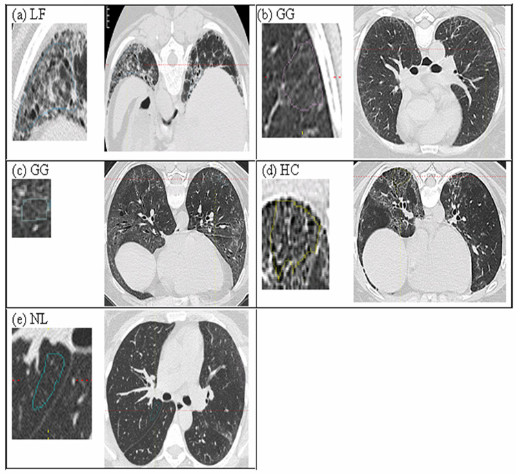
A single thoracic radiologist [JGG] with 12 years of experience visually contoured all ROIs in both training and test sets (This radiologist, a member of a consensus-reading panel, provided standardized examples of LF, GG, HC, and NL regions for the initial study by Tashkin et al [16].). The visual characteristics of the four classes of images (3 abnormalities plus NL) are illustrated in Figure 3. For completeness, pure GG (Panel b) and GG with adjacent LF (Panel c) were combined into a single class when investigating texture-feature utility in original versus denoised images.

Figure 3.

Disease pattern and normal lung tissue in thin-section CT scans of the chest. An enlarged view of contoured ROI is shown on the left side of each image. (a) Lung Fibrosis (LF): Destruction of the lung parenchyma of reticular opacification, traction bronchiectasis and bronchiolectasis with increasing attenuation [16]. (b) Pure Groundglass (i.e. Groundglass without distortion): Destruction of the lung parenchyma moderately increased attenuation homogeneously in the absence of LF [16]. (c) Groundglass with adjacent LF: Groundglass that is located adjacent to LF. (d) Honeycomb (HC): clustered air-filled cysts with dense walls [16] (e) Normal lung tissue (NL): The mean CT attenuation value of the lung parenchyma is lower than that of disease cases.

Classification Procedures and Statistical Analyses

To compare classification performances using texture features from original and denoised CT images, the following steps were performed:

1. Denoise the CT image that contains the contoured ROI. Aujol’s denoise algorithm [15] was implemented by setting the noise parameter, as the std dev of aorta. Details of the algorithm are given in Appendix 1 and 2

2. Sample each pixel from the 4-by-4 grid within the ROI.

3. Calculate the texture features from original and denoised CT image for the sampled pixel. Fifty-eight texture features including statistical features, run-length parameters, and co-occurrence parameters were calculated [18, 19].

4. Repeat (1) to (3) for all sampled pixels from 148 contoured ROIs drawn from 38 patients in the training set. Yielded texture measurements on 5690 (3009 LF, 1994 GG, 348 HC, 339 NL) pixels.

5. Select important texture features from the training set using multinomial logistic model. We selected the important features using multinomial logistic regression with backward selection where the cut-off value was set to p=0.10 for multi-class categories [20]. A feature was selected if it was significantly associated for at least one of the classification categories. Regressions were implemented using Stata V.9.0 (College Station, Texas 77845 USA).

6. Model support vector machine (SVM) classification using the selected texture features from the training set. Features from Step 5 were used as predictors to build classification models via SVM. (SVM was initially developed by Vapnik [21] and has been shown to perform well in medical imaging studies [22, 23], especially pattern recognition of interstitial lung disease [6].) The basic idea involves finding support vectors that maximize the margin between classes. To maximize the margin, a kernel (shape of separating hyperplane) and a cost of misclassification need specification. In our experience, a radial basis kernel with cost 1 optimized the classification rates for both original and denoised image data. SVM classification was implemented using R Version 2.2.1.

7. Repeat (1) to (3) for sampled pixels from 132 contoured ROIs drawn from 33 patients in the test set. Yielded texture features measurements on 5045 (2665 LF, 1753 GG, 291 HC, 336 NL) pixels.

8. Fit the previous built SVM classifier to the test set using the same selected texture features. The test set of texture features from contoured ROIs was then used to assess the prediction accuracy of SVM from Step (6).

9. Report tables of classification results on pixels as well as ROIs and compare the classification rates. Based on support vectors from selected features in the training set, the pixels from training and testing sets were classified as multi-categorical disease types. For the purpose of pixel classification rates, the “truth” of all pixels within a contoured ROI was assumed to be equal to its visual label. (Pixel-level p-values for classification rates were not provided since their calculation was problematic, requiring the estimation of numerous and complex covariance structures–one for each ROI). The ROI classification rate was estimated as the ratio of the total number of correctly classified pixels from the ROI to the total number of sampled pixels from the ROI. For each ROI, its overall classification type by SVM was chosen by majority vote from corresponding sampled pixel classifications. Differences in ROI classification rates from original and denoised CT image data were compared by the paired t-tests. (By the nature of our study design, tests for significance at ROI level should lead to more robust findings since they are not as susceptible to possible dependency assumptions). To mitigate problems arising from small numbers of NL ROIs, NL classification rates were compared via a bootstrap test. Differences in the distributions of false-positive counts per ROI between original and denoised images in the test set were assessed using a random-effects Poisson regression test.

RESULTS

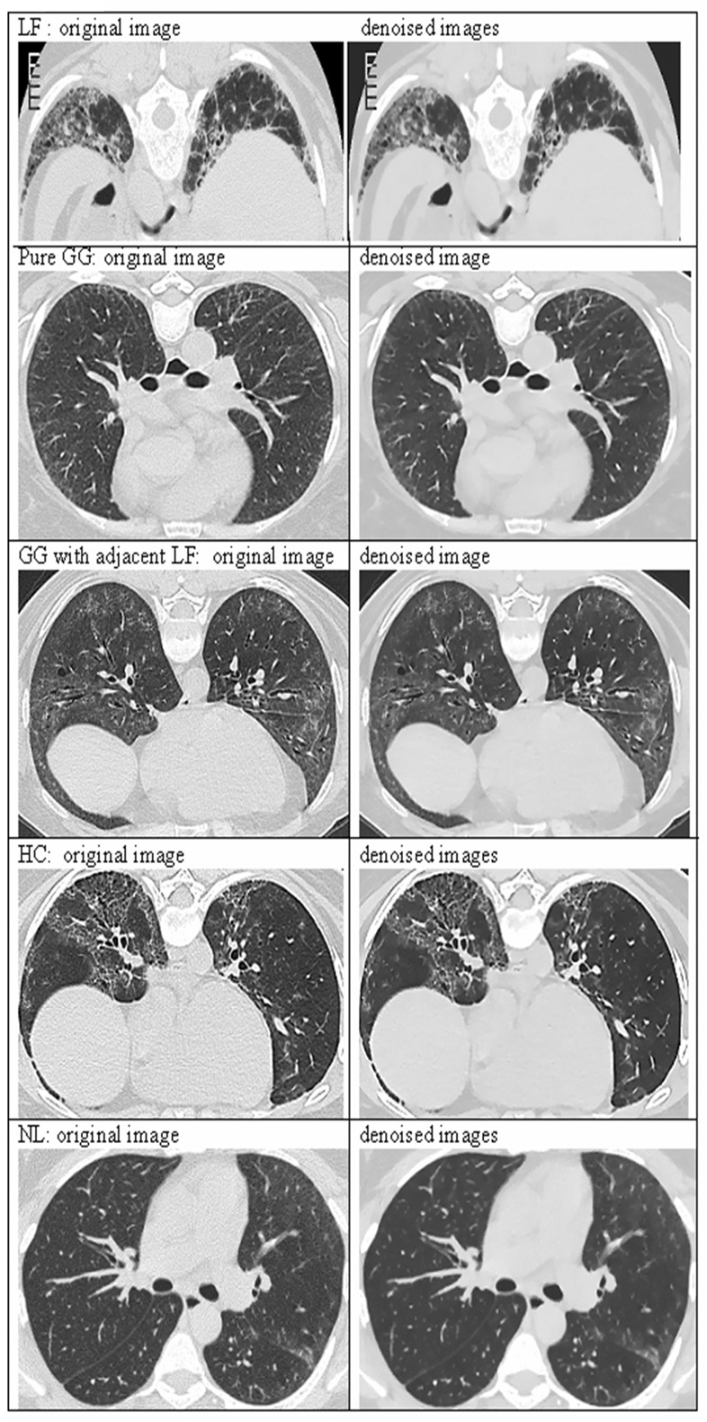
Representative results of implementing Aujol’s algorithm to denoise CT image data are shown in Figure 4. The image pairs correspond to the original and denoised examples of abnormalities (LF, GG and HC) and normal tissue (NL) shown in Figure 3. In original images, the noise parameter equaled 50, which was the upper bound of std dev in the aorta across all patients.

Figure 4.

Comparison between original and denoised images from Figure 3.

From the training set, our logistic model selected 45 and 38 texture features from original and denoised images, respectively, as significant predictors of disease type. After finding disease-type boundaries based on vectors of the selected features (SVM), the observed pixel classification rates in the training set were 95.0% and 94.9% in original and denoised images, respectively. Individually, the specificity of LF was lowest (original image = 2517/2681 or 93.9%; denoised image = 2522/2681 or 94.1%), and HC demonstrated the highest specificity (original image = 5324/5342 or 99.7%; denoised image = 5321/5342 or 99.6%). At the ROI level, the mean classification rates from original and denoised images were not significantly different (p=0.71, data not shown).

Table 2 and Table 3 present the pixel-level classification results from original and denoised images in the test set, respectively. From the values, disease-type specificities (in the original and denoised images) can be derived. In general, denoised specificities were larger than their original counterparts. For example, the specificities ranged from 83.5% (1556/2380) for LF to 99.7% (4696/4709) for NL.

Table 2.

Test set of classification result on ROI using original features with SVM model for four patterns: LF, GG, HC, and NL.

	Original Texture Feature
	LF	GG	HC	NL	Total
True class
LF	2567	76	22	0	2665
GG	184	1556	0	13	1753
HC	208	21	62	0	291
NL	0	89	0	247	336

Table 3.

Test set of class classification result on pixel using denoised features with SVM model for four patterns: LF, GG, HC, and NL.

	Denoised Texture Feature
	LF	GG	HC	NL	Total
True class
LF	2569	72	24	0	2665
GG	164	1567	2	20	1753
HC	198	7	84	2	291
NL	0	39	0	297	336

The numbers of false-positive original pixels (off-diagonal counts in Table 2) were generally greater than corresponding denoised values (Table 3). For example, the number of false positive NL pixels changed from 89 in original images to 39 in denoised images. From distributions of false-positive counts per ROI, original false-positives exceeded denoised false-positives (p=0.004). In particular, 5 fewer NL false-positive counts per ROI were observed in average after denoising the images (p=0.001).

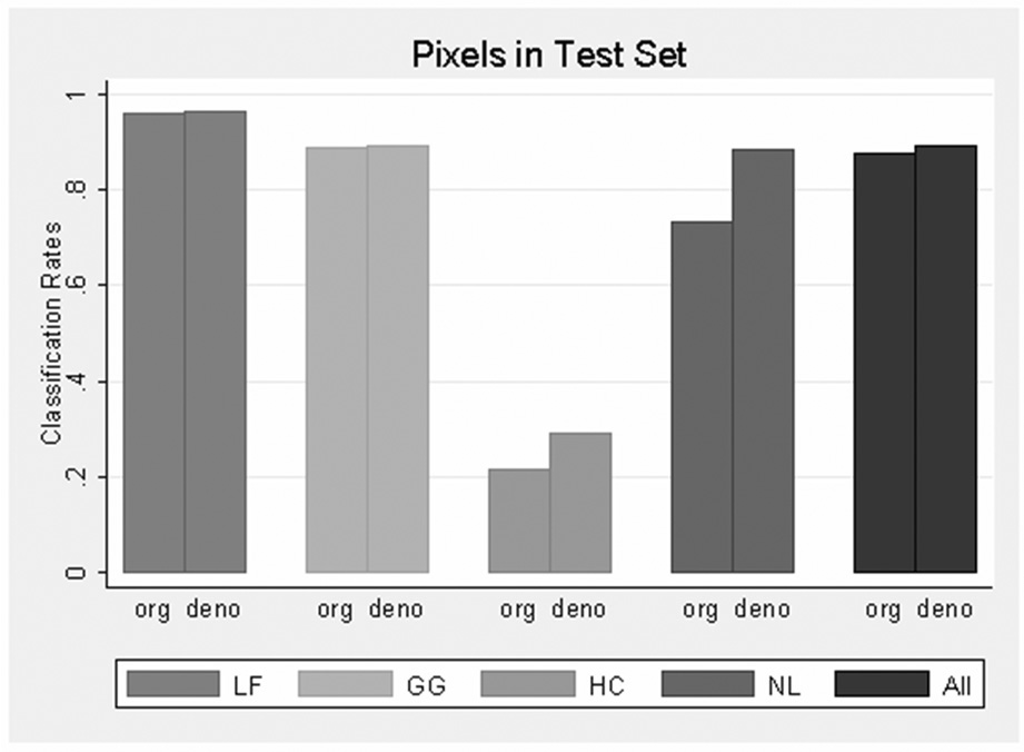
Figure 5 presents overall pixel-level classification rates, as well as disease type and NL pattern rates from original and denoised features in the test sets. Overall accuracies in the test set were 87.8% (4432/5045) and 89.5% (4517/5045) for original and denoised features, respectively. Most of the increase (denoised vs. original) was attributed to the higher rate of correct classification of NL pixels (88.4% in denoised images vs. 73.5% in original images).

Figure 5.

Pixel classification rate in test set of features from original and denoised images by disease pattern and all type. “org” and “deno” represent texture features from original and denoise image respectively.

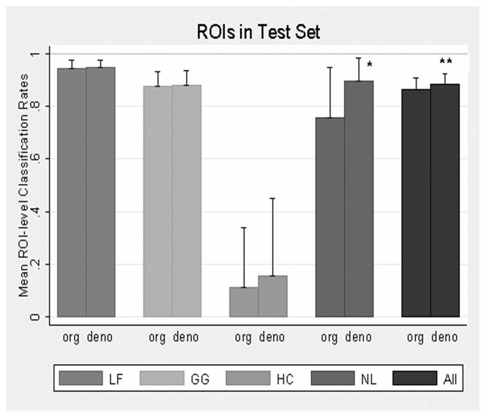
Figure 6 presents mean ROI-level classification rates and their upper bound confidence limits from the original and denoised features in the test sets. The difference between original (86.7%) and denoised (88.4%) average classification rates was significant (p=0.047), and again, most of the change was attributed to a significant (p = 0.037) increase in the average classification of NL tissue (75.9% for original images vs. 89.7% for denoised images). Regarding LF and GG ROIs, high (near 90%) mean classification rates were not changed by denoising, and for HC, a poor (<20%) classification was not improved by denoising.

Figure 6.

Mean ROI classification rate from test set of features from original and denoised images by disease pattern and all type. “org” and “deno” represent texture features from original and denoise image respectively. Error bars represent standard error of upper bound confidence limits. There was significant differences in NL (*: p=0.037) and overall (**: p=0.047)

Table 4 and Table 5 present test-set counts of ROI types cross-classified according to their visual and SVM majority-vote labels (Table 4 shows contingencies based on original features, and Table 5 shows denoised values). More misclassification errors arose using original features (1 LF, 6 GG, 4 HC and 2 NL errors) compared with denoised features (0 LF, 5 GG, 4 HC and 0 NL errors). LF and NL types were 100% correctly classified using the denoised features.

Table 4.

Test set of classification result on ROI by majority vote for four patterns: LF, GG, HC, and NL.

	Original Texture Feature
	LF	GG	HC	NL	Total
True class by the radiologist
LF	43	1	0	0	44
GG	6	66	0	0	72
HC	4	0	0	0	4
NL	0	2	0	10	12

Table 5.

Test set of classification result on ROI by majority vote for four patterns: LF, GG, HC, and NL.

	Denoised Texture Feature
	LF	GG	HC	NL	Total
True class by the radiologist
LF	44	0	0	0	44
GG	5	67	0	0	72
HC	4	0	0	0	4
NL	0	0	0	12	12

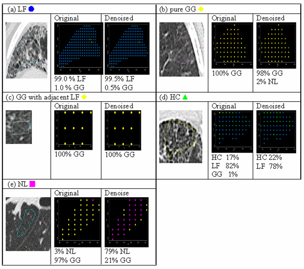
Figure 7 illustrates the potential of our procedure to better quantify heterogeneous disease patterns within lungs. Although ROIs (Panels a–e) were visually labeled as homogeneous, our classifier almost always assigned disease mixtures, which were altered by denoising. In particular, Panels b and e highlight these alterations where yellow and pink pixels represent the classifications GG and NL, respectively. In Panel b, all pixels in the original image were classified as GG, which agreed with the visual label. However, once denoised, 2% of pixels were also classified as NL. In contrast, only 3% of pixels in Panel e were classified as NL (the visual label) using original features, but 79% of pixels were classified as NL using denoised features.

Figure 7.

Comparison of Pixel SVM Classifications by original and denoised features using the ROIs from Figure 3. Legend: LF , GG , HC , NL .

Note that image sizes were rescaled subjectively. Each dot represented the same size of pixel, which was sampled by rule of one out of 4-by-4 neighboring pixels.

DISCUSSION

Computational approaches have been used to classify disease patterns in the lung, but none have investigated the influence of noise on classification accuracy. To date, most classification models are based on image data sets derived from a single platform and thus, may not be generalizable to images acquired on different platforms or to using different imaging protocols even on the same platform [3–7]. CT image noise can be influenced by the technique used: the product of tube current and time (mAs), slice thickness, beam energy (KVp), and patient specific factors (size, breathing, etc) [25]. Because the object is scanned with noise, these different factors can result in the same object of interest or ROI having different texture features, which in turn leads to unstable classifiers. Texture features from a denoised image can be useful in multicenter trials for classification of interstitial lung diseases since it further standardizes uncontrollable noise as postprocessing before classifying the patterns of diseases.

Many different classification methods have been applied to distinguish patterns of disease in the lungs using texture features [3–7]. The Adaptive Multiple Feature Method (AMFM) assessed patterns of HC, GG, bronchovascular, nodular, emphysema-like, and NL tissues using as many as 22 independent texture features [3]. A supervised Bayesian classifier differentiated obstructive lung diseases as centrilobular emphysema, panlobular emphysema, constrictive obliterative bronchiolitis and NL using 13 texture features [4]. Artificial neural networks assessed localized GG opacity using five texture features and Gaussian curve fitting features [5]. SVM has been applied to classify emphysema, GG, HC, and NL tissues using fractal and 3D texture features, which were implemented in AMFM [6]. Finally, adaptive histogram binning and the canonical signatures were applied to the classification of HC, reticular, GG, NL, and emphysema [7]. In this study, Zavaletta et al also demonstrate that reticular and HC may be considered together to quantify LF in patients with moderate usual interstitial pneumonitis or idiopathic pulmonary fibrosis [7].

Here, we considered jointly a multinomial logistic model for variable selection and the use of SVM to classify LF, GG, HC and NL patterns in patients with scleroderma lung disease. Multinomial logistic regression allowed for multiple category classifications [18], and SVM has excellent efficacy for high-dimensional data while requiring minimal assumptions in the texture feature space [19]. Moreover, the SVM algorithm is typically superior to standard discriminant analysis and other neural networks [20]. For completeness, we also investigated classification using predicted probabilities from a multinomial model itself; however, we do not report or discuss the results since this procedure led to similar conclusions as SVM with lower classification rates.

This study was unique since texture features were derived from both original and denoised images. We found that classification based on the denoised images had two main advantages:

1. Parsimony – numbers of features selected from training sets were reduced by 7 from 45 to 38 comparing original and denoised images, respectively.

2. Accuracy – overall and NL classification rates were higher when using denoised test set data.

Principally, denoising reduced measurement error permitting fewer features to classify disease types, and fewer features reduced bias associated with classification. NL classification improved the most (Figure 6), and this observation meets expectations.

Aujol’s denoising algorithm reduces large oscillatory patterns, and thus, attenuation of adjoining pixels will appear more uniform, causing true normal tissue to appear more “black”. Furthermore, NL patterns in scleroderma patients are typically located more central than peripheral, where noise is more likely to be encountered (i.e., larger oscillatory patterns as a function of X-ray distance). In Figure 7, Panel e is an exemplary patient showing NL improvement with denoising when the ROI was located in the center of the lung. In contradistinction, classification of diffuse scleroderma characteristics, such as LF and GG, should be less impacted by any method, which generates uniformity.

We also expected denoising to substantially improve the classification of HC since sharpening areas would help focus patterns of uniform “black” delineated by “white” hexagonal boundaries. Yet, HC classification rates were poor (Figure 5 and Figure 6). Previous studies have shunned the classification of HC by regrouping HC as a form of LF [7]. Unfortunately, our study design lacked sufficient power to fully investigate this phenomenon. Power was dampened by high intraclass correlations among HC pixels, coming from relatively few subjects and ROIs [26, 27]. In addition, grid sampling likely underrepresented hexagonal HC boundaries, which vary and enlarge over time [28]. Without appropriate pixels in the feature space, the selection of textures that differentiated HC is wanted.

Our study had other limitations. First, the number of contoured ROIs was small, leading to unbalanced numbers of disease types. As a result, many more pixels were available to train and classify GG and LF relative to NL and HC. Second, the ROI size and shape hindered the reliable estimation of pixel-level covariance structures so that pixel-level classification rates could not be assessed (Statistical significance tests were performed only for the independent ROIs and for counts of false positive pixels across ROIs according to their visual labels). Third, our disease ROIs lacked pathological support, and in practice, some scleroderma disease patterns are difficult to differentiate, especially the truth between GG and NL. Hence, our radiologist was required to select only classic, homogeneous and unambiguous examples of disease patterns in order to detect definite normality and definite abnormality [29, 30], which possibly produced a selection bias and limited our findings. Fourth, we measured features in 2D only since our slice intervals (10mm) were not conducive to 3D estimation. 3D texture features have been shown to improve classification rates in lung disease [6].

In the future, we plan to investigate the use of denoised 3D texture features and structural attributes for better scleroderma disease classification. Additionally, our model can be adapted to utilize computer-aided systems (which reduce intra scanner variation) and applied to equalize reader performance [31]. Finally, the method can be extended to other types of interstitial lung disease.

CONCLUSION

Accurate and robust computerized classifications based on texture features appear improved when using denoised images. This is particularly important to discriminate normal from abnormal parenchyma given that GG and other disease patterns can be mimicked by image noise, leading to false positives. Based on this initial work that has a limited number of disease types, our CT denoising method yielded higher rates of correct normal lung tissue classification in scleroderma patients. Texture features from a denoised image with an SVM classifier have the potential to accurately discriminate different lung disease patterns and will be the subject of future research.

Appendix 1

Modified Aujol’s Algorithm [15]

1. Initialization:

   $$u_0=0$$
2. Iterations:

   $$w_{\mathrm{n}+1}=P_{\delta B_G}(f-u_n)$$

   $$u_{\mathrm{n}+1}=\mathrm{f}-w_{\mathrm{n}+1}-P_{\mathrm{\lambda }{B}_G}(f-w_{n+1})$$
3. Stopping test: we stop if

   $$\text{max}(|u_{\mathrm{n}+1}-u_{\mathrm{n}}|,|w_{\mathrm{n}+1}-w_{\mathrm{n}}|)\le \mathrm{\epsilon },$$

   where u and w represents the denoised and noised images, respectively, P_BG is a nonlinear projection described in appendix 2, and δ represents the amount of noise and λ represents the accuracy of algorithm. The sum of u and w is approximately equal to original CT image if the algorithm converges. Here, for the sake of simplicity, we set the noise parameter (δ) as 50, which was the upper bound of standard deviation in aorta across patients. Because the parameter has a certain threshold, the results of denoised images are similar to the values above the threshold. The residual parameter (λ) was set to 1, which controls the convergence of the algorithm.

Appendix 2

Any computerized image can be discretized into N by N vectors. And each element of a matrix is a pixel. We denote by X by Euclidian space R^NxN and de note Y=X×X. In CT image, the window size is 512 by 512.

Projection

Each element of P, projection matrix is below. And it was solved by a fixed point method [15, 17]:

$${\mathrm{p}}^0=0$$

and

$${\mathrm{p}}_{\mathrm{i},\mathrm{j}}^{\mathrm{n}+1}=\frac{{\mathrm{p}}_{\mathrm{i},\mathrm{j}}^{\mathrm{n}}+\mathrm{\tau }{(\nabla ({\text{div}(\mathrm{p}}^{\mathrm{n}})-\mathrm{f}/\mathrm{\lambda }))}_{\mathrm{i},\mathrm{j}}}{1+\mathrm{\tau }|\nabla ({\text{div}(\mathrm{p}}^{\mathrm{n}})-\mathrm{f}/\mathrm{\lambda }){)}_{\mathrm{i},\mathrm{j}}|}$$

Theoretically, this projection converge τ≤1/8. Practically, the author used ¼ and he stated that it worked better [15, 17].

Gradient Operator

Defining a discrete total variation, they introduced a discrete version of the gradient operator. If u ∈ X, the gradient ∇u is a vector in Y given by: ${(\nabla \mathrm{u})}_{\mathrm{i},\mathrm{j}}=({(\nabla \mathrm{u})}_{\mathrm{i},\mathrm{j}}^1,{(\nabla \mathrm{u})}_{\mathrm{i},\mathrm{j}}^2))$ [17].

Using

$${(\nabla \mathrm{u})}_{\mathrm{i},\mathrm{j}}^1=\{\begin{array}{cc}{\mathrm{u}}_{\mathrm{i}+1,\mathrm{j}}-{\mathrm{u}}_{\mathrm{i},\mathrm{j}}\hfill & \text{if}\mathrm{i}<\mathrm{N}\hfill \\ 0\hfill & \text{if}\mathrm{i}=\mathrm{N}\hfill \end{array}$$

and

$${(\nabla \mathrm{u})}_{\mathrm{i},\mathrm{j}}^2=\{\begin{array}{cc}{\mathrm{u}}_{\mathrm{i},\mathrm{j}+1}-{\mathrm{u}}_{\mathrm{i},\mathrm{j}}\hfill & \text{if}\mathrm{j}\text{<}\mathrm{N}\hfill \\ 0\hfill & \text{if}\mathrm{i}=\mathrm{N}\hfill \end{array}$$

,

Divergence Operator

They defined it by analogy with the continuous setting by div = − ∇*, where ∇* is the adjoint of ∇: that is, foe every p ∈ Y, and u ∈ X, (−div p, u)_x= (p, ∇u)_Y.

$${(\text{div}(\mathrm{p}))}_{\mathrm{i},\mathrm{j}}=\{\begin{array}{cc}\hfill {\mathrm{p}}_{\mathrm{i},\mathrm{j}}^1-{\mathrm{p}}_{\mathrm{i}-1,\mathrm{j}}^1\hfill & \hfill \text{if}1<\mathrm{i}<\mathrm{N}\hfill \\ \hfill {\mathrm{p}}_{\mathrm{i},\mathrm{j}}^1\hfill & \text{if}\mathrm{i}=1\\ \hfill -{\mathrm{p}}_{\mathrm{i}-1,\mathrm{j}}^1\hfill & \hfill \text{if}\mathrm{i}=\mathrm{N}\hfill \end{array}+\{\begin{array}{cc}\hfill {\mathrm{p}}_{\mathrm{i},\mathrm{j}}^2-{\mathrm{p}}_{\mathrm{i},\mathrm{j}-1}^2\hfill & \hfill \text{if}1<\mathrm{j}<\mathrm{N}\hfill \\ \hfill {\mathrm{p}}_{\mathrm{i},\mathrm{j}}^2\hfill & \hfill \text{if}\mathrm{j}=\mathrm{1}\hfill \\ \hfill -{\mathrm{p}}_{\mathrm{i},\mathrm{j}-1}^2\hfill & \hfill \text{if}\mathrm{j}=\mathrm{N}\hfill \end{array}$$

REFERENCES

- 1.Best AC, Lynch AM, Bozic CM, et al. Quantitative CT indexes in idiopathic pulmonary fibrosis: relationship with physiologic impairment. Radiology. 2003;228:407–414. doi: 10.1148/radiol.2282020274. [DOI] [PubMed] [Google Scholar]
- 2.Lynch DA. Quantitative CT of fibrotic interstitial lung disease. Chest. 2007;131:643–644. doi: 10.1378/chest.06-2955. [DOI] [PubMed] [Google Scholar]
- 3.Uppaluri R, Hoffman EA, Sonka M, et al. Computer recognition of regional lung disease patterns. Am J Respir Crit Care Med. 1999;160:648–654. doi: 10.1164/ajrccm.160.2.9804094. [DOI] [PubMed] [Google Scholar]
- 4.Chabat F, Yang GZ, Hansell DM. Obstructive lung diseases: texture classification for differentiation at CT. Radiology. 2003;228:871–877. doi: 10.1148/radiol.2283020505. [DOI] [PubMed] [Google Scholar]
- 5.Kim KG, Goo JM, Kim JH, et al. Computer-aided diagnosis of localized ground-glass opacity in the lung at CT: initial experience. Radiology. 2005;237:657–661. doi: 10.1148/radiol.2372041461. [DOI] [PubMed] [Google Scholar]
- 6.Xu Y, van Beek EJ, Hwanjo Y, et al. Computer-aided classification of interstitial lung diseases via MDCT: 3D adaptive multiple feature method (3D AMFM) Acad Radiol. 2006;13:969–978. doi: 10.1016/j.acra.2006.04.017. [DOI] [PubMed] [Google Scholar]
- 7.Zavaletta VA, Bartholmai BJ, Robb RA. High resolution multidetector CT-aided tissue analysis and quantification of lung fibrosis. Acad Radiol. 2007;14:772–787. doi: 10.1016/j.acra.2007.03.009. [DOI] [PMC free article] [PubMed] [Google Scholar]
- 8.Abtin F, Goldin JG, Suh R, Kim H, Ochs R, Brown MS, Gjertson D. Denoising of CT images for better detection and visualization of subtle parenchymal changes using novel Aujol and Chambolle algorithms and image decomposition. Oral presentation, scientific session, RSNA. 2006 [Google Scholar]
- 9.Donoho DL, Johnstone I. Adapting to unknown smoothness via wavelet shrinkage. J Am Stat Assoc. 1995;90:1200–1224. [Google Scholar]
- 10.Mallat SG. A wavelet tour of signal processing. San Diego, CA: Academic Press; 1998. [Google Scholar]
- 11.Rudin LI, Osher S, Fatemi E. Nonlinear total variation based noise removal algorithms. Physica D. 1992;60:259–268. [Google Scholar]
- 12.Nikolova M. A variational approach to remove outliers and impulse noise. J Math Imaging Vision. 2004;20:99–120. [Google Scholar]
- 13.Aujol JF, Gilboa G, Chan T, et al. Structure-texture image decomposition-modeling, algorithm, and parameter selection. Int J Comput Vision. (in press) [Google Scholar]
- 14.Yves Meyer. The fifteenth dean Jacquelines B. Lewis memorial lectures. Vol 22. Providence, RI: American Mathematical Society; 2001. Oscillating patterns in image processing and in some nonlinear evolution equations. [Google Scholar]
- 15.Aujol JF, Chambolle A. Dual norm and image decomposition models. Int J Comput Vision. 2005;63:85–104. [Google Scholar]
- 16.Tashkin DP, Elashoff R, Clements PJ, et al. Cyclophosphamide versus placebo in scleroderma lung disease. N Engl J Med. 2006;354:2655–2666. doi: 10.1056/NEJMoa055120. [DOI] [PubMed] [Google Scholar]
- 17.Chambolle A. An algorithm for total variation minimization and applications. J Math Imaging. 2004;20:89–97. [Google Scholar]
- 18.Sonka M, Hlavac V, Boyle R. Image processing, analysis and machine vision. London, England: Chapman & Hall; 1993. [Google Scholar]
- 19.Haralick RM, Shanmugam K. Texture features for image classification. IEEE Trans Syst Man Cybernetics. 1973;3:610–621. [Google Scholar]
- 20.Scott Long J. Regression models for categorical and limited dependent variables. Thousand Oaks, CA: Sage; 1997. [Google Scholar]
- 21.Vapnik VN. The nature of statistical learning theory. New York: Springer; 1999. [DOI] [PubMed] [Google Scholar]
- 22.Maglogiannis IG, Zafiropoulos EP. Characterization of digital medical images utilizing support vector machines. BMC Med Inform Decis Mak. 2004;4:4–32. doi: 10.1186/1472-6947-4-4. [DOI] [PMC free article] [PubMed] [Google Scholar]
- 23.Chapelle O, Haffner P, Vapnik V. Support vector machines for histogram based image classification. IEEE Trans Neural Networks. 1999;10:1055–1064. doi: 10.1109/72.788646. [DOI] [PubMed] [Google Scholar]
- 24.Efron B, Tibshirani RJ. Monographs on Statistics and Applied Probability. Boca Raton, FL: Chapman & Hall; 1993. An introduction to the bootstrap. [Google Scholar]
- 25.McNitt-Gray M. AAPM/RSNA physics tutorial for residents: topics in CT. Radiation dose in CT. Radiographics. 2002;22:1541–1553. doi: 10.1148/rg.226025128. [DOI] [PubMed] [Google Scholar]
- 26.Kish L. Survey Sampling. New York: John Wiley & Sons; 1965. [Google Scholar]
- 27.Snijders TAB, Bosker RJ. Standard errors and sample sizes for two-level research. J of Ed Statis. 1993;18:237–259. [Google Scholar]
- 28.Lynch DA, Travis WD, Müller NL, et al. Idiopathic interstitial pneumonias: CT features. Radiology. 2005;236:10–21. doi: 10.1148/radiol.2361031674. [DOI] [PubMed] [Google Scholar]
- 29.Remy-Jardin M, Remy J, Giraud F, Wattinne L, Gosselin B. Computed tomography assessment of ground-glass opacity: semiology and significance. Journal of thoracic imaging. 1993;8(4):249–264. doi: 10.1097/00005382-199323000-00001. [DOI] [PubMed] [Google Scholar]
- 30.Webb WR. High resolution lung computed tomography. Normal anatomic and pathologic findings. The Radiologic clinics of North America. 1991;29(5):1051–1063. [PubMed] [Google Scholar]
- 31.Brown MS, Goldin JG, Rogers S, Kim HJ, Suh RD, McNitt-Gray MF, Shah SK, Truong D, Brown K, Sayre JW, Gjertson DW, Batra P, Aberle DR. Computer-aided lung nodule detection in CT: results of large-scale observer test. Acad Radiol. 2005;12:681–686. doi: 10.1016/j.acra.2005.02.041. [DOI] [PubMed] [Google Scholar]