Information content of data types in time-domain optical tomography

Abstract

The information content of data types in time-domain optical tomography is quantified by studying the detectability of signals in the attenuation and reduced scatter coefficients. Detection in both uniform and structured backgrounds is considered, and our results show a complex dependence of spatial detectability maps on the type of signal, data type, and background. In terms of the detectability of lesions, the mean time of arrival of photons and the total number of counts effectively summarize the information content of the full temporal waveform. A methodology for quantifying information content prior to reconstruction without assumptions of linearity is established, and the importance of signal and background characterization is highlighted.

1. INTRODUCTION

Optical tomography uses near-infrared light to estimate the spatial distribution of the optical parameters of tissue. The optical properties of tissue provide useful physiological information. Applications include the monitoring of oxygenation in the brain and the detection of breast cancer.^1–3

The data-acquisition systems used in optical tomography can be put into two categories: time domain and frequency domain.^4–6 Time-domain systems use a short pulse of light as a source and collect a time-sampled waveform of the arriving photons at each detector referred to as the temporal point spread function (TPSF). Frequency-domain systems use a modulated light source and collect amplitude measured in quadrature at each detector. Previous detectability studies in optical tomography have been in the frequency domain. They considered reconstructed images and measured detectability using contrast-detail diagrams⁷ or used the mean signal over the variance of the data.⁸ This paper addresses the evaluation of data types in time-domain systems prior to reconstruction by using the task-based assessment of image quality approach.^9–11

Within a task-based approach, one needs to specify the task, the object, and the way in which the information will be extracted (the observer). In the task of detecting a change in the attenuation or reduced scatter coefficient, one needs to characterize the sources of randomness. We consider two sources of randomness: measurement noise and anatomical variation. Measurement noise arises from the random nature of photon counting. Anatomical variation arises from having to detect an inclusion in a structured background that changes from patient to patient. We use an optimal linear observer^11,12 to determine whether the inclusion is present or absent.

The TPSF acquired in optical tomography is always unimodal and positively skewed with exponential decay. This suggests that the salient information in the curve could be summarized by just a few simple statistical measures such as the total number of photons or the mean time of flight. We quantify in a detection-theoretic way how much more information is contained in the full TPSF measurements than in the mean time or total number of photons. The information content is measured directly in the data and is therefore independent of the reconstruction algorithm used for the inverse problem. Using the raw data detectability provides an upper bound to the detectability from reconstruction algorithms that do not use prior information about the object.

In this paper we present the methodology to quantify the detectability of changes in the attenuation and scatter using time-domain data types. Using a 2D model, we study the depth dependence of detectability and the robustness to the anatomical variation.

2. DIFFUSION APPROXIMATION

Near-infrared light transport in tissue is dominated by scattering. Away from boundaries, under assumptions of high scattering, we can model light transport by the diffusion approximation to the radiative transport equation^6,13:

$$\frac{1}{c}\frac{\partial \Phi (\mathbf{r},t)}{\partial t}-\nabla \cdot k\left(\mathbf{r}\right)\nabla \Phi (\mathbf{r},t)+{\mu }_a\left(\mathbf{r}\right)\Phi (\mathbf{r},t)=q_o(\mathbf{r},t),$$ (1)

where Φ is the photon density, q_o is the source distribution, and c is the speed of light in the medium. The diffusion coefficient k is related to the attenuation (μ_a) and reduced scatter ($\left({\mu }_s^{\prime }\right)$) coefficients by

$$k\left(\mathbf{r}\right)=\frac{1}{3[{\mu }_a\left(\mathbf{r}\right)+{\mu }_s^{\prime }\left(\mathbf{r}\right)]}.$$ (2)

We use Robin boundary conditions for $\xi \in \partial \Omega$ (i.e., every point ξ in the boundary of our domain Ω),

$$\Phi (\xi ,t)+2k\left(\xi \right)A\widehat{n}\cdot \nabla \Phi (\xi ,t)=0,$$ (3)

where A accounts for the refractive index mismatch.¹³ The measurements at the boundary are proportional to the photon flux

$$\Gamma ({\xi }_m,t)=-ck\left({\xi }_m\right)\widehat{n}\cdot \nabla \Phi ({\xi }_m,t),$$ (4)

where ${\xi }_m$ is the location of the detector. To numerically solve this model we use the finite element solver incorporated in time-resolved optical absorption and scatter tomography (TOAST).¹⁴

3. MEASUREMENT SYSTEM AND DATA TYPES

We consider a 2D domain with a circular boundary with a radius of 50 mm. We base the measurement setup on the Multi-channel Opto-electronic Near-infrared System for Time-resolved Image Reconstruction (MONSTIR)². The 32 sources and 32 detectors are placed uniformly around the boundary. Theoretically, the complete data from light emitted from source q and arriving at detector m are the temporal waveform of arriving photons Γ_qm(t). In practice, to obtain this measurement for any given source-detector distance, the electronics need to be fast enough and have a large enough dynamic range to handle the number of photons integrated over each time bin.

The MONSTIR system provides a time-sampled normalized waveform for the source-detector pairs that are sufficiently apart to have the necessary temporal sampling. For our model, we consider data from all detectors except the nearest five on each side of a given source. A variable attenuator fixes the mean total number of photons collected to 10⁵ for each detector, which limits the required dynamic range. The output waveforms used in our simulations have a time bin of 25 ps. A schematic of the measurement setup is shown in Fig. 1.

Fig. 1.

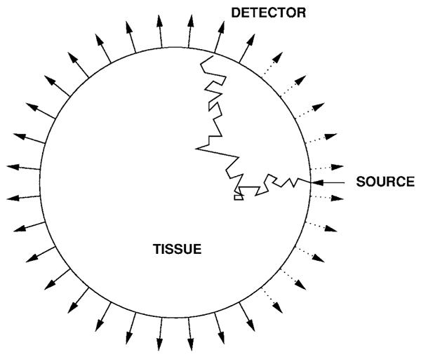
Schematic of the experimental setup. The 32 detectors and 32 sources are uniformly placed in the boundary of a circular domain with a radius of 50 mm. One source and 32 detectors are shown. The 10 detectors nearest to the source (shown with dotted lines) are not used in our calculations.

The data types are defined based on the theoretically obtained TPSF (the vectors are in bold):

$$\text{Sampled Waveform:}{\Gamma }_{\mathbf{qm}}\text{with}{\left[{\Gamma }_{qm}\right]}_i={\int }_{t_i}^{t_{i+1}}{\Gamma }_{qm}\left(t\right)\mathrm{d}t,$$ (5)

$$\text{Total Number of Photons:}{E}_{qm}={\int }_0^{\infty }{\Gamma }_{qm}\left(t\right)\mathrm{d}t,$$ (6)

$$\text{Sampled Normalized Waveform:}\mathbf{N}{\Gamma }_{\mathbf{qm}}=\frac{{10}^5}{E_{qm}}\cdot {\Gamma }_{\mathbf{qm}},$$ (7)

$$\text{Mean Time:}{\tau }_{qm}=\frac{1}{E_{qm}}{\int }_0^{\infty }t{\Gamma }_{qm}\left(t\right)\mathrm{d}t.$$ (8)

Even if we restrict ourselves to time-domain systems, other data types could be chosen.¹⁵ We chose these data types because E and τ are the first two moments of Γ(t) and NГ is the output of the MONSTIR system. Understanding the information content of these data types provides an insight into current experimental approaches.^5,6

4. SIGNAL AND BACKGROUND TYPES

We consider the detection of variations in both the attenuation (μ_a) and reduced scatter (${\mu }_s^{\prime }$) coefficients in uniform (flat) and structured (lumpy) backgrounds. Fluctuations in tissue oxygenation cause a correlated change in μ_a and ${\mu }_s^{\prime }$.¹⁶ A signal with a correlated increase in both μ_a and ${\mu }_s^{\prime }$ was considered in a previous paper.¹⁷ We begin by considering signals where μ_a or ${\mu }_s^{\prime }$ is perturbed to study how each of the parameters affects the performance of each data type. The signals were truncated Gaussians:

$${\mu }_{a,+}\left(\mathbf{r}\right)=\{\begin{array}{cc}\Delta {\mu }_{a,\max }{e}^{-\Vert \mathbf{r}-{\mathbf{r}}_o{\Vert }^2∕2s^2}\hfill & :\Vert \mathbf{r}-{\mathbf{r}}_o\Vert <3s\hfill \\ 0\hfill & :\text{otherwise}\hfill \end{array}\phantom{\}},$$ (9)

$${\mu }_{s,+}^{\prime }\left(\mathbf{r}\right)=\{\begin{array}{cc}\Delta {\mu }_{s,\max }^{\prime }{e}^{-\Vert \mathbf{r}-{\mathbf{r}}_o{\Vert }^2∕2s^2}\hfill & :\Vert \mathbf{r}-{\mathbf{r}}_o\Vert <3s\hfill \\ 0\hfill & :\text{otherwise}\hfill \end{array}\phantom{\}},$$ (10)

where μ_a,+ and ${\mu }_{s,+}^{\prime }$ are signals with increased attenuation and scatter, respectively, $\Delta {\mu }_{a,\max }$ and $\Delta {\mu }_{s,\max }^{\prime }$ are the maximum values, r is the 2D spatial coordinate, r_o is the location of the signal, and s is the width of the signal. In this paper we keep the following parameters constant: $\Delta {\mu }_{a,\max }=0.0001m{m}^{-1}$, $\Delta {\mu }_{s,\max }^{\prime }=0.01m{m}^{-1}$, and s =1.0 mm. These parameters were chosen in order to create lesions at the threshold of detectability in the raw data. While they are much fainter than we are currently able to reconstruct, they illustrate the complex dependence on location, signal type, and background.

For applications that study tissue oxygenation, changes in μ_a and ${\mu }_s^{\prime }$ are correlated, but in breast cancer imaging the changes can be anticorrelated.¹⁸ To study such tissue, we introduce a third signal type $({\mu }_{a,+},{\mu }_{s,-}^{\prime })$ where we add a μ_a,+ signal in the attenuation coefficient but subtract a $({\mu }_{a,+},{\mu }_{s,-}^{\prime })$ in the reduced scatter coefficient. From a theoretical perspective, these signals are of interest because they are similar to the set of functions comprising the null-space of E, i.e., they result in a change in the total number of photons collected that is close to zero.¹⁹

Signal detection is most often considered in a flat background. In this paper we consider flat backgrounds with μ_a=0.01 mm⁻¹ and ${\mu }_s^{\prime }$=1.0 mm⁻¹. Using a flat background is appropriate if the background fluctuations are negligible compared to the signal of interest. In practice, it is more often the case that there is background structure. To study the effect of background structure on the detection task we introduce lumpy backgrounds^9,12,20:

$$b\left(\mathbf{r}\right)=b_0+\sum _{i=1}^N\mathrm{lump}(\mathbf{r}-{\mathbf{r}}_i),$$ (11)

where b(r) is the lumpy background, b₀ is the spatial mean (equal to flat background value), N is the Poisson-distributed number of lumps and r_i is the uniformly distributed location of each lump (with an equal probability of being placed anywhere in the domain). The lumps have the following form:

$$\mathrm{lump}(\mathbf{r}-{\mathbf{r}}_i)=l_0{e}^{-\Vert \mathbf{r}-{\mathbf{r}}_i{\Vert }^2∕2w^2}-\frac{1}{A\left(\Omega \right)}{\int }_{\Omega }{l}_0{e}^{-\Vert \mathbf{r}-{\mathbf{r}}_i{\Vert }^2∕2w^2}{\mathrm{d}}^{2}r,$$ (12)

where l_o is the lump strength, w is the lump width, Ω is the domain (in our case a disk), and A(Ω) is the area of the domain. The second term in the expression for the lumps was designed such that the ensemble mean of the lumpy background is the flat background. We consider lumps in the attenuation coefficient. They are similar to the μ_a,+ signals but with different amplitudes and widths, w=4 mm, $\stackrel{‒}{N}=2000$, and $l_o=0.1\cdot \Delta {\mu }_{a,\max }$. Figure 2 shows a sample lumpy background and signal.

Fig. 2.

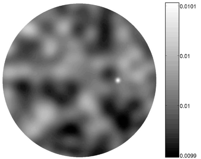
Sample lumpy background (in μ_a [mm⁻¹]) and signal half way from the center to the boundary of the domain. The correlated structure of the background confounds the task of detecting the signal.

5. INFORMATION CONTENT: A DETECTION-THEORETIC VIEW

We quantify the information of a data set from the perspective of statistical detection theory. The task is to detect a signal in the parameter of interest from the measurements. This implies discriminating between the following two hypotheses:

$$\begin{array}{cc}\hfill {\mathbf{g}}_0& =\langle \mathbf{g}\left(b\right)\rangle +\mathbf{n}\text{if the signal is absent,}\hfill \\ \hfill {\mathbf{g}}_i& =\langle \mathbf{g}(b+s)\rangle +\mathbf{n}\text{if the signal is present,}\hfill \end{array}$$ (13)

where g_i are the measurements under the ith hypothesis, $\langle g\left(b\right)\rangle$ is the noise-free data (averaged both over measurement noise and random backgrounds) from the backgrounds, $\langle g(b+s)\rangle$ is the noise-free data from the backgrounds and signals, and n is the noise. The noise term will include both the randomness due to the Poisson nature of photon counting and the uncertainty due to background variation.

To quantify the ability to detect signals from the data, we use the ideal linear (Hotelling) observer^9,12:

$$t_{\mathrm{Hot}}\left(\mathbf{g}\right)=\Delta {\mathbf{g}}^t{\mathbf{K}}_{\mathtt{g}}^{-1}\mathbf{g},$$ (14)

where

$$\Delta \mathbf{g}=\langle \mathbf{g}(b+s)\rangle -\langle \mathbf{g}\left(b\right)\rangle ,$$ (15)

and ${\mathbf{K}}_g^{-1}$ is the inverse of the data covariance matrix. Note that since the imaging system is nonlinear, in general ⟨g(s)⟩ ≠ ⟨g(b+s)⟩−⟨g(b)⟩.

The Hotelling observer maximizes the signal-to-noise ratio (SNR_t) among all linear test statistics¹¹ with

$${\mathrm{SNR}}_t=\frac{\langle t_1\rangle -\langle t_0\rangle }{\sigma \left(t\right)},$$ (16)

where $\langle t_i\rangle$ is the ensemble average under the ith hypothesis, and σ(t) is the standard deviation of the test statistic (assumed to be the same under both hypotheses owing to the low contrast signal used). The SNR² for the Hotelling observer $\left({\mathrm{SNR}}_{\mathrm{Hot}}^2\right)$ is given by

$${\mathrm{SNR}}_{\mathrm{Hot}}^2=\Delta {\mathbf{g}}^t{\mathbf{K}}_{\mathtt{g}}^{-1}\Delta \mathbf{g}.$$ (17)

If the test statistic is Gaussian, the Hotelling observer also maximizes the area under the receiver operating characteristic (ROC) curve.^11,12 For a discussion of making the Gaussian assumption in this application see Appendix A.

6. NOISE MODELS

For ${\mathrm{SNR}}_{\mathrm{Hot}}^2$ computations, we need to compute the data covariance matrix for each of the data types. The noise model for our data types assumes we have the output of MONSTIR and some independent measurement of E. The analysis is intended to examine how much would be gained by adding the information from the total number of photons collected. For a fixed background, we assume the dominant noise in the normalized waveform to be Poisson, hence NΓ for a fixed background is a Poisson random vector.² We consider estimating the mean time from the noisy normalized waveform:

$$\tau ={\int }_0^{\infty }t\left[\frac{N\Gamma \left(t\right)}{{\int }_0^{\infty }N\Gamma \left(t\right)\mathrm{d}t}\right]\mathrm{d}t.$$ (18)

In the limit of a large mean number of arriving photons N_a (10⁵ in our case) at a given detector, the variance of τ, based on the diffusion approximation model, is given by²¹

$${\sigma }_{\tau }^2=\frac{1}{N_a}\left\{{\int }_0^{\infty }{t}^2\left[\frac{\stackrel{‒}{N\Gamma }\left(t\right)}{{\int }_0^{\infty }\stackrel{‒}{N\Gamma }\left(t\right)\mathrm{d}t}\right]\mathrm{d}t-{\stackrel{‒}{\tau }}^2\right\}.$$ (19)

The measurements of E are assumed to be Poisson with the variance equal to 10⁵ arriving photons. For the full waveform computations, we assume NΓ and E are independent Poisson measurements and combine them. If both of these data types were measured from the same waveform, they would not be independent. The implication of this assumption is that there are two measurement systems, one that measures E and another that measures NΓ.

7. MONTE CARLO ESTIMATE OF ${\mathrm{SNR}}_{\mathrm{Hot}}^2$ WITH RANDOM BACKGROUNDS

In a flat background, the noise is independent for every source—detector combination, therefore the covariance matrix due to measurement noise is diagonal. Structured backgrounds introduce correlations between measurements from different source—detector pairs. For these backgrounds the covariance matrix has a component that arises from the photon measurement noise and one that arises from the background variation⁹:

$${\mathbf{K}}_{\mathtt{g}}=\langle {\mathbf{K}}_{\mathtt{g},\text{meas}}{\rangle }_b+{\mathbf{K}}_{\mathtt{g},\mathrm{lumps}},$$ (20)

where K_g,meas is the measurement covariance matrix for a fixed background, $\langle \cdot \rangle b$ is the ensemble mean over backgrounds, and K_g,lumps the lumpy background component of the covariance matrix

$${\mathbf{K}}_{\mathtt{g},\mathrm{lumps}}=\langle (\stackrel{‒}{\mathbf{g}}-\overline{\stackrel{‒}{\mathbf{g}}}){(\stackrel{‒}{\mathbf{g}}-\overline{\stackrel{‒}{\mathbf{g}}})}^t{\rangle }_b,$$ (21)

with $\stackrel{‒}{g}=\langle g{\rangle }_{n\mid b}$ (the mean over the measurement noise for a fixed background) and $\overline{\stackrel{‒}{g}}=\langle \langle g{\rangle }_{n\mid b}{\rangle }_b$ (the mean over both the measurement noise and random backgrounds).

The lumps introduce spatial correlations in the backgrounds that result in correlations in the data. One of the goals of this research was to study the robustness of the data types to these correlations. To estimate ${\mathrm{SNR}}_{\mathrm{Hot}}^2$ for the lumpy background case we generate noise-free samples of the data $\left\{\stackrel{‒}{g}\right\}$ (for individual realizations of the lumpy background). From these samples we estimate ${\mathrm{SNR}}_{\mathrm{Hot}}^2$ as a function of sample size N by estimating the mean data over the ensemble of backgrounds,

$$\widehat{\overline{\stackrel{‒}{\mathbf{g}}}}\left(N\right)=\frac{1}{N}\sum _{i=1}^N{\stackrel{‒}{\mathbf{g}}}_i,$$ (22)

the mean signal data,

$$\widehat{\overline{\stackrel{‒}{\Delta \mathbf{g}}}}\left(N\right)=\frac{1}{N}\sum _{i=1}^N{\stackrel{‒}{\Delta \mathbf{g}}}_i,$$ (23)

the covariance matrix,

$${\widehat{\mathbf{K}}}_{\mathtt{g}}\left(N\right)=\frac{1}{N}\sum _{i=1}^N{K}_{\mathtt{g},\text{meas}}\left(i\right)+\frac{1}{N-1}\sum _{i=1}^N({\stackrel{‒}{\mathbf{g}}}_i-\widehat{\overline{\stackrel{‒}{\mathbf{g}}}}\left(N\right)){({\stackrel{‒}{\mathbf{g}}}_i-\widehat{\overline{\stackrel{‒}{\mathbf{g}}}}\left(N\right))}^t,$$ (24)

and using them to estimate ${\mathrm{SNR}}_{\mathrm{Hot}}^2$:

$${\mathrm{SNR}}_{\mathrm{Hot}}^2\left(N\right)=\widehat{\overline{\stackrel{‒}{\Delta {\mathbf{g}}^t}}}{\widehat{\mathbf{K}}}_{\mathtt{g}}^{-1}\widehat{\overline{\stackrel{‒}{\Delta \mathbf{g}}}}.$$ (25)

8. RESULTS AND DISCUSSION

We begin by examining the detectability $\left({\mathrm{SNR}}_{\mathrm{Hot}}^2\right)$ of signals in a flat background as a function of depth. All plots stop 5 mm from the boundary because of the signal size and the limits of the diffusion model near the boundary. A spatial detectability map for the μ_a,+ lesion and E shows that due to symmetry there is little angular dependence to the detectability at these depths (Fig. 3), so further results focus on the detectability along the (x,0) line (from center to a source).

Fig. 3.

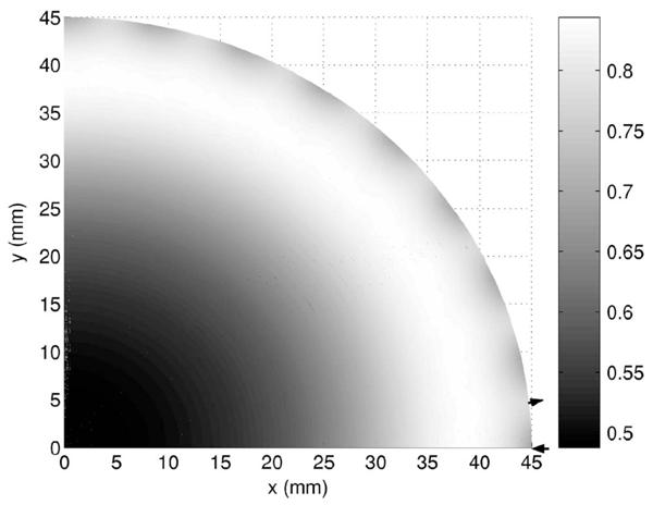
Detectability of μ_a,+ signal in a flat background showing only a small angular dependence away from the boundary. The maxima in the boundary occur near the detectors. The arrow pointing into the domain shows the location of one of the sources, and the arrow pointing outward shows the location of a detector. As expected, the detectability is lower in the center of the domain.

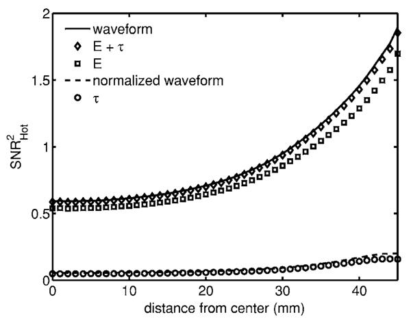
Figure 4 shows the detectability of a μ_a,+ signal in a flat background. The majority of the information of the waveform is contained by E, and the maximum detectability occurs away from the boundary. In this situation, the normalized waveform can be summarized by τ with little loss of information. It is also interesting to see that the full waveform can be summarized by the first two moments with little or no information loss.

Fig. 4.

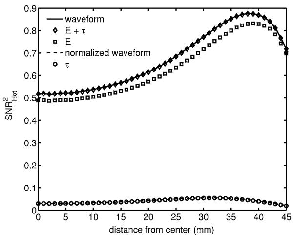
Detectability of μ_a,+ signal1 in a flat background. Note that the normalized waveform and τ plots overlap. For an attenuating inclusion in a flat background, the majority of the information is encoded by the total counts. Peak detectability occurs close to the boundary.

The figure for the ${\mu }_{s,+}^{\prime }$ lesion (Fig. 5) behaves differently. The maximum detectability occurs as the signal approaches the boundary, τ does not encode all the information of the normalized waveform, and there are differences close to the boundary. For the ${\mu }_{a,+},{\mu }_{s,-}^{\prime }$ signal (Fig. 6), E, τ, and the normalized waveform have comparable information close to the boundary, but as the signal gets deeper in the tissue, E loses its information content faster than the other two data types.

Fig. 5.

Detectability of ${\mu }_{s,-}^{\prime }$ signal in a flat background. For a scattering inclusion the total counts contain the majority of the information, and peak detectability occurs at the boundary.

Fig. 6.

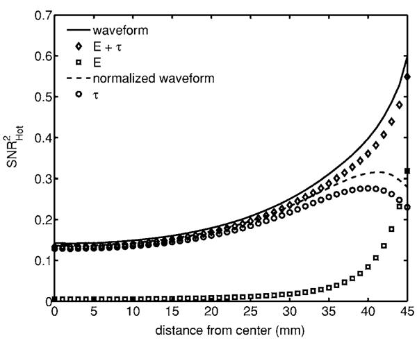
Detectability of ${\mu }_{a,+},{\mu }_{s,-}^{\prime }$ signal in a flat background. For an inclusion that has an increase in attenuation and scatter, the mean time contains most of the information, and we see that the behavior near the boundary depends on the data type.

In both of the previous results, signals near the boundary produce larger changes in the data. Given the illposedness of the reconstruction problem, solutions would be biased to contain more structure near the boundary. Spatially varying regularization^22–24 reduces this bias by regularizing the reconstructions more at the boundary than at the center. The work presented here could be used to provide a detection-theoretic basis for generating reconstructions that regularized both μ_a and μ_s depending on their respective spatial detectability.

Throughout this paper we have not used the data from the five nearest detectors on either side of each source. We consider how much would be gained if the electronics allowed us to collect data from the excluded detectors. Using a μ_a,+ signal and a flat background, Fig. 7 shows that near the boundary there is a significant gain in information but not so much near the interior. While our analysis has been tailored for the MONSTIR system, the approach is generic as is the qualitative behavior.

Fig. 7.

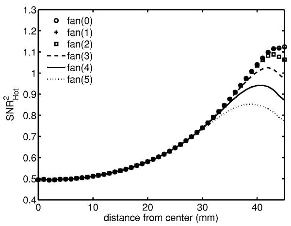
Detectability for μ_a,+ lesion and the E data type in a flat background. Each curve represents exclusion of a different number of detectors at either side of each source. Note that using all detectors [fan(0)] and only excluding one [fan(1)] produces plots that lie on top of each other.

The degree to which the anatomical fluctuations will affect the detectability of a particular signal will depend on how much the lumps resemble the signal in the data. Figure 8 shows the convergence plot for ${\mathrm{SNR}}_{\mathrm{Hot}}^2\left(N\right)$ with four independent samples of 500 lumpy backgrounds each and μ_a,+ lesion. For a finite number of samples, ${\mathrm{SNR}}_{\mathrm{Hot}}^2\left(N\right)$ is biased high as an estimate of the SNR² for the entire ensemble.

Fig. 8.

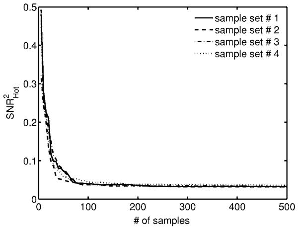
Stability plot for four sets of 500 lumpy backgrounds each. We see that for the random backgrounds our detectability estimate is biased high for a small number of samples but converges as we increase our sample size.

As an example of the effect of anatomical variation we include a μ_a,+ signal in the lumpy background (Fig. 9). The behavior of E near the boundary with lumpy backgrounds differs from the behavior in the flat background plot (Fig. 4). For the lumpy background the detectability continues to increase as the signal gets closer to the boundary. The background variations also increase the rate at which the information decreases for E as the signal gets deeper in the tissue. There is an overall decrease in information for both data types since the lumps add uncertainty in the data. It seems that E loses more information because of the lumps than does τ, i.e., it is less robust to background fluctuations. To quantify this statement we averaged ${\mathrm{SNR}}_{\mathrm{Hot}}^2$ over the signal locations

$$\langle {\mathrm{SNR}}_{\mathrm{Hot}}^2{\rangle }_{\mathrm{loc}}=\frac{1}{N}\sum _{i=1}^N{\mathrm{SNR}}_{\mathrm{Hot}}^2\left(l_i\right),$$ (26)

where N is the number of lesions and SNR²_Hot(l_i) is the detectability of a lesion located at location l_i. For E, $\langle {\mathrm{SNR}}_{\mathrm{Hot}}^2{\rangle }_{\mathrm{loc}}\left(lumpy\right)=0.09\langle {\mathrm{SNR}}_{\mathrm{Hot}}^2{\rangle }_{\mathrm{loc}}\left(flat\right)$, where for τ, $\langle {\mathrm{SNR}}_{\mathrm{Hot}}^2{\rangle }_{\mathrm{loc}}\left(lumpy\right)=0.32\langle {\mathrm{SNR}}_{\mathrm{Hot}}^2{\rangle }_{\mathrm{loc}}\left(flat\right)$. This suggests that for this combination of data type and anatomical variation, the mean time has more robustness to anatomical variation than the total counts. This kind of statistical robustness of certain data types to random backgrounds has also been explored in the context of time-reversal imaging.²⁵

Fig. 9.

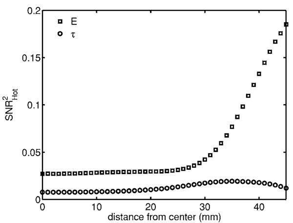
Detectability of μ_a,+ signal in a lumpy background. The randomness in the background reduces the detectability of the inclusions and affects the behavior close to the boundary. We see that the mean time has a lower but more uniform detectability than the total counts in the presence of random fluctuations in the background. The overall decrease in detectability for the mean time was less than that for the total counts when compared to the flat background.

To take the analysis of the anatomical variation further would require a characterization of the statistics of the backgrounds²⁶ and signals. Our result on the robustness of the data type is dependent on the data type and background. If the background were to vary with lumps similar to the ${\mu }_{a,+},{\mu }_{s,-}^{\prime }$ lesion, the mean time would be more affected than the total counts. Such a characterization possibly obtained by using a database of optical tomography images would allow the incorporation of the anatomical fluctuations into the analysis in a quantitative way that would allow analysis applicable to specific systems. In this paper we have considered the correlations in the data caused by the lumpy background, but such correlations can also be caused by modeling error.^27,28

For the lumpy background results we exclude the waveform and normalized waveform because of the computational resources required. The waveform data sets are 1024 (source—detector pairs) ×300 (time samples). The covariance matrix for such a data set would have (1024×300)² elements. It might be possible to use a sparse representation under approximations regarding the amount of correlation between detectors or a different dimensionality reduction. Such an analysis lies beyond the scope of this paper but there are several approaches that can be used for handling large matrices.^12,29

The map from the optical parameters to the data is nonlinear. The nonlinearity presents a challenge in generalizing the results presented in this paper. Much as the exact form of the photon measurement density functions depends on the background value³⁰ so will the spatial detectability maps. While the exact shape will vary, the general patterns are likely to remain the same.

9. CONCLUSIONS

The information content of each data type depends on the type of signal, the location of the signal, and the type of background. For a flat background and μ_a,+ or ${\mu }_s,\prime$ signals, E contains most of the information in the waveform. For the ${\mu }_{a,+},{\mu }_{s,-}^{\prime }$ signal, τ contains more than E. We also see that a combination of E and τ summarizes most of the information content of the entire waveform.

The effect of the background variation on the data types is correlated with how similar the lump is to the signal in that data space. The location averaged detectability quantifies that effect. For the case presented, the mean time is more robust to anatomical fluctuations than the total number of counts. In general, the result will depend on the combination of background and the signal being detected.

We have established a methodology for evaluating the information content of data types for optical tomography as a nonlinear system using spatial detectability plots and Monte Carlo methods.

APPENDIX A: MAKING THE GAUSSIAN ASSUMPTION

The Hotelling observer maximizes SNR_t among all linear observers. If the test statistic t is Gaussian then there is a monotonic transformation between SNR_t and the area under the receiver operating characteristic (AUC) curve¹¹,¹²:

$${\mathrm{AUC}}_G\left({\mathrm{SNR}}_t\right)=\frac{1}{2}+\frac{1}{2}\mathrm{erf}\left(\frac{{\mathrm{SNR}}_t}{2}\right),$$ (A1)

where erf(·) is the error function. The AUC can be interpreted as the average fraction, correct when making the decision of whether the lesion is present. Figure 10 shows a standardized histogram (with N=2000 samples) of t_Hot with a μ_a,+ signal and lumpy background for the E data type. The histogram appears Gaussian, but we check the validity of Eq. (A1) by comparing it to the AUC obtained by using the Mann—Whitney U-statistic³¹:

$${\mathrm{AUC}}_{\mathrm{MW}}=\frac{1}{N^2}\sum _{i=1}^N\sum _{j=1}^N\text{step}(t_j^1-t_i^0),$$ (A2)

where $t_j^1$ is the value of the test statistic on the jth background with the signal present and $t_i^0$ value of the test statistic on the ith background with the signal absent. We obtained AUC_G=0.55 and AUC_MW=0.56. It seems that for this application, SNR_Hot can be interpreted as a monotonic transformation of AUC.

Fig. 10.

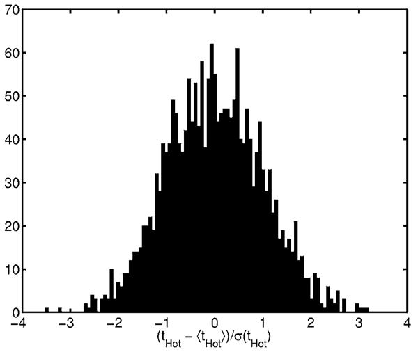
Histogram of standardized Hotelling test statistic. The approximate Gaussianity of the test statistic justifies using ${\mathrm{SNR}}_{\mathrm{Hot}}^2$ as our measure of detectability.

REFERENCES

- 1.Gibson AP, Hebden JC, Arridge SR. Recent advances in diffuse optical tomography. Phys. Med. Biol. 2005;50:R1–R43. doi: 10.1088/0031-9155/50/4/r01. [DOI] [PubMed] [Google Scholar]
- 2.Schmidt FEW, Fry ME, Hillman EMC, Hebden JC, Delpy DT. A 32-channel time-resolved instrument for medical optical tomography. Rev. Sci. Instrum. 2000;71:256–265. [Google Scholar]
- 3.Pogue BW, Testorf M, McBride T, Osterberg U, Paulsen K. Instrumentation and design of a frequency-domain diffuse optical tomography imager for breast cancer detection. Opt. Express. 1997;1:391–403. doi: 10.1364/oe.1.000391. [DOI] [PubMed] [Google Scholar]
- 4.Schweiger M, Gibson AP, Arridge SR. Computational aspects of diffuse optical tomography. IEEE Comput. Sci. Eng. 2003;5:33–41. [Google Scholar]
- 5.Hebden JC, Arridge SR, Delpy DT. Optical imaging in medicine: I. Experimental techniques. Phys. Med. Biol. 1997;42:825–840. doi: 10.1088/0031-9155/42/5/007. [DOI] [PubMed] [Google Scholar]
- 6.Arridge SR. Optical tomography in medical imaging. Inverse Probl. 1999;15:R41–R93. [Google Scholar]
- 7.Pogue BW, Willscher C, McBride TO, Österberg UL, Paulsen KD. Contrast-detail analysis for detection and characterization with near-infrared diffuse tomography. Med. Phys. 1995;22:1779–1792. doi: 10.1118/1.1323984. [DOI] [PubMed] [Google Scholar]
- 8.Boas DA, O’Leary MA, Chance B, Yodh AG. Detection and characterization of optical inhomogeneities with diffuse photon density wave: a signal-to-noise analysis. Appl. Opt. 1997;36:75–92. doi: 10.1364/ao.36.000075. [DOI] [PubMed] [Google Scholar]
- 9.Barrett HH. Objective assessment of image quality: effects of quantum noise and object variability. J. Opt. Soc. Am. A. 1990;7:1266–1278. doi: 10.1364/josaa.7.001266. [DOI] [PubMed] [Google Scholar]
- 10.Barrett HH, Abbey CK, Clarkson E. Objective assessment of image quality. II. Fisher information, Fourier crosstalk, and figures of merit for task performance. J. Opt. Soc. Am. A. 1995;12:834–852. doi: 10.1364/josaa.12.000834. [DOI] [PubMed] [Google Scholar]
- 11.Barrett HH, Abbey CK, Clarkson E. Objective assessment of image quality. III. ROC metrics, ideal observers, and likelihood-generating functions. J. Opt. Soc. Am. A. 1998;15:1520–1535. doi: 10.1364/josaa.15.001520. [DOI] [PubMed] [Google Scholar]
- 12.Barrett HH, Myers KJ. Foundations of Image Science. Wiley; 2004. [Google Scholar]
- 13.Schweiger M, Arridge SR, Hiraoka M, Delpy DT. The finite element method for the propagation of light in scattering media: Boundary and source conditions. Med. Phys. 1995;22:1779–1792. doi: 10.1118/1.597634. [DOI] [PubMed] [Google Scholar]
- 14.Arridge SR, Schweiger M, Hiraoka M, Delpy DT. A finite element approach to modeling photon transport in tissue. Med. Phys. 1993;20:299–309. doi: 10.1118/1.597069. [DOI] [PubMed] [Google Scholar]
- 15.Schweiger M, Arridge SR.Optimal data types in optical tomography 1997123071–84.Proceedings of the 15th Conference on Information Processing in Medical Imaging, Lecture Notes in Computer Science, Springer [Google Scholar]
- 16.Gerken M, Faris GW. Frequency-domain immersion technique for accurate optical property measurements of turbid media. Opt. Lett. 1999;24:1726–1728. doi: 10.1364/ol.24.001726. [DOI] [PubMed] [Google Scholar]
- 17.Pineda AR, Barrett HH, Arridge SR. Spatially varying detectability for optical tomography. Proc. SPIE. 2000;3977:77–83. [Google Scholar]
- 18.Tromberg BJ, Coquoz O, Fishkin JB, Pham T, Anderson ER, Butler J, Cahn M, Gross JD, Venugopalan V, Pham D.Non-invasive measurements of breast tissue optical properties using frequency-domain photon migration Philos. Trans. R. Soc. London 1997, Ser. B 352661–668. [DOI] [PMC free article] [PubMed] [Google Scholar]
- 19.Arridge SR, Lionheart WRB. Nonuniqueness in diffusion-based optical tomography. Opt. Lett. 1998;23:882–884. doi: 10.1364/ol.23.000882. [DOI] [PubMed] [Google Scholar]
- 20.Myers KJ, Rolland JP, Barrett HH, Wagner RF. Aperture optimization for emission imaging: effect of a spatially varying background. J. Opt. Soc. Am. A. 1990;7:1279–1293. doi: 10.1364/josaa.7.001279. [DOI] [PubMed] [Google Scholar]
- 21.Arridge SR, Hiraoka M, Schweiger M. Statistical basis for the determination of optical path length in tissue. Phys. Med. Biol. 1995;40:1539–1558. doi: 10.1088/0031-9155/40/9/011. [DOI] [PubMed] [Google Scholar]
- 22.Arridge SR, Schweiger M.Inverse methods for optical tomography 1997687259–277.Proceedings of the 13th Conference on Information Processing in Medical Imaging, Lecture Notes in Computer Science, Springer [Google Scholar]
- 23.Pogue BW, McBride TO, Prewitt J, Osterberg UL, Paulsen KD. Spatially variant regularization improves diffuse optical tomography. Appl. Opt. 1999;38:2950–2961. doi: 10.1364/ao.38.002950. [DOI] [PubMed] [Google Scholar]
- 24.Zhou J, Bai J, He P. Spatial location weighted optimization scheme for DC optical tomography. Opt. Express. 2003;11:141–149. doi: 10.1364/oe.11.000141. [DOI] [PubMed] [Google Scholar]
- 25.Bal G, Pinaud O. Time-reversal-based detection in random media. Inverse Probl. 2005;21:1593–1619. [Google Scholar]
- 26.Kupinski MA, Clarkson E, Hoppin JW, Chen L, Barrett HH. Experimental determination of object statistics from noisy images. J. Opt. Soc. Am. A. 2003;20:421–429. doi: 10.1364/josaa.20.000421. [DOI] [PMC free article] [PubMed] [Google Scholar]
- 27.Kaipio J, Somersalo E. Statistical and Computational Inverse Problems. Springer; 2005. [Google Scholar]
- 28.Arridge SR, Kaipio JP, Kolehmainen V, Schweiger M, Somersalo E, Tarvainen T, Vauhkonen M. Approximation errors and model reduction with an application in optical diffusion tomography. Inverse Probl. 2006;22:175–195. doi: 10.1109/IEMBS.2006.260738. [DOI] [PubMed] [Google Scholar]
- 29.Barrett HH, Myers KJ, Gallas B, Clarkson E, Zhang H. Megalopinakophobia: its symptoms and cures. Proc. SPIE. 2001;4320:299–307. [Google Scholar]
- 30.Arridge SR, Schweiger M. Photon-measurement density-functions. Part 2. Finite-element-method calculations. Appl. Opt. 1995;34:8026–8037. doi: 10.1364/AO.34.008026. [DOI] [PubMed] [Google Scholar]
- 31.Swets JA, Pickett RM. Evaluation of Diagnostic Systems: Methods from Signal Detection Theory. Academic; 1982. [Google Scholar]