For prediction of elder survival by a Gompertz model, number dead is preferable to number alive

Abstract

The standard Gompertz equation for human survival fits very poorly the survival data of the very old (age 85 and above), who appear to survive better than predicted. An alternative Gompertz model based on the number of individuals who have died, rather than the number that are alive, at each age, tracks the data more accurately. The alternative model is based on the same differential equation as in the usual Gompertz model. The standard model describes the accelerated exponential decay of the number alive, whereas the alternative, heretofore unutilized model describes the decelerated exponential growth of the number dead. The alternative model is complementary to the standard and, together, the two Gompertz formulations allow accurate prediction of survival of the older as well as the younger mature members of the population.

Introduction

According to the Gompertz (1825) “law,” the number of individuals alive in a human population decreases exponentially with age at an exponentially increasing rate. As Gompertz and many others have pointed out, that model serves well only for persons between about 25 and 85 years of age. The discrepancy outside that age range is not evident in the ordinary survival plot but is obvious in plots of mortality rate against age. In their survey, Olshansky and Carnes (1997) consider extensively “non-Gompertzian mortality at older ages”. The older members of the population depart erratically from the classical model but overall survival is better than predicted by the standard Gompertz “law.” Here we demonstrate that elder survival is accurately predicted by an alternative Gompertz equation, which tracks the number dead.

The small, but growing, 85 and older population has attracted particular attention (Riggs and Millecchia 1992; Robine and Vaupel 2001). As the size of this population has expanded, the statistical fluctuation of mortality rates in extreme old age has increased, and the failure of the standard Gompertz model has become more obvious and more important. Empirically selected smoothing functions (Faber 2001) have been generated for life tables, but unsmoothed life tables (Depoid 1972; Barrett 1985; Riggs and Millecchia 1992; Robine and Vaupel 2001) continue to display considerable fluctuation or “noise” that obscures the underlying form of the function. The alternative formulation of the Gompertz model described here provides a “smooth” prediction of elder survival.

The characteristic form of the alternative, compared to that of the standard, Gompertz survival functions, is illustrated in Fig. 1. The human survival curve (H in Fig. 1, data from Statistical Abstracts of Sweden 1991) is of the well-known standard Gompertz form, with a wide early shoulder and steeper termination. The Mediterranean fruit-fly curve (F in Fig. 1) (Carey et al. 1992; Easton 1995, 1997) has the alternative shape and is fit by the alternative model. In contrast to the standard, the alternative survival curve descends early and terminates with a slow decline.

Fig. 1.

Exemplary patterns of survival. F Alternative Gompertz survival model: Points relative number of Mediterranean fruit flies still alive after Day 0 (Carey et al. 1992). Line F; Eq. 5b fit to data F (death rate, Eq. 4b, decreases exponentially). Parameters: b = 10.532, k = 0.139, . H Standard Gompertz survival model: Points relative number of persons alive at each age after Year 0 (Statistical Abstracts of Sweden 1991). Line H; Eq. 3 fit to data H (mortality rate, Eq. 2b, increases exponentially). Parameters: b = 0.00007, k = 0.11, n_o = 98

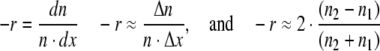
In the standard view, survival is expressed in terms of proportional decrease in number alive per year. That measure is variously called probability of death, force of mortality, hazard rate, failure rate, and instantaneous mortality rate (Gavrilov and Gavrilova 1991). Here we retain the term “mortality rate” to designate the standard survival rate. The alternative model is based on the proportional increase in the number that have died in a population, and we therefore appropriate the term “death rate” (Eq. 4b) to designate the alternative survival rate. This “death rate” does not replace but rather supplements the conventional standard “mortality rate” (Eq. 2b),

The striking success of the “number dead” model in predicting survival of cohorts of fruit flies and other animals (Easton 1995, 1997) raises the question whether the “elder discrepancy” in the human Gompertz survival prediction might be accounted for in a similar way.

Because it is a generally unfamiliar concept, the number dead model is here compared directly with the standard survival equation. Further details of the derivations are available elsewhere (Easton 1995). The functional notation is more convenient and less cumbersome for mathematical manipulations than is the subscript notation used in standard life tables. The two systems of notation are compared in Table 1.

Table 1.

Comparison of functional notation (for the standard and alternative models) with life-table notation

Quantity	Functional notation		Life-table notation
Age	x		x
Number of survivors	n(x)		lx
Total population size	N∞	no	lo
Number dying in one year	−ΔN	Δn	dx
Probability of death	R	r	qx

The Gompertz (1825) survival function, expressed in modern notation (Batschelet 1971), is a special case of the general differential equation:

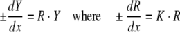1a,b

In the following, lower-case symbols refer to the standard Gompertz model, upper case to the alternative model.

Standard Gompertz model

When dY/dx is negative and dR/dx positive, the solution of Eq. 1 is the classical, standard Gompertz survival curve for humans. Therefore, in Eq. 1, Y = n, the number alive (survivors) in the population, decreases at mortality rate r, and Eq. 1 then takes the form:

2a,b

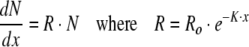
Substitute Eq. 2b into Eq. 2a and integrate the result between the initial population, n_o, at age x = 0, and the population n, at age x; then the standard Gompertz survival equation (Fig. 1, curve H) is:

3

where b = r_o/k and the total initial live population is n_o. Note positive , i.e., r increases with age

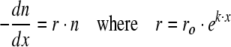
Alternative Gompertz model

When, in Eq. 1, dY/dx is positive and dR/dx is negative, the solution is the Gompertz growth curve. In that instance, the number dead, N, increases exponentially at rate R:

4a,b

The proportionality coefficient, R, is here defined as the death rate, the rate of increase in number dead, at rate K. Rate R decreases with age.

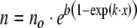
Substitute Eq. 4b into Eq. 4a, rearrange and integrate the result between N, x, and the final total dead population, , as x → ∞; then:

5a,b

Where, in B = R_o/K, parameter N is the cumulative number dead by age x, R is the death rate, and n is the number still alive by age x. Note negative . Equation 5b describes survival according to the alternative Gompertz survival equation. For a particular data set, the total number dead, , the original total number alive.

Although based on the same equation, the survival functions defined by r and R are different, because the former concerns the accelerated decrease from a large number of live individuals, whereas the latter is based on the decelerated increase from a very small number dead.

Methods

Study populations

Carey et al. (1992, Table 2) provide a chart of the number of Medflies alive each day, starting from an original population of 1,203,646. Those numbers provide the points in survival curve F, Fig. 1. Precision (computer) fitting of the alternative Gompertz equation (Eq. 5) to these points was accomplished by a least-squares minimization procedure used for nonlinear equations in the program “Scientist” (Micromath) (F, Fig. 1). The same procedure was used to fit the standard Gompertz equation (Eq. 3) to the human survival data (H, Fig. 1). Those data, taken from conventional life tables (Statistical Abstracts of Sweden 1991), consist of the estimated number of survivors each year out of an original 100,000 individuals. With only two rate constants in each, the equations are sufficiently simple that a curve fit visually indistinguishable from the machine result can be easily obtained by successive manual adjustment of parameters.

The population critical to this discussion, i.e., humans (males) older than 85 years, is taken from Table I in Riggs and Millecchia (1992) (R and M), gleaned from “published federal government sources” (National Center for Health Statistics; http://www.cdc.gov/nchs/). The list constitutes essentially a frequency distribution of the number of deaths occurring at each age, 85–124 years, at any time during the interval 1956–1987. Deaths reported for ages 125 and above were lumped as one group. R and M estimate an error of the order of 0.2% in these values.

At any particular age, the number of individuals alive at and above a particular age is the sum of all those who subsequently die. Based on this observation, R and M used a “cumulative summation technique” to construct the survival profile. Backward integration of the number dead data, by means of the integration option in MATHCAD, gave us the same result, which is the tail-end of a total standard survival curve. An estimate of the total population from which the oldsters were drawn, was obtained by directing the computer to find the parameters of that putative curve.

Rate calculations

The survival rate in terms of number alive, r, or in terms of number dead, R, can be calculated for any age along the survival data plot, whether the data as a whole follow the typical standard or the alternative (or any other) form. Prediction of the full range of the human survival plot requires the use of both functions.

To calculate the mortality rate from the survival data, rearrange Eq. 2a:

6a–c

where Δx = 1 (year)

Similarly, for the death rate, with Eq. 4a:

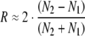7

N₁, N₂ (successive cumulative number dead by age x) and n₁, n₂ (successively diminished total number alive by age x) are sequential points along the survival data plot, as, for example, in Fig. 2.

Fig. 2.

Calculation of survival rates. Heavy line Arbitrary survival profile. If considered to be the standard Gompertz survival model (Eq. 3), the line tracks the number of individuals alive (n). Mortality rates, r(data), are calculated (Eq. 6c) from the difference between successive points divided by average number alive between those points (Eq. 6c). Representing the alternative Gompertz survival model, the line tracks the number of individuals dead (N). Death rates, R(data), are calculated from the difference between successive points divided by average number dead between those points (Eq. 7)

Results

Figure 3 shows mortality rates calculated from the Mediterranean fruit fly (Carey et al. 1992) data and also from the human data (see Fig. 1). In Fig. 4, the death rates (Eq. 7) for the same data are presented.

Fig. 3.

Calculated and theoretical mortality rates (r). Filled circles Mortality rates, r, the annual (lower scale) proportional decrease in the number of live individuals, calculated from human survival data (H in Fig. 1). Line Theoretical mortality rates determined during fit of standard equation, Eq. 3, to human survival data, H in Fig. 1. Open circles Mortality rates, r, proportional decrease in number of live flies each day (Eq. 6c), calculated from fly survival data (line F, Fig. 2) (upper scale)

Fig. 4.

Calculated and theoretical death rates (R). H, filled circles (lower scale), death rates, R, the proportional increase in number of dead individuals each year, calculated (Eq. 7) from human survival data (H in Fig. 1). F, open circles (upper scale), death rates calculated (Eq. 7) from fly survival data (F in Fig. 1). Line Theoretical death rates determined during fit of alternative equation, Eq. 7a, to fly survival data, F in Fig. 1

In Fig. 3, the calculated standard mortality rate, r, for humans, H, departs from the exponentially increasing theoretical line (Eq. 3) beyond about age 100 years. On the other hand (Fig. 4), the theoretical exponentially decreasing alternative death rate, R, for the fly (line F) conforms well to the locus of points calculated from the survival data of mature and older age individuals. The standard mortality rate, r, of the flies initially rises smoothly (F in Fig. 3a), and like the human data (H in Fig. 3a), it becomes erratic at older ages; the alternative death rates, R, of the fly and of the human elders both terminate smoothly (F and H in Fig. 4).

Application of the alternative function specifically to data for ages 85–124

The total survival curve, of which the elder group is the tail end, was specified by b, k, and n_o, obtained by machine fitting Eq. 3 to the calculated elder survival data. Thus n_o, the initial population, was estimated at about 39 million, approximately the US human male population of the early twentieth century. This estimated n_o was used in the calculation of the mortality rates and the death rates of the elder population. In logarithmic plot Fig. 5, both predictions follow nearly straight lines from 85 to almost 100 years of age. At greater age, the logarithmic standard mortality rate diverges dramatically, but the logarithmic alternative death rate continues along a nearly smooth monotonic trajectory. A similar trajectory is obtained from a plot of the logarithm of number of survivors vs age categories (Fig. 5, inset).

Fig. 5.

Mortality rates and death rates of elders compared. Open circles Standard mortality rates, r, expressed as ln(r) (Eq. 8), calculated directly from survival data (Riggs and Millecchia 1992). Closed circles Death rates, R, calculated from the same data. Inset Logarithm of survival vs age is similar to plot of logarithm of death rate vs age

As noted by Riggs and Millecchia (1992), log(r) can be well represented by a straight line through age about 96 (as in Fig. 5), but at greater age calculated R departs wildly from the exponential rate of increase predicted by the Gompertz law. At approximately age 101, r ceases to increase, begins to decline erratically, and continues to fall through age 124 (Fig. 5; see also Hirsch 1994). The (logarithmic) death rate falls almost monotonically over the same age range (Fig. 5) but has a change in slope suggesting an overlap of two subpopulations of elders.

The participation of the standard and the alternative models in the prediction of observed survival is illustrated in Fig. 6. The number dead function contributes a small but essential component, which becomes most evident at high amplification and at the terminal limb of the plot.

Fig. 6.

Elder survival prediction. Ordinate Relative survival. The scale of a conventional survival curve has been magnified about 10³ times. Dots Elder population, according to Riggs and Millecchia (1992). Dashed line Conventional standard prediction of overall survival (see Fig. 1) Eq. 3, parameters k = 0.083, b = 0.016. Thin solid line Contribution of alternative function, Eq. 5, (parameters K = 0.2515, B = 8 × 10¹¹), required to be added to standard to yield (thick solid line) prediction of actual survival

Discussion

As an index of survival of the elder population, the death rate, R, as here defined, is a more consistent measure than is the conventional mortality rate, r. To see why R(x) is much less noisy than r(x) in extreme old age, compare Eq. 4a and Eq. 2a. The differentials dN = −dn are the same, but the number dead, N = n_a − n, and when N is large, approaching N_a at great age, then n is very small. The change in the ratio dn/n is large at small values of n, but the change in the ratio dN/N is, in comparison, small for large values of N. Therefore, at small n(x) (large N), fluctuations in dn/dy are amplified compared to changes in dN/N.

At ages above 96, centenarians are represented by the age range between about 97 and 109 years, and supercentenarians by the range beyond 110 years (Fig. 5). Interestingly, in the gerontological literature, age 110 is arbitrarily designated as the beginning of the supercentenarian age range (Robine 2001). The individuals that constitute the supercentenarians were born within a 10-year span, and the centenarians are from the next younger 10-year group. These two groups are suggested by the changing slope of the ln(R) plot (Fig. 5). A similar duality is evident in the plot of ln(S) vs age (Fig. 5, inset).

The small population of oldsters constitutes essentially a semi-isolated cohort of individuals probably more protected and isolated from vicissitudes than their younger colleagues. Thus extrinsic risks of mortality are minimized in this group, and the survival profile may therefore be attributable largely to intrinsic risk factors. Perhaps the change in slope of the logarithmic death rate profile (Fig. 5) is due to enhanced quality of care and thereby reduction in extrinsic risk exposure afforded by caregivers when the rare and special oldsters are of a certain advanced age. No biological reason is apparent why human survival should follow either the number-alive or the number-dead trajectory, however. Among various species of animals, both patterns can be found (D.M. Easton, manuscript submitted).

The dying-off of individuals all born at the same time can be tracked in a cohort or “longitudinal” survival plot (see line F, Fig. 1). Any point in such a survival-vs-age plot is the number of individuals still alive at that age and younger. The ordinary human survival plot is a census or “cross-sectional” plot (line H, Fig. 1). If the cohort survival curves are all of the same form and differ only in amplitude, then that overall plot is of the same form. Cohort members experience different health and environmental conditions, however, and Jacobson (1964) suggests that the survival profiles of individual human cohorts change progressively during historical time. Therefore, the human single-cohort longitudinal survival plot may not have the same form as the conventional mixed-cohort cross-sectional display (see, e.g., Schoen and Canudas-Romo 2005).

The death rate at a particular age can be calculated from the mortality rate at that age, regardless of the form of the survival curve. To see why this is the case, note that, at that point, a decrement in number alive is equal to an increment in number dead. Therefore, from Eqs. 2a and 4a:

8a–c

Therefore, if the number dead and the number alive are known at a particular age for which r is known, the corresponding R can be calculated (and vice versa).

Conclusions

The reality of “excess survival” of the elderly is generally accepted (see Vincent 1951, Andreev 2004) in spite of suspected over-reporting of elder ages. In the standard mortality rate, ΔS/S, both terms are small at great age, and small changes in each error-prone value yield large fluctuations in the ratio as age increases. In the death rate (as here defined), ΔD/D, at great age the denominator is very large, and the ratio is therefore relatively insensitive to changes in the small numerator. At great age, the death rate is more stable than the mortality rate and is therefore the better measure of survival of the elderly. The converse is also true: at younger ages the death rate is erratic but the mortality rate is a smooth function.

Azbel’ (1999, 2002), as well as other authors, suggested that a universal survival law applies to species as widely separated in evolutionary level as humans and flies. The Gompertz standard model, long a favorite candidate to be that law, can now be augmented and reinforced by its complementary alternative. Neither the standard nor the alternative Gompertz model alone accurately predicts the human survival pattern. Both are required: the former for younger adults, the latter for the oldest. The mortality rate, based on the progressive decrease in the number of live individuals, fails to predict elder survival; the (here defined) death rate, based on the progressive increase in the number of dead individuals, can take care of the oldsters. The apparent difference in logarithmic slopes of death rates in centenarians and supercentenarians may reflect a physiological difference between the two populations. Data from sources other than the United States census are necessary to validate the generality of the observation.

The predicted elder mortality rate, based on classical Gompertz assumptions, departs wildly from the data. The alternative R death-rate function, providing an excellent prediction of survival of older humans, is an appropriate supplement to the classical r mortality rate.

References

- Andreev KF (2004) A method for estimating size of population aged 90 and over with application to the 2000 U.S. census data. Demogr Res 11:235–262
- Azbel’ MY (1999) Phenomenological theory of mortality evolution. Proc Natl Acad Sci USA 96:3303–3307 [DOI] [PMC free article] [PubMed]
- Azbel’ MY (2002) An exact law can test biological theories of mortality. Exp Gerontol 37:859–869 [DOI] [PubMed]
- Barrett JC (1985) The mortality of centenarians in England and Wales. Arch Gerontol Geriatr 4:211–218 [DOI] [PubMed]
- Batschelet E (1971) Introduction to mathematics for life scientists. Springer, New York
- Carey JR, Liedo P, Orozco D, Vaupel JW (1992) Slowing of mortality rates at older ages in large medfly cohorts. Science 258:457–461 [DOI] [PubMed]
- Depoid F (1972) La mortalité des grands vieillards. Population (Paris) 28:755–792
- Easton DM (1995) Gompertz survival kinetics: fall in the number alive or growth in the number dead? Theor Popul Biol 48:1–6 [DOI]
- Easton DM (1997) Gompertz growth in number dead confirms medflies and nematodes show excess oldster survival. Exp Gerontol 32:719–726 [DOI] [PubMed]
- Faber JF (2001) Life tables for the United States: 1900–2050. US Department of Health and Human Services, Social Security Administration, SSA Pub No 11-11534, pp 11–12
- Gavrilov LA, Gavrilova NS (1991) The biology of life span: a quantitative approach. Harwood, London, pp 23–28
- Gompertz B (1825) On the nature of the function expressive of the law of human mortality, and on a new mode of determining the value of life contingencies. Philos Trans R Soc Lond, pp 313–385 [DOI] [PMC free article] [PubMed]
- Hirsch HR (1994) Can an improved environment cause lifespan to decrease? Comments on lifespan criteria and longitudinal Gompertzian analysis. Exp Gerontol 29:119–137 [DOI] [PubMed]
- Jacobson PH (1964) Cohort survival for generations since 1840. Milbank Mem Fund Q 42(3):36–53 [DOI] [PubMed]
- Olshansky SJ, Carnes BA (1997) Ever since Gompertz. Demography 34:1–15 [PubMed]
- Riggs JE, Millecchia RJ (1992) Mortality among the elderly in the US, 1956–1987: demonstration of the upper boundary to Gompertzian mortality. Mech Ageing Dev 62:191–199 [DOI] [PubMed]
- Robine J-M (2001) A new demographic model to explain the trajectory of mortality. Exp Gerontol 36:899–914 [DOI] [PubMed]
- Robine J-M, Vaupel JW (2001) Supercentenarians: slowly ageing individuals or senile elderly? Exp Gerontol 36:915–930 [DOI] [PubMed]
- Schoen R, Canudas-Romo V (2005) Changing mortality and average cohort life expectancy. Demogr Res 13:117–142. http://www.demographic-research.org/Volumes/Vol13/5/default.htm
- Statistical Abstracts of Sweden (1991) Official statistics of Sweden. National Central Bureau of Statistics, Stockholm
- Vincent P (1951) La mortalité des vieillards. Population 6(2):181–204