3D Axon Structure Extraction and Analysis in Confocal Fluorescence Microscopy Images

Abstract

The morphological properties of axons, such as their branching patterns and oriented structures, are of great interest for biologists in the study of the synaptic connectivity of neurons. In these studies, researchers use triple immunofluorescent confocal microscopy to record morphological changes of neuronal processes. Three-dimensional (3D) microscopy image analysis is then required to extract morphological features of the neuronal structures. In this article, we propose a highly automated 3D centerline extraction tool to assist in this task. For this project, the most difficult part is that some axons are overlapping such that the boundaries distinguishing them are barely visible. Our approach combines a 3D dynamic programming (DP) technique and marker-controlled watershed algorithm to solve this problem. The approach consists of tracking and updating along the navigation directions of multiple axons simultaneously. The experimental results show that the proposed method can rapidly and accurately extract multiple axon centerlines and can handle complicated axon structures such as cross-over sections and overlapping objects.

1 Introduction

The morphological properties of axons, such as their branching patterns and oriented structures, are of great interest to biologists who study the synaptic connectivity of neurons. As an example, the orientation of motor axons is critical in understanding synapse elimination in a developing muscle (Keller-Peck et al., 2001). At neuromuscular junctions of developing mammals, the axonal branches of several motor neurons compete with each other, which may result in withdrawal of all branches but one (Kasthuri & Lichtman, 2003). The 3D image reconstruction technique has been widely used to visualize the geometrical features and topological characteristics of 3D tubular biological objects to help in understanding how the morphological properties of axons change during the development of the neuronal system.

Digital fluorescent microscopy technique offers tremendous value to localize, identify, and characterize cells and molecules in brain slides and other tissues, as well as in live animals. Accordingly, microscopy imaging and image analysis would be a powerful combination that allows scientists and researchers to gather objective, quantitative, and reproducible information, thereby obtaining stronger statistical evidence faster and with fewer experiments. Today the bottleneck in realizing this work flow is the fully automated analysis of large volumes of axon images. However, it still remains difficult to design a fully automated image analysis algorithm due to the limitations of computing techniques and the complexity of 3D neuronal images. The Vidisector (Coleman, Garvey, Young, & Simon, 1977; Garvey, Young, Simon, & Coleman, 1973) and the automatic neuron-tracing system (Capowski, 1989) represent early research work on the 3D neurite tracing problem. These methods have not been widely used due to their poor tracing performance and frustrating use. Cohen, Roysam, and Turner (1994) proposed a tracing algorithm for 3D confocal fluorescence microscopy images using segmentation and skeleton extraction algorithm. He et al. (2003) extended the work of Cohen et al. using an improved skeletonization algorithm. They combined an automatic method with semiautomatic and manual tracing in an interactive way in case the dendritic fragments were missed by the automatic process. Al-Kofahi et al. (2002) and Lin et al. (2005) proposed methods that are superior in terms of speed and accuracy to the work of He et al. and Cohen et al. for tracing neurite structures by automatic seed point detection and adaptive tracing templates of variable sizes. Other 3D neuron structure analysis algorithms were based on vectorization (Can, Shen, Turner, Tanenbaum, & Roysam, 1999; Andreas, Gerald, Bernd, & Werner, 1998; Shen, Roysam, Stewart, Turner, & Tanenbaum, 2001; F. Xu, Lewis, Chad, & Wheal, 1998). These methods modeled the dendritic structure as cylinders, and the tracing was conducted along these cylinders. Recently, Cai et al. (2006) proposed a method based on repulsive snake model to extract 3D axon structures. They extended the gradient vector flow (GVF) model using repulsive force among multiple objects. In their method, users needed to define initial boundaries and centerline points from the first slice. Their method performed poorly at locations where the axons changed shape irregularly or when the boundaries of the axons were blurred, common cases in the test axon images.

Many available software tools, such as NeuronJ (Meijering et al., 2004), Reconstruct (Fiala, 2006), and Imaris (Bitplane, 2006), can extract the centerlines of neuron segments in a semiautomatic manner. For instance, NeuronJ can accurately extract the centerlines of the line structures in the z-projected 2D image, requiring that users manually select the starting and ending points. Reconstruct (Fiala, 2006), a software tool that can extract the centerlines from a 3D image volume, also requires users to manually segment different objects if they are attached or overlapped. Imaris, a commercial software package working interactively with the users, still requires that users estimate the orientation and branching patterns of the 3D objects. These software tools require intensive manual segmentation of huge amounts of 3D image data, a painstaking task that can lead to fatigue-related bias.

A fully automated 3D extraction and morphometry of tubelike structures usually requires a huge amount of processing time due to the complexity and dimensionality of the 3D space. The performance is somewhat moderate, especially with the presence of sheetlike structures and spherelike shapes in 3D image volumes. Sometimes researchers are interested only in particular tubelike structures on or near a particular area, so a complete extraction of all the tubelike structures is not necessary. Another important observation is that it is sometimes difficult for users to select the starting point and the ending point for a line structure in 3D space, especially when this 3D line structure is interwoven with a multitude of other 3D line structures (see the sample images in Figure 1). We have developed a semiautomated tool to facilitate manual extraction and measurement of tubelike neuron structures from 3D image volumes. This tool is somewhat similar to the 2D tracking tool proposed in Meijering et al. (2004), but for the analysis of 3D line structures in 3D image volumes. With this tool, users need only to interactively select an initial point for one line structure, and then this line structure can be automatically extracted and labeled for further usage. The ending points of the 3D objects are detected automatically by the algorithm, and thus users need not select these points manually. The axon geometry such as curvature and length can also be measured automatically to further reduce tedious manual measurement process. Section 2 describes our proposed algorithm for 3D axon structure extraction using DP and marker-controlled watershed segmentation. The experimental results and comparisons are presented in section 3. Section 4 concludes the article and discusses potential future work.

Figure 1.

(a) The projection view (maximum intensity projection, or MIP) of a sample 3D axon image volume. (b) An example on how the 3D axon image volume is formed. The 3D axon image volume consists of a series of images obtained by imaging the 3D axon objects along the z-direction and projecting onto the x-y plane. Each slice contains a number of 3D axon objects projected onto the x-y plane, as shown in the figure.

2 Method for 3D Centerline Extraction

2.1 Test Images

To record morphological changes of neuronal processes, images are acquired from neonatal mice using laser scanning immunofluorescent confocal microscopes (Olympus Flouview FV500 and Bio-Rad 1024). The motor neurons expressed yellow fluorescent proteins (YFP) uniformly inside each cell. The YFP was excited with a 488 nm line of argon laser using an X60 (1.4NA) oil objective and detected with a 520 to 550 nm bandpass emission filter. Figure 1a shows the projection view (maximum intensity projection, MIP) of one sample 3D axon image volume. Three-dimensional volumes of images of fluorescently labeled processes are obtained using a confocal microscope. Figure 1b shows an example on how the 3D volume is formed. The left image is a 3D projection view on the x-z plan. The 3D axon image volume consists of a series of images that are obtained by imaging 3D axon objects along the z-direction and projecting onto the x-y plane. Each slice contains a number of 3D axon objects projected onto the x-y plane, as shown in Figure 1. The 3D axon image contains a number of axons that are interwoven, either attached or detached, and may go across others in the 3D space.

2.2 Image Preprocessing

In the digital imaging process, noise and artifacts are frequently introduced in images, so preprocessing is usually a necessary step to remove noise and undesirable features before any further analysis of images. In this project, a two-step method is used to enhance the image quality and highlight the desired line structures. In the first step, we apply intensity adjustment to all pixels in the image. Analysis of the histograms from the test images indicates that most images have their 8-bit intensity values in the range [0, 127]. We map the intensity values to fill the entire intensity range [0, 255] to improve image contrast.

In the second step, we apply gray-scale mathematical morphological transforms to the image volume to further highlight axon objects. The morphological transforms are widely used in detecting convex objects in digital images (Meyer, 1979). The top-hat transform of an image I is

$$I\to I_{\text{top}}:I-\underset{R}{max}\left\{\underset{R}{min}\left\{I\right\}\right\}$$ (2.1)

where I_top is top-hat transformed image and R is a structuring element chosen to be larger than the potential convex objects in the image I. We apply decomposition using periodic lines (Adams, 1993) as follows. A disk-shaped flat structuring element with a radius of 3 is used to generate a disk-shaped structuring element. Another important morphological transform, bottom-hat transform, can be defined in a similar way. The top-hat transform keeps the convex objects, and the bottom-hat transform contains gap areas between the objects. The contrast of the objects is maximized by adding together the top-hat transformed image and the original image and then subtracting the bottom-hat transformed image,

$$J=I+I_{\text{top}}-I_{\text{bot}},$$ (2.2)

where I_bot is the bottom-hat transformed image. Figure 2 compares the image quality of two sample slices before and after the preprocessing.

Figure 2.

Image quality comparison for two slices using image preprocessing. For each example, the image on the top is the original slice, and the image at the bottom is the enhanced slice.

2.3 Centerline Extraction in 3D Axon Images

We have discussed the dynamic programming (DP) technique for 2D centerline extraction in Zhang et al. (2007). Dynamic programming (Bellman & Dreyfus, 1962) is an optimization procedure designed to efficiently search for the global optimum of an energy function. In the field of computer vision, dynamic programming has been widely used to optimize the continuous problem and to find stable and convergent solutions for the variational problems (Amini, Weymouth, & Jain, 1990). Many boundary detection algorithms (Geiger, Gupta, Costa, & Vlontzos, 1995; Mortensen, Morse, Barrett, & Udupa, 1992) use dynamic programming as the shortest or minimum cost path graph searching method. The DP technique is able to extract centerlines accurately and smoothly if both starting and ending points are specified. However, direct use of conventional DP technique is not suitable for the problem of extracting centerlines in 3D axon image volumes. First, given the complexity and dimensionality of a 3D image volume, it is usually difficult for users to select the correct pair of starting-ending points. Second, due to the limitation of imaging resolution, some axon objects are seen overlapping (i.e., the boundaries separating them are barely visible from the slices), even though in reality they belong to different axon structures. If the DP search is applied on such image data, it will follow the path that leads to the strongest area, which may result in missing axon objects. Third, the DP technique is computationally expensive if the search is for all the optimal paths for each voxel in the 3D image volume.

To solve these problems, we combine the DP searching technique with marker-controlled watershed segmentation. Our proposed method is based on the following assumptions: (1) each axon has one, and only one, bright area on each slice, that is, each axon goes through each slice only once; (2) the axons change directions smoothly along their navigations; (3) all the axons start at the first slice, that is, no new axons appear during the rest of the slices in the 3D image volume. The satisfaction of these assumptions can be easily observed from many 3D axon images. We consider it as our future work if the 3D axon images have more complicated structures that do not meet the above assumptions.

Our proposed method can be briefly described as follows. The user selects a set of seed points (the center points of the search regions, also called starting points), one point for each axon object, from the first slice of the image volume. The extraction starts from these seed points: from each seed point, instead of searching for all the optimal paths for the entire 3-D volume, we dynamically search for optimal paths for the candidate points within a small search region on the current slice. The search region is defined as a 10 × 10 neighborhood centered at the point estimated from the previous seed point. A cost value is calculated for each candidate point based on its optimal path; the point with the minimum cost value and the estimated point are used as the marker, and the watershed method is applied to segment different axon objects on the current 2D slice. The centroids of the segmented regions are used as the detected centerline points if certain predefined conditions are satisfied. New searching is applied starting from the detected centerline points until the last slice. We provide details of the method in the following sections.

2.3.1 Optimal Path Searching and Cost Value Calculation

In conventional DP, searching for the optimal path involves all the neighborhoods of the current point. In this project, we have assumed that axons change directions smoothly and enter each slice only once. Thus, we can ignore the previous slice and examine only the points on the following slice. We further reduce the computation by considering only a set of neighboring points within a small region centered at the estimated seed point. We call this region the search region, denoted as S. In this work, the small region has a size of 10 × 10. The size of the search region is estimated based on manual examination of the axon objects. That is, 10 × 10 is large enough to cover the area occupied by one axon and where it may move on to the next slice (it can be enlarged for applications with larger objects than ours). In general, if there are k seed points (that is, k axons), then there are k such small regions, and the search region consists of k regions: $S={\cup }_{i=1}^k{s}_i$, where s_i, i = 1, … k represents the ith small 10 × 10 region.

As mentioned in section 2.3, the seed points on the first slice are manually selected by the user. The seed points on the other slices are estimated from the centerline points and tracking vector detected on the previous slice. Let qⁱ⁻¹ and qⁱ represent the centerline points on the slice (i − 1) and slice (i), respectively, and V⃗^i−1,i represent the linking directional vector from qⁱ⁻¹ to qⁱ. Then the seed points bⁱ⁺¹ on the slice (i + 1) are estimated as the points obtained by tracking from qⁱ along the directional vector V⃗^i−1,i to the slice (i + 1).

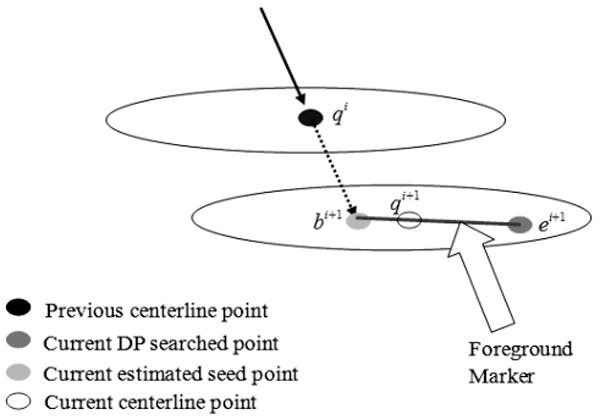
Figure 3 illustrates how seed points and DP searched points are estimated for overlapping axon objects as well as a single axon object. The dashed arrow lines represent the directional vectors that link the two centerline points on the previous two slices. The points obtained by searching from the centerline points on the previous slice along the dashed directional vectors to the current slice are used as the estimated seed points. The solid arrow lines represent the directional vectors that link the two centerline points on the previous slice and on the current slice, which could be seen as “corrected” directional vectors for the current slice. The dashed square regions represent the search regions centered at the estimated seed points. It can be seen that these search regions are large enough to cover the axon objects.

Figure 3.

Selection of marker points for (a) single axon object and (b) two attaching axon objects. The solid arrow lines represent true tracking vectors between two adjacent slices. The dashed lines represent the vectors used by the current slice to estimate marker points from the previous slice. This point, DP searched point, and the line linking them define the marker used in watershed segmentation. Notice that since the two axon objects may be very close to each other, the DP tracking may find centerline points that are very close or even the same for different axon objects. This will lead to missing axons. When marker-controlled watershed segmentation is used, different axons can be distinguished to ensure correct extraction.

We also illustrate the case of overlapping multiple axon objects. In this situation, the search regions of such axon objects will have a significant overlap. Thus, the DP search may result in a possible miss of axon objects. To address this problem, we propose marker-controlled watershed segmentation to distinguish overlapping axon objects. Thus, the DP searched points can be adjusted to the correct centerline points.

A special case is for the second slice. Since there is no linking directional vector from the previous slice, we use the directional vector that is parallel to the z-axis to estimate the seed points on the second slice. Later in this article, we show that the estimated seed points are also used as part of the markers (see section 2.3.2).

Searching for the optimal path consists of two steps. In the first step, every point in the image volume is assigned a similarity measurement to 3D line structures using the 3D line filtering method. Previous research in modeling multidimensional line structure is exemplified by the work of Steger et al. and Sato et al. (Haralick, Watson, & Laffey, 1983; Koller, Gerig, Szekely, & Dettwiler, 1995; Lorenz, Carlsen, Buzug, Fassnacht, & Weese, 1997; Sato, Araki, Hanayama, Naito, & Tamura, 1998; Sato, Nakajima et al., 1998; Steger, 1996, 1998). In this project, the 3D line filtering is achieved by using the Hessian matrix, a descriptor that is widely used to describe the second-order structures of local intensity variations around each point in the 3D space. The Hessian matrix for a pixel p at location (x, y, z) in a 3D image volume I is defined as

$${\nabla }^{2}I\left(p\right)=\left(\begin{array}{ccc}{I}_{xx}\left(p\right)& I_{xy}\left(p\right)& I_{xz}\left(p\right)\\ I_{yx}\left(p\right)& I_{yy}\left(p\right)& I_{yz}\left(p\right)\\ I_{zx}\left(p\right)& I_{zy}\left(p\right)& I_{zz}\left(p\right)\end{array}\right),$$ (2.3)

where I_xx (p) represents the partial second-order derivative of the image at point p along the x direction and I_yz (p) is the partial second-order derivatives of the image along the y and z directions, and so on. The eigenvalues of ∇²I (p) are used to define a similarity that evaluates how close a point is to a 3D line structure. Figure 4 shows the geometric relationship between three 3D objects (3D line, 3D sphere, and 3D sheet) and their eigenvalues and eigenvectors. The length and direction of the arrows in the figure represent eigenvalues and eigenvectors. Denote the three eigenvalues as λ₁, λ₂, λ₃ in descending order (that is, |λ₁| ≥ |λ₂| ≥ | λ₃|); it is clear that an ideal 3D line has the following properties:|λ₁| ≈ |λ₂| ≫ |λ₃| ≈ 0. Then the similarity measure η (p) for point p is calculated as follows:

Figure 4.

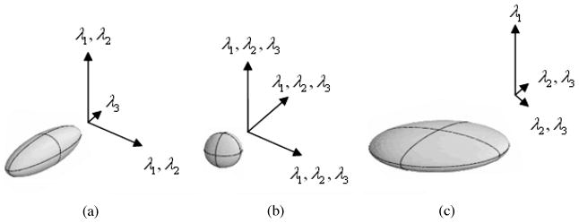
Geometric relationship between 3D objects and their eigenvalues and eigenvectors of the Hessian matrix. (a) 3D line. (b) 3D sphere. (c) 3D sheet. The length and direction of the vectors show the eigenvalues and eigenvectors for each 3D object.

$$\eta \left(p\right)=\{\begin{array}{ll}\left|{\lambda }_2\right|+{\lambda }_3,& \text{if}{\lambda }_1<0,{\lambda }_2<0,{\lambda }_3\le 0\\ \left|{\lambda }_2\right|-\frac{{\lambda }_3}{4},& \text{if}{\lambda }_1<0,{\lambda }_2<0,0<{\lambda }_3<4\left|{\lambda }_2\right|.\hfill \\ 0& \text{otherwise}\end{array}$$ (2.4)

Notice that the value of η(p) is always greater than or equal to zero. We include the second case (that is, if λ₁ < 0, λ₂ < 0, 0 < λ₃ < 4|λ₂|) due to the reason that when λ₃ > 0, the corresponding 3D line structure has concavity involved. If we use |λ₂| − λ₃ to calculate the similarity measure in this case, the true line structure could be fragmented at concave locations. Thus, we need to reduce the influence of λ₃ when λ₃ is large and positive. Experiments show that by using $|{\lambda }_2|-\frac{{\lambda }_3}{4}$ as the similarity measure, the fragmentation can be reduced to better segment 3D line structures.

By defining this measure, it is possible that the algorithm distinguishes 3D line structures from sheetlike and spherelike structures. The higher the value of η(p), the more likely it is that the point belongs to a 3D line structure. The highest value of η(p) is expected to indicate a centerline point that is located near or on the centerline, a filled tubelike structure commonly seen in our 3D axon images. We further convert η(p) to a cost value c(p) for point p as follows:

$$c\left(p\right)=1-\frac{\eta \left(p\right)}{{max}_{p\in I}\left\{\eta \left(p\right)\right\}}.$$ (2.5)

The value of c(p) decreases if the point goes near the centerline of the 3D line structure, and it is minimized on the centerline.

In the second step, we search for an optimal path for each point within the search region on the current slice to the centerline points on the previous slice. The searching method is similar to the DP technique for 2D centerline extraction, as described in Zhang et al. (2007). The difference is that the searching is applied on the 3D space, and we search for the optimal paths for multiple axons simultaneously, not one by one. Only two slices are involved in the search. Thus, the processing time is significantly reduced. The cost of linking from point p to point q in the 3D space is determined by the gradient directions of the two points. Let $\overrightarrow{d_p}$ denote the unit vector of the gradient direction at p and $\overrightarrow{n_p}$ the unit vector perpendicular to $\overrightarrow{d_p}$. Then:

$$\begin{array}{l}{\overrightarrow{d}}_p=[u_x\left(p\right),u_y\left(p\right),u_z\left(p\right)]\\ {\overrightarrow{n}}_p=\{\begin{array}{ll}[u_z\left(p\right),u_y\left(p\right),u_x\left(p\right)],& \text{if}{u}_x\left(p\right)=0\text{and}{u}_y\left(p\right)=0,\\ \left[\frac{u_x\left(p\right)u_z\left(p\right)}{u_{xy}\left(p\right)},\frac{u_y\left(p\right)u_z\left(p\right)}{u_{xy}\left(p\right)},-u_{xy}\left(p\right)\right],& \text{otherwise}\end{array}\end{array}$$ (2.6)

where u_x(p), u_y(p), u_z(p) represent the unit vectors along x, y, z directions of p, respectively. $\overrightarrow{n_p}$ is obtained by rotating $\overrightarrow{d_p}$ 90 degrees counterclockwise on the x-y plane and dividing u_z (p) into two components along the x and y directions, respectively. $u_{xy}\left(p\right)=\sqrt{u_x^2\left(p\right)+u_y^2\left(p\right)}$. The linking cost between p and q is

$$d\left(p,q\right)=\frac{2}{3\pi }\left[{cos}^{-1}\left(\overrightarrow{n_p}•\overrightarrow{v_{pq}}\right)+{cos}^{-1}\left(\overrightarrow{v_{pq}}•\overrightarrow{n_q}\right)\right],$$ (2.7)

where $\overrightarrow{v_{pq}}$ is the normalized bidirectional link between p and q:

$$\overrightarrow{v_{pq}}=\{\begin{array}{ll}\frac{\overrightarrow{q}-\overrightarrow{p}}{\Vert \overrightarrow{p}-\overrightarrow{q}\Vert };& \text{if}\overrightarrow{n_p}•(\overrightarrow{q}-\overrightarrow{p})\ge 0\\ \frac{\overrightarrow{p}-\overrightarrow{q}}{\Vert \overrightarrow{p}-\overrightarrow{q}\Vert };& \text{if}\overrightarrow{n_p}•(\overrightarrow{q}-\overrightarrow{p})<0\end{array},$$ (2.8)

where p⃗ = [p_x, p_y, p_z] and q⃗ = [q_x, q_y, q_z] are the vectors of the two points (p, q) represented by their coordinates. $\overrightarrow{v_{pq}}$ is calculated such that the difference between p⃗ and the linking direction is minimized. The linking cost between p and q, if calculated by formula 2.7, yields a high value if the two points have significantly different gradient directions or the bidirectional link between them is significantly different from either of the two gradient directions. The coefficient $\frac{2}{3\pi }$ is used to normalize the linking cost d(p, q). It is obtained from the fact that (1) the minimum possible angle between $\overrightarrow{v_{pq}}$ and $\overrightarrow{n_p}$ is 0 degree such that $\overrightarrow{n_p}•\overrightarrow{v_{pq}}\to 0$ and ${cos}^{-1}(\overrightarrow{n_p}•\overrightarrow{v_{pq}})\to \frac{\pi }{2}$, and (2) the maximum possible angle between $\overrightarrow{v_{pq}}$ and $\overrightarrow{n_q}$ is 180 degrees, such that $\overrightarrow{v_{pq}}•\overrightarrow{n_q}\to -1$ and ${cos}^{-1}(\overrightarrow{v_{pq}}•\overrightarrow{n_q})\to \pi$. Thus, the maximum possible value of ${cos}^{-1}(\overrightarrow{n_p}•\overrightarrow{v_{pq}})+{cos}^{-1}(\overrightarrow{v_{pq}}•\overrightarrow{n_q})$ is $\frac{3\pi }{2}$.

The total cost value of linking point p and q can be calculated as follows:

$$\text{Cost}\left(p,q\right)=w_c\left[c\left(p\right)+c\left(q\right)\right]+w_{d}d\left(p,q\right),$$ (2.9)

where c(p) is the local cost of p and can be calculated by formula 2.5, and d(p, q) is the linking cost from p to q and is calculated by formula 2.7. w_c, w_d are weights of local cost and linking cost, respectively. By default, w_c = 0.4, w_d = 0.2. w_c, w_d are selected based on how the two factors (local cost and linking cost) are expected to affect the DP search result. If the DP search is affected more by local cost than by linking cost, then w_c should increase and w_d should decrease, and vice versa, as long as condition 2w_c + w_d = 1 is satisfied. The DP searched point for an axon object (denoted as e^j for the jth slice) is selected as follows:

$$e^j=\underset{p\in S}{argmin}\left\{\text{Cost}\left(p,q^{j-1}\right)\right\},$$ (2.10)

where q^j−1 denotes the jth centerline point on the jth slice. That means that the point with the minimum overall cost to the previous centerline point is selected as the DP searched point.

In summary, the steps of DP-based optimal path searching are as follows:

• Step 1: Calculate the Hessian matrix for all image slices using formula 2.3.

• Step 2: Calculate the similarity measure for each point in the image volume using formula 2.4, and convert it to the cost value using formula 2.5.

• Step 3: Search for an optimal path for each point within the search region on the current slice to the centerline points on the previous slice.

• Step 4: Find the optimal path with minimal overall cost calculated by formula 2.9. The corresponding point is used as the DP searched point and will be adjusted in the following marker-controlled watershed, segmentation.

2.3.2 Marker-Controlled Watershed Segmentation

One difficult problem about 3D centerline extraction is that some 3D objects may overlap or go across others in 3D space. If two centerlines are close enough, the extraction process described may combine two centerlines as one centerline, and the other centerline will be completely missed (see figure 8 as an example). We address this problem by using the marker-controlled watershed to segment different axon objects on one slice. The centroids of segmented regions are then used to refine the locations of the centerline points.

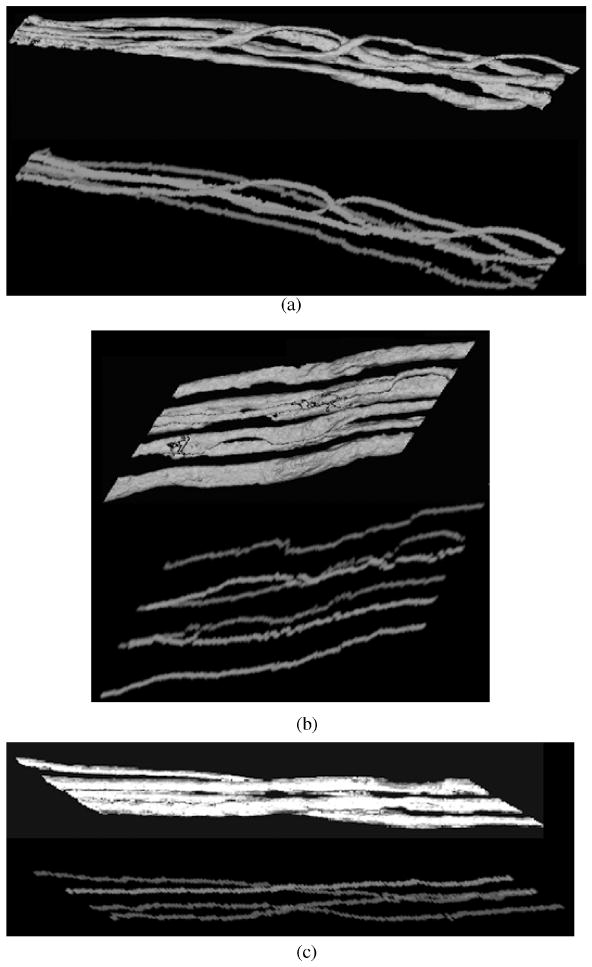
Figure 8.

Two partial 3D centerline extraction results to show the power of marker-controlled watershed segmentation. (a) Surface rendering of the original 3D axon image volume. (b) Extracted 3D centerlines without marker-controlled watershed segmentation. (c) Extracted 3D centerlines with marker-controlled watershed segmentation. Notice that the axons are overlapped at the location indicated by arrows. We observe that one axon (indicated by dotted circles) is missing in each example without marker-controlled watershed segmentation.

The watershed transform has been widely used for image segmentation (Gonzalez & Woods, 2002). It treats a gray-scale image as a topographic surface and floods this surface from its minima. If the merging of the water coming from different sources is prevented, the image is then partitioned into different sets: the catchment basins and the watershed lines that separate different catchment basins. Watershed transformation has been used as a powerful morphological segmentation method. It is usually applied to gradient images due to the reason that the contours of a gray-scale image can be viewed as the regions where the gray levels exhibit the fastest variations, that is, the regions of maximal gradient (modulus). The major reason to use watershed transformation is that it is well suited to the problem of separating overlapping objects (Beucher & Meyer, 1990; Dougherty, 1994; Yan, Zhao, Wang, Zelenetz, & Schwartz, 2006). These methods calculate from an original image its distance transform (i.e., to transform each pixel to its minimal distance to the background). If the opposite of the distance transform is regarded as the topological surface, the watershed segmentation can well separate overlapping objects from the image.

However, if the watershed transform is directly applied on gradient images, it usually results in oversegmentation: the images get partitioned in far too many regions. This is mainly due to noise and inhomogeneity in images: noise and inhomogeneity in original images result in noise and inhomogeneity in their gradient images, and this will lead to far too many regional minima (in other words, far too many catchment basins). The major solution to the problem of oversegmentation is a marker-controlled watershed, which defines new markers for the objects and floods the topographic surface from these markers. By doing this, the gradient function is modified such that the only minima are the imposed markers. Thus, the most critical part of the method is how to define markers for the objects to be extracted. In this project, for each axon object, two points can be found automatically: a seed point estimated from the previous image slice and a DP searched point from DP-based optimal path searching. These two points can be used as the object markers for watershed transform.

The marker-controlled watershed procedure in this work is as follows:

1. Calculate the gradient image from the original image slice. The magnitude of the image gradient at point p is calculated as follows:

   $$|\nabla I\left(p\right)|=\sqrt{{\left(\frac{\partial I\left(p\right)}{\partial x}\right)}^2+{\left(\frac{\partial I\left(p\right)}{\partial y}\right)}^2}.$$ (2.11)

2. Calculate foreground markers. Foreground markers consist of estimated seed points, DP searched points, and the line linking them. We involve both the estimated seed point and DP searched point as foreground markers to ensure that the watershed segmentation is correct if the DP searched point is located near the boundary of axon objects. Figure 5 shows how the foreground marker is selected.

3. Calculate background markers. First, the original image is segmented into foreground and background using a global threshold (Otsu, 1979). Second, we apply distance transform to image background. Third, we apply conventional watershed transform to the result of distance transform and keep only the watershed ridge lines as background markers.

4. Modify the gradient image so that the regional minima are at the locations of foreground and background markers.

5. Apply marker-controlled watershed transform to the modified gradient image.

6. Calculate the centroids of the segmented regions, and use the results to adjust DP searched points to centerline points if necessary.

Figure 5.

Foreground marker selection.

Let ${\text{q}}_i^j$ denote the ith centerline point on slice (j), ${\text{e}}_i^j$ denote the ith DP searched point on slice (j), and ${\text{g}}_i^j$ denote the ith centroid point on slice (j). Then ${\text{q}}_i^j$ is determined as follows:

$${\text{q}}_i^j=\{\begin{array}{ll}{\text{g}}_i^j& \text{if}\Vert {\text{g}}_i^j-{\text{q}}_i^{j-1}\Vert \le {\epsilon }_i\text{and}\Vert {\text{g}}_i^j-{\text{e}}_i^j\Vert \le {\epsilon }_i,\\ {\text{e}}_i^j& \text{otherwise}\end{array}$$ (2.12)

where $\Vert {\text{g}}_i^j-{\text{q}}_i^{j-1}\Vert$ is the 2D distance between the two points ${\text{g}}_i^j$ and ${\text{q}}_i^{j-1}$, that is, the distance between two voxels if only the x-y coordinates are considered. ε_i is the maximum centerline point deviation for the ith axon object. Equation 2.12 means that if the distance between segmented centroid point and previous centerline point or DP searched point is within the maximum possible deviation, the centroid point will then be used as the detected centerline point; otherwise, DP searched point will be used as the detected centerline point. This is important in ensuring the robustness of the algorithm in case the watershed segmentation goes wrong on a certain slice. The value of ε_i is determined as

$${\epsilon }_i=\frac{max\left\{\left|x_i^1-x_i^{\text{Z}}\right|,\left|y_i^1-y_i^{\text{Z}}\right|\right\}}{\text{Z}}$$ (2.13)

for an image volume with Z number of slices, with each slice having a size of M × N. The values of $x_i^1$, $x_i^{\text{Z}}$, $y_i^1$, $y_i^{\text{Z}}$ can be determined by manually examining the first and the last slice for each axon object in the image volume. In this work, we use ε_i = ε = max_i {ε_i} for simplicity. That is, the users need to find one centerline point on the first slice and another centerline point on the final slice so that the two points are the farthest among all possible pairs of centerline points. Note that the two points need not belong to the same axon object. The total centerline deviation is obtained by examining the coordinate difference between these two points. Then ε is calculated as the total centerline deviation divided by total number of slices.

It may be possible that the number of segmented regions is smaller than that of the axon objects after the marker-controlled watershed segmentation. This could happen when the global threshold calculated by Otsu (1979) is relatively high for some object regions with low-intensity values. Thus, the foreground marker may locate inside the background area. To address this problem, we iteratively reduce the threshold value to 90% of the previous threshold value until we obtain the same number of segmented regions as the number of axon objects, or until a predefined maximal iteration loops. If the loop reaches the predefined maximal iteration and the number of segmented regions is still fewer than that of previous slice, we use just the DP searched point for the missing region as the centerline point.

Figure 6 illustrates the above marker-controlled watershed segmentation procedure. Figure 6a is the original image slice, and Figure 6b gives the segmentation result using conventional watershed. It is obvious that the image is oversegmented. Figures 6c and 6g are the gradient images before and after the modification using markers. We observe that the regional minima are better defined by the markers in Figure 6g than those in 6c. Figure 6e shows five foreground markers. These markers are obtained by detecting five minimal cost points if connected to five centerline points in the preceding slice. Figure 6h gives the marker-controlled watershed segmentation result. The five smallest regions are considered to adjust the centerlines for the current slice.

Figure 6.

Example of marker-controlled watershed segmentation. (a) Original image slice. (b) Conventional watershed segmentation result. (c) Gradient image. (d) Distance transform of image background. (e) Foreground markers. (f) Background markers. (g) Modified gradient image. (h) Marker-controlled watershed segmentation result.

3 Results

3.1 Three-Dimensional Axon Extraction Results

We apply our 3D centerline extraction algorithm on test image volumes obtained partially from the 3D axon images as shown in Figure 1. A typical test image volume has a total of 512 slices (43 × 512 for each slice). Figure 7 shows three extraction results along with 3D views of image surface rendering. The number of axon objects in the test image volumes is 5, 6, and 4, respectively. Our method can completely extract all the centerlines for multiple axons in 3D space. The extraction is accurate when the axons are overlapping or going across each other, as shown in the figure. Figure 8 shows partial extraction results with and without marker-controlled watershed segmentation. It shows that the marker-controlled watershed helps to segment overlapping axon objects. Without watershed segmentation, DP search gives the wrong extraction at locations where multiple axons are overlapping. Figure 9 shows extraction results on 2D slices for overlapping multiple axons. The extracted centerline points are labeled by gray scales and are superimposed on the original image to show the extraction performance. Different gray scales represent different axon objects. Our method can accurately extract centerline points and distinguish different axon objects in these slices.

Figure 7.

3D centerline extraction results for (a) data#116, (b) data#242, (c) data#260. The results are shown in different gray scales. For each example, the image on the top is the 3D view of the surface rendering for the original image; the image at the bottom is the extracted centerlines.

Figure 9.

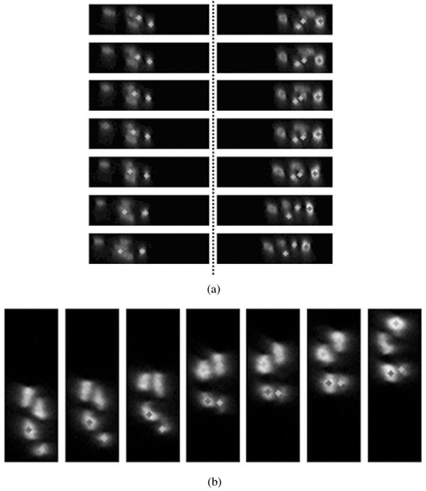
3D centerline extraction results are displayed and superimposed on the original image slices. Different gray-scale points represent centerline points for different axon objects. Notice that when the axons are attaching together, our proposed method is able to accurately separate them and correctly extract the centerline points. (a) Results for data#116. The left column shows the results from slice#97 to slice#123; the right column shows the results from slice#251 to slice#262. (b) Results for data#260. It shows the results from slice#61 to slice#83 (not all the slices in the range; only typical ones are shown).

3.2 Result Comparison

We have tested and compared our result with those of the repulsive snake model (Cai et al., 2006) and region-based active contour (RAC) method (Li, Kao, Gore, & Ding, 2007). Snakes are deformable curves that can move and change their shape to conform to object boundaries. The movement and deformation of snakes are controlled by internal forces, which are intrinsic to the geometry of the snake and independent of the image, and external forces, which are derived from the image. As an extension of the conventional snake model, the gradient vector flow (GVF) model (C. Xu & Prince, 1998) uses the vector field as the external forces such that it yields a much larger capture range than the standard snake model and is much less sensitive to the choice of initialization, to improve the detection of concave boundaries. To extend the GVF model to address the problem of 3D axon extraction, Cai et al. (2006) proposed a GVF snake model based on repulsive force among multiple objects. They exploit the prior information of the previously separated axons and employ a repulsive force to push the snakes toward their legitimate objects. The repulsive forces are obtained by reversing the gradient direction of neighboring objects. In their method, the users need to define the initial boundaries and centerline points for the first slice. They use the final contour of slice n as the initialization contour for slice (n+1), assuming that the axons do not change their positions and shapes much between consecutive slices. Their method fails at locations where the axons change shape irregularly or when the boundaries of the axons are blurred, common cases in the test axon images. Another problem of their method is that it involves several parameters that may significantly affect the extraction performance, for example, the weighting factor θ and the reliability degree d (i) used to adaptively adjust the repulsive force. Users need to iteratively adjust these parameters in order to run the snakes, and the values may not be consistent throughout the entire image slices.

The region-based active contour method (Li et al., 2007) is able to accurately segment images with noise and intensity inhomogeneity using local image information. The local image information is obtained by introducing a kernel function of local binary fitting energy and incorporating it into a variational-level set formulation. Such a variational-level set formulation does not require reinitialization, which significantly reduces running time. This method, however, requires manual settings of initial contours for all the image slices.

To compare our method with the method proposed by Cai et al. (2006) and Li et al. (2007), we carefully adjust the parameters to an optimal state for the methods and fix them for the image volume. Since the programs provided by Cai et al. and Li et al. only give boundaries of the detected objects, we assume that the centroids of the areas circled by the detected boundaries are the detected centerline points. The results by the three methods are compared in Figure 10. The test images set used are slices 53 and 106 in data set #116 and slice 10 in data set #260. It shows that the repulsive snake model cannot accurately extract axon boundaries for some slices in the image volume; thus, the detected centerline points are not accurate. The RAC contour method can accurately extract boundaries but fails to separate overlapping axon objects. Our method outperforms the repulsive snake model and RAC method in both extraction performance and the requirement of manual initialization (it requires centerline points only on the first slice).

Figure 10.

Result comparison among our proposed method, the method by Cai et al. (2006) and the method by Li et al. (2007). From top to bottom, boundary extraction results by Cai et al. and Li et al. and centerline point extraction results by our method for (a) slice 53 in dataset #116, (b) slice 10 in dataset #260, and (c) slice 106 in dataset #116. For each test result, the image on the left is obtained by Cai et al.'s method; the image in the middle is obtained by Li et al.'s method; the image on the right is obtained by our method. It is clear to see that Cai et al.'s method performs poorly in a and b. Li et al.'s method can accurately extract boundaries but fails to separate overlapping objects, as shown in a and c.

To quantitatively compare our method with the above two methods, we use the number of topological mistakes as the measure. It is defined as the number of manually labeled axons minus number of automated labeled axons. We use four full data sets to do the comparison. Table 1 shows the number of axon objects extracted and the topological mistakes for two independent manual extractions, snake-based method, RAC method, and our method. It is clear that our proposed method can extract all the axon objects seen by manual extraction.

Table 1.

Result Comparison Using Number of Axon Objects Extracted and Topological Mistakes.

Method	Manual 1	Manual 2	Snake	RACa	Ours
Data #116	5	5	3	3	5
Data #242	6	6	4	5	6
Data #260	4	4	4	4	4
Data #279	7	7	4	5	7
Total extracted	22	22	15	17	22
Topological mistakes	0	0	7	5	0

Note: The region-based active contour method.

3.3 Validation

Apart from visual inspection of the automatic results and manual results, we use the following experiment to quantitatively evaluate our proposed method for 3D axon extraction. We randomly select 10 different axon objects from the processed image volumes using our method. Two independent individuals manually select the centerline points slice by slice for those 10 axon objects. The manual labeling processes are completely independent and blind to the automated results. We then use length difference and centerline deviation to quantitatively measure the difference between automated results and manual results. The length difference (φ) is defined as follows: $\phi =|1-\frac{L_M}{L_A}|$, where L_M is the length of one axon centerline extracted manually and L_A is the length of the same axon centerline generated by the algorithm, both in 3D space. The centerline deviation (ϕ) is calculated as the number of pixels in the region surrounded by automated centerline and manually labeled centerline per automated centerline length:

$$\varphi =\frac{\text{Pix}\left(l_A,l_M\right)}{L_A},$$ (3.1)

where l_A and l_M are the automated axon centerline, and the manual axon centerline, respectively, for the same axon object. Pix(l_A, l_M) represents the number of pixels in the region surrounded by l_A and l_M. Since it is difficult to count the number of pixels between two 3D lines, we use the following method to estimate Pix(l_A, l_M): let pⁿ denote the automated centerline point on slice (n) and qⁿ the manual centerline point on the same slice. Then the two 3D centerlines from slice (n) to slice (n+1) are defined as pⁿ ↔ pⁿ⁺¹ and qⁿ ↔ qⁿ⁺¹, where a ↔ b indicates a line with two ending points a, b. The total number of pixels (pix^n,n+1) surrounded by pⁿ ↔ pⁿ⁺¹ and qⁿ ↔ qⁿ⁺¹ is estimated as the number of pixels in a 2D square, which can cover all of four points, pⁿ, pⁿ⁺¹, qⁿ, qⁿ⁺¹, if projected onto the same slice. Then we have

$$\text{Pix}\left(l_A,l_M\right)=\sum _{i=1}^{\text{Z}-1}pi{x}^{i,i+1},$$ (3.2)

where Z is the total number of slices.

Figure 11 shows the mean and standard deviation for length difference (φ) and centerline deviation (ϕ) and compares the results of the two manual extractions. We can observe that the two manual results are very similar in terms of φ and ϕ. Table 2 shows the values of mean and standard deviation for φ and ϕ. We calculate the p-values of φ and ϕ using the two-sided paired t-test and list the result in Table 2. The p-values are all greater than 0.05, which quantitatively proves that the two manual results are similar. Table 3 lists the Pearson linear correlation coefficients of φ and ϕ, which shows that there exists a strong correlation in the automated results and the manual results. We calculate the cumulative distribution of φ and ϕ, respectively, using Kolmogorov-Smirnov goodness-of-fit hypothesis test (Nimchinsky, Sabatini, & Svoboda, 2002) and compare the quantile-quantile plots of the two manual results in Figure 12. It shows a linear-like quantile-quantile plots and similar cumulative distribution functions for the three sets of results.

Figure 11.

Box plots for the length difference and centerline deviation between two manual extractions. The middle line is the mean value for each data set. The upper line of the box is the upper quartile value. The lower line of the box is the lower quartile value. (a) Length difference comparison between two manual results. (b) Centerline deviation comparison between two manual results.

Table 2.

Mean and Standard Deviation Values for the Two Manual Results.

	φ			ϕ
	Mean	SD	p-value	Mean	SD	p-value
Result 1	0.0515	0.0861	0.3352	2.3381	0.4293	0.6661
Result 2	0.0622	0.0654		2.1758	0.3686

Table 3.

Pearson Linear Correlation Coefficients Among the Automated Result, the Manual Result 1, and Manual Result 2.

	φ			ϕ
	Auto	Result 1	Result 2	Auto	Result 1	Result 2
Auto result	-	0.9873	0.9907	-	-	-
Result 1	0.9873	-	0.9993	-	-	0.9660
Result 1	0.9907	0.9993	-	-	0.9660	-

Figure 12.

Quantile-quantile plots of the length of the axon centerlines for (a) automated versus manual result 1. (b) Automated versus manual result 2. Quantile-quantile plots of the centerline deviation for (c) manual result 1 versus manual result 2. Cumulative distributions of the length of the axon centerlines for (d) automated (circle markers) versus manual result 1 (star markers); (e) automated (circle markers) versus manual result 2 (star markers). Cumulative distributions of the centerline deviation for (f) manual result 1 (circle markers) versus manual result 2 (star markers).

4 Conclusion

We presented a novel algorithm for extracting the centerlines of the axons in the 3D space. The algorithm is able to automatically and accurately track multiple 3D axons in the image volume using 3D curvilinear structure detection. Our proposed method is able to extract centerline and boundaries of 3D neurite structures in 3D microscopy axon images. The extraction is highly automated, rapid, and accurate, making it suitable for replacing the fully manual methods of extracting curvilinear structures when studying 3D axon images. The proposed method can handle complicated axon structures such as cross-over sections and overlapping objects.

Future work will focus on extracting more complicated axon structures in the 3D space. An example of more complicated cases is shown in Figure 13. Some axon structures go through the same slice twice and may change directions sharply. We will study a sophisticated model for extracting such axon structures.

Figure 13.

An example 3D axon image volume with very complicated axon structures. In this case, one axon may go across the same slice twice and may change directions very sharply.

References

- Adams R. Radial decomposition of discs and spheres. Computer Vision, Graphics, and Image Processing: Graphical Models and Image Processing. 1993;55(5):325–332. [Google Scholar]
- Al-Kofahi KA, Lasek S, Szarowski DH, Pace CJ, Nagy G, Turner JN, et al. Rapid automated three-dimensional tracing of neurons from confocal image stacks. IEEE Transactions on Information Technology in Biomedicine. 2002;6(2):171–187. doi: 10.1109/titb.2002.1006304. [DOI] [PubMed] [Google Scholar]
- Amini AA, Weymouth TE, Jain RC. Using dynamic programming for solving variational problems in vision. IEEE Transactions Pattern Analysis and Machine Intelligence. 1990;12:855–867. [Google Scholar]
- Andreas H, Gerald K, Bernd M, Werner Z. Tracking on tree-like structures in 3-D confocal images. In: Carol JC, Jose-Angel C, Jeremy ML, Thomas TL, Tony W, editors. Proceedings of the Three-Dimensional and Multidimensional Microscopy: Image Acquisition and Processing V; Bellingham, WA: SPIE; 1998. [Google Scholar]
- Bellman RE, Dreyfus SE. Applied dynamic programming. Princeton, NJ: Princeton University Press; 1962. [Google Scholar]
- Beucher S, Meyer F. Morphological segmentation. Journal of Visual Communication and Image Representation. 1990;1(1):21–46. [Google Scholar]
- Bitplane. Imaris Software. 2006 Available online at http://www.bitplane.com/products/index.shtml.
- Cai H, Xu X, Lu J, Lichtman J, Yung SP, Wong STC. Repulsive force based snake model to segment and track neuronal axons in 3D microscopy image stacks. NeuroImage. 2006;32:1608–1620. doi: 10.1016/j.neuroimage.2006.05.036. [DOI] [PubMed] [Google Scholar]
- Can A, Shen H, Turner JN, Tanenbaum HL, Roysam B. Rapid automated tracing and feature extraction from live high-resolution retinal fundus images using direct exploratory algorithms. IEEE Transactions on Information Technology in Biomedicine. 1999;3(2):125–138. doi: 10.1109/4233.767088. [DOI] [PubMed] [Google Scholar]
- Capowski JJ. Computer techniques in neuroanatomy. New York: Plenum Press; 1989. [Google Scholar]
- Cohen AR, Roysam B, Turner JN. Automated tracing and volume measurements of neurons from 3-D confocal fluorescence microscopy data. Journal of Microscopy. 1994;173:103–114. doi: 10.1111/j.1365-2818.1994.tb03433.x. [DOI] [PubMed] [Google Scholar]
- Coleman PD, Garvey CF, Young J, Simon W. Semiautomatic tracing of neuronal processes. New York: Plenum Press; 1977. [Google Scholar]
- Dougherty ER. Digital image processing methods. Boca Raton, FL: CRC; 1994. [Google Scholar]
- Fiala JC. Reconstruct software. 2006 Available online at http://synapses.bu.edu/tools/index.htm.
- Garvey CF, Young J, Simon W, Coleman PD. Automated three-dimensional dendrite tracking system. Electroencephalogr Clin Neurophysiol. 1973;35:199–204. doi: 10.1016/0013-4694(73)90177-6. [DOI] [PubMed] [Google Scholar]
- Geiger D, Gupta A, Costa LA, Vlontzos J. Dynamic programming for detecting, tracking, and matching deformable contours. IEEE Transactions on Pattern Analysis and Machine Intelligence. 1995;17(3):294–302. [Google Scholar]
- Gonzalez RC, Woods RE. Digital image processing. Upper Saddle River, NJ: Prentice Hall; 2002. [Google Scholar]
- Haralick RM, Watson LT, Laffey TJ. The topographic primal sketch. International Journal of Robotics Research. 1983;2:50–72. [Google Scholar]
- He W, Hamilton TA, Cohen AR, Holmes TJ, Pace C, Szarowski DH, et al. Automated three-dimensional tracing of neurons in confocal and brightfield images. Microscopy and Microanalysis. 2003;9:296–310. doi: 10.1017/S143192760303040X. [DOI] [PubMed] [Google Scholar]
- Kasthuri H, Lichtman JW. The role of neuronal identity in synaptic competition. Nature. 2003;424:426–430. doi: 10.1038/nature01836. [DOI] [PubMed] [Google Scholar]
- Keller-Peck CR, Walsh MK, Gan WB, Feng G, Sanes JR, Lichtman JW. Asynchronous synapse elimination in neonatal motor units: Studies using GFP transgenic mice. Neuron. 2001;31:381–394. doi: 10.1016/s0896-6273(01)00383-x. [DOI] [PubMed] [Google Scholar]
- Koller TM, Gerig G, Szekely G, Dettwiler D. Multiscale detection of curvilinear structures in 2-D and 3-D image data. Proceedings of the Fifth International Conference on Computer Vision; Washington, DC: IEE Computer Society; 1995. [Google Scholar]
- Li C, Kao CY, Gore JC, Ding Z. Implicit active contours driven by local binary fitting energy. Proceedings of the IEEE Computer Society Conference on Computer Vision and Pattern Recognition; Washington, DC: IEEE Computer Society; 2007. [Google Scholar]
- Lin G, Bjornsson CS, Smith KL, Abdul-Karim AM, Turner JN, Shain W, et al. Automated image analysis methods for 3-D quantification of the neurovascular unit from multichannel confocal microscope images. Cytometry Part A. 2005;66A(1):9–23. doi: 10.1002/cyto.a.20149. [DOI] [PubMed] [Google Scholar]
- Lorenz C, Carlsen IC, Buzug TM, Fassnacht C, Weese J. Multi-scale line segmentation with automatic estimation of width, contrast and tangential direction in 2D and 3D medical images. Proceedings of the First Joint Conference on Computer Vision, Virtual Reality and Robotics in Medicine and Medial Robotics and Computer-Assisted Surgery; Berlin: Springer-Verlag; 1997. [Google Scholar]
- Meijering E, Jacob M, Sarria JCF, Steiner P, Hirling H, Unser M. Design and validation of a tool for neurite tracing and analysis in fluorescence microscopy images. Cytometry. 2004;58A(2):167–176. doi: 10.1002/cyto.a.20022. [DOI] [PubMed] [Google Scholar]
- Meyer F. Iterative image transformations for an automatic screening of cervical cancer. Journal of Histochemistry and Cytochemistry. 1979;27:128–135. doi: 10.1177/27.1.438499. [DOI] [PubMed] [Google Scholar]
- Mortensen E, Morse B, Barrett W, Udupa J. Adaptive boundary detection using “live-wire” two-dimensional dynamic programming. Paper presented at Computers in Cardiology; Durham, NC. 1992. [Google Scholar]
- Nimchinsky EA, Sabatini BL, Svoboda K. Structure and function of dendritic spines. Annual Review of Physiology. 2002;64:313–353. doi: 10.1146/annurev.physiol.64.081501.160008. [DOI] [PubMed] [Google Scholar]
- Otsu N. A threshold selection method from gray-level histograms. IEEE Transactions on Systems, Man, and Cybernetics. 1979;9(1):62–66. [Google Scholar]
- Sato Y, Araki T, Hanayama M, Naito H, Tamura S. A viewpoint determination system for stenosis diagnosis and quantification in coronary angiographic image acquisition. IEEE Transactions on Medical Imaging. 1998;17:121–137. doi: 10.1109/42.668703. [DOI] [PubMed] [Google Scholar]
- Sato Y, Nakajima S, Shiraga N, Atsumi H, Yoshida S, Koller T, et al. Three-dimensional multi-scale line filter for segmentation and visualization of curvilinear structures in medical images. Medical Image Analysis. 1998;2:143–168. doi: 10.1016/s1361-8415(98)80009-1. [DOI] [PubMed] [Google Scholar]
- Shen H, Roysam B, Stewart CV, Turner JN, Tanenbaum HL. Optimal scheduling of tracing computations for real-time vascular landmark extraction from retinal fundus images. IEEE Transactions on Information Technology in Biomedicine. 2001;5:77–91. doi: 10.1109/4233.908405. [DOI] [PubMed] [Google Scholar]
- Steger C. Extracting curvilinear structures: A differential geometric approach. Paper presented at the Fourth European Conference on Computer Vision; Cambridge, UK. 1996. [Google Scholar]
- Steger C. An unbiased detector of curvilinear structure. IEEE Transactions on Pattern Analysis and Machine Intelligence. 1998;20(2):113–125. [Google Scholar]
- Xu C, Prince JL. Snakes, shapes, and gradient vector flow. IEEE Transactions on Image Processing. 1998;7:359–369. doi: 10.1109/83.661186. [DOI] [PubMed] [Google Scholar]
- Xu F, Lewis PH, Chad JE, Wheal HV. Extracting generalized cylinder models of dendritic trees from 3D image stacks. In: Cogswell CJ, Concello JA, Lerner JM, Lu TT, Wilson T, editors. Proceedings of SPIE: Three-Dimensional and Multidimensional Microscopy: Image Acquisition and Processing V; Bellingham, WA: SPIE; 1998. [Google Scholar]
- Yan J, Zhao B, Wang L, Zelenetz A, Schwartz LH. Marker-controlled watershed for lymphoma segmentation in sequential CT images. Medical Physics. 2006;33(7):2452–2460. doi: 10.1118/1.2207133. [DOI] [PubMed] [Google Scholar]
- Zhang Y, Zhou X, Degterev A, Lipinski M, Adjeroh D, Yuan J, et al. Automated neurite extraction using dynamic programming for high-throughput screening of neuron-based assays. NeuroImage. 2007;35(4):1502–1515. doi: 10.1016/j.neuroimage.2007.01.014. [DOI] [PMC free article] [PubMed] [Google Scholar]