

Abstract
Recent studies have shown that most neurons in the dorsal medial superior temporal area (MSTd) signal the direction of self-translation (i.e., heading) in response to both optic flow and inertial motion. Much less is currently known about the response properties of MSTd neurons during self-rotation. We have characterized the three-dimensional tuning of MSTd neurons while monkeys passively fixated a central, head-fixed target. Rotational stimuli were either presented using a motion platform or simulated visually using optic flow. Nearly all MSTd cells were significantly tuned for the direction of rotation in the absence of optic flow, with more neurons preferring roll than pitch or yaw rotations. The preferred rotation axis in response to optic flow was generally the opposite of that during physical rotation. This result differs sharply from our findings for translational motion, where approximately half of MSTd neurons have congruent visual and vestibular preferences. By testing a subset of neurons with combined visual and vestibular stimulation, we also show that the contributions of visual and vestibular cues to MSTd responses depend on the relative reliabilities of the two stimulus modalities. Previous studies of MSTd responses to motion in darkness have assumed a vestibular origin for the activity observed. We have directly verified this assumption by recording from MSTd neurons after bilateral labyrinthectomy. Selectivity for physical rotation and translation stimuli was eliminated after labyrinthectomy, whereas selectivity to optic flow was unaffected. Overall, the lack of MSTd neurons with congruent rotation tuning for visual and vestibular stimuli suggests that MSTd does not integrate these signals to produce a robust perception of self-rotation. Vestibular rotation signals in MSTd may instead be used to compensate for the confounding effects of rotatory head movements on optic flow.
Keywords: monkey, MST, optic flow, vestibular, visual motion, rotation
Introduction
Perception of spatial orientation and self-motion can benefit from integration of multiple sensory cues, including visual, vestibular, and somatosensory signals (Telford et al., 1995; Ohmi, 1996; Harris et al., 2000; Bertin and Berthoz, 2004), but the neural substrates for this sensory integration remain unclear. Patterns of optic flow across the retina have long been thought to be important for computing self-motion (Warren and Hannon, 1990; Warren, 2003). Neurons in the dorsal medial superior temporal area (MSTd) respond selectively to complex, large-field visual motion stimuli that simulate self-motion (Warren, 2003; Heuer and Britten, 2004; Logan and Duffy, 2006). Visually responsive MSTd cells have traditionally been described as selective for the planar (horizontal/vertical), radial (expansion/contraction), and circular (clockwise/counterclockwise) components of optic flow (Saito et al., 1986; Tanaka et al., 1986; Tanaka and Saito, 1989; Lagae et al., 1994; Geesaman and Andersen, 1996), or as encoding combinations of these components (e.g., spiral motion) (Tanaka et al., 1989; Duffy and Wurtz, 1991, 1997; Orban et al., 1992; Graziano et al., 1994).
If MSTd neurons do indeed combine optic flow signals with nonvisual (i.e., vestibular) information to signal self-motion, it may be more natural to describe MSTd responses in terms of three-dimensional (3D) translation and rotation components of observer motion. Using this framework, MSTd neurons were shown to represent the direction of self-translation (heading) in 3D space when presented with large-field optic flow stimuli. In addition, previous studies have shown that up to two-thirds of optic flow-sensitive MSTd neurons also code the 3D direction of translation of the head/body in the absence of optic flow (Duffy, 1998; Bremmer et al., 1999; Gu et al., 2006b). Notably, 3D heading preferences in response to inertial motion were either the same as or the opposite of heading preferences defined by optic flow [“congruent” and “opposite” cells, respectively (Gu et al., 2006b)]. Neurons with congruent visual/vestibular heading preferences may allow improved heading discrimination when cues are combined (Gu et al., 2006a).
Considerably less is currently known about MSTd responses to physical rotations. Shenoy et al. (1999) reported that 20% of optic flow-sensitive MSTd neurons showed selectivity for yaw or pitch rotation while fixating a head-fixed target. However, Ono and Mustari (2006) reported no modulation of pursuit-sensitive MSTd neurons during yaw rotation in darkness. Previous studies of posterior parietal cortex had reported modulation during whole-body rotation in areas 7a/MST (Kawano et al., 1980, 1984; Sakata et al., 1994) and in the lateral region of MST (Thier and Erickson, 1992a,b).
Notably, a comprehensive characterization of 3D visual and vestibular rotation selectivity in MSTd is still lacking. Furthermore, although MSTd responses to rotation in the absence of optic flow are often assumed to be vestibular in origin (but see, Ono and Mustari, 2006), this hypothesis has not been tested explicitly. Alternatively, tuning of MSTd neurons to inertial motion stimuli could arise, at least in part, from somatosensory signals. In this study, we characterize both the 3D rotational and 3D translational selectivity of MSTd neurons using stimuli defined by either visual (optic flow) or nonvisual (physical movement) cues. We find a conspicuous absence of MSTd neurons with congruent rotational preferences for optic flow and physical motion; instead, visual and nonvisual direction preferences are usually oppositely directed. This result, which contrasts with the relationships found for translational motion (Gu et al., 2006b), suggests different roles of MSTd in processing self-rotation versus self-translation signals. Finally, using bilateral labyrinthectomy, we show directly that nonvisual MSTd responses to rotation and translation have a vestibular origin.
Materials and Methods
Experiments were performed with four male rhesus monkeys (Macaca mulatta) weighing 5–6 kg. Because most of the general procedures were the same as those used in a previous study (Gu et al., 2006b), they will only be described here briefly. Animals were chronically implanted with a circular, molded, lightweight plastic ring (5 cm in diameter) that was anchored to the skull using titanium inverted T-bolts and dental acrylic. Monkeys were also implanted with scleral coils for measuring eye movements in a magnetic field (Robinson, 1963). All animal surgeries and experimental procedures were approved by the Institutional Animal Care and Use Committee at Washington University and were in accordance with National Institutes of Health guidelines. After sufficient recovery, animals were trained using standard operant conditioning to fixate targets for fluid reward.
Vestibular and visual stimuli.
Three-dimensional movement was delivered using a 6 df motion platform (MOOG 6DOF2000E; Moog, East Aurora, NY). The motion trajectory was controlled in real time at 60 Hz over an Ethernet interface. A three-chip digital light projector (Mirage 2000; Christie Digital Systems, Cypress, CA) was mounted on top of the motion platform to rear-project images onto a 60 × 60 cm tangent screen that was viewed by the monkey from a distance of 30 cm (thus subtending 90 × 90° of visual angle). The screen was mounted at the front of the field coil frame, with the sides, top, and bottom of the coil frame covered with opaque material, such that the monkey only saw visual patterns presented on the screen. Visual stimuli in these experiments depicted movement of the observer through a 3D cloud of “stars” that occupied a virtual space 100 cm wide, 100 cm tall, and 40 cm deep. Star density was 0.01/cm3, with each star being a 0.15 × 0.15 cm triangle. Approximately 1500 stars were visible at any time within the field of view of the screen. The display screen was located in the center of the star field before stimulus onset, and it remained well within the depth of the star field throughout the motion trajectory (for additional details, see Gu et al., 2006b).
Monkeys sat comfortably in a primate chair mounted on top of the motion platform and viewed the screen binocularly. Stereoscopic images were displayed as red/green anaglyphs and were viewed through Kodak (Rochester, NY) wratten filters (#29, #61) that were mounted in custom-made goggles. Accurate rendering of the visual motion, binocular disparity, and texture cues that accompany self-motion was achieved by moving two OpenGL cameras (one for each eye, separated by the interpupillary distance) through this space along the exact trajectories followed by the monkey's eyes. These visual stimuli contained a full set of naturalistic visual cues, except for the image blur that normally arises because of accommodation.
Electrophysiological recordings.
We recorded extracellularly the activities of single neurons from five hemispheres in four monkeys. For this purpose, an acrylic recording grid was stereotaxically fitted inside the head stabilization ring (Dickman and Angelaki, 2002). The grid extended from the midline to the area overlying MSTd bilaterally. A tungsten microelectrode (tip diameter, 3 μm; impedance, 1–2 MΩ at 1 kHz; Frederick Haer Company, Bowdoinham, ME) was advanced into the cortex through a transdural guide tube, using a micromanipulator (Frederick Haer Company) mounted on top of the monkey's head implant. Single neurons were isolated using a conventional amplifier, a bandpass eight-pole filter (400–5000 Hz), and a dual voltage–time window discriminator (BAK Electronics, Mount Airy, MD). The times of occurrence of action potentials and all behavioral events were recorded with 1 ms resolution by the data acquisition computer. Eye movement traces were low-pass filtered and sampled at 250 Hz. Raw neural signals were also digitized at 25 kHz and stored to disk for off-line spike sorting and additional analyses.
Area MSTd was first identified using magnetic resonance imaging (MRI) scans. An initial scan was performed on each monkey before any surgery using a high-resolution sagittal magnetization-prepared rapid-acquisition gradient echo sequence (0.75 × 0.75 × 0.75 mm voxels). Area MSTd was identified as a region centered ∼15 mm lateral to the midline and 3–6 mm posterior to the interaural plane. Several other criteria were applied to identify MSTd neurons during recording experiments (for details, see Gu et al., 2006b). First, the patterns of gray and white matter transitions along electrode penetrations were identified and compared with the MRI scans. Second, we mapped the receptive fields of MSTd neurons manually by moving a patch of drifting random dots around the visual field and observing a qualitative map of instantaneous firing rates on a custom graphical interface. Finally, our penetrations in the medial and posterior portions of MST were also guided by the eccentricity of receptive fields in the underlying middle temporal area (MT) (Gu et al., 2006b).
In two of the animals (Q and Z), we verified our recording locations histologically after termination of all experiments. The animals were sedated with ketamine HCl (10 mg/kg, i.m.) and deeply anesthetized with sodium pentobarbital (70 mg/kg, i.v.). They were then perfused trancardially with a buffered saline rinse [0.1 m, pH 7.2 phosphate buffer (PB)], followed by a fixative solution consisting of 4.0% paraformaldehyde in PB. Their brains were blocked in the frontal plane before removal and placed in cold fixative for 24 h. They then were cryoprotected in 30% sucrose in PB, before being frozen and sectioned on a sliding microtome. Serial 50 μm sections were collected, and every third section was mounted and counterstained with cresyl violet. The sections were then dehydrated, cleared, and coverslipped. Areas of cortex containing electrode tracks were drawn using a binocular stereoscope equipped with a drawing tube and were photographed using a photomicroscope (Eclipse 600; Nikon, Tokyo, Japan) and a digital camera (CoolSnap ES; Photometrics, Tucson, AZ). The digitized images were imported using MetaMorph software and adjusted to emulate the visualized image using Photoshop software. Examples of the electrode tracks are illustrated in Figure 1.
Figure 1.

Schematic illustration and photographs of recording sites as shown in coronal sections. A, B, Right hemisphere of monkey Z. C, D, Left hemisphere of monkey Q. Thick rectangles in the schematic illustrations show the area of magnification in the corresponding photographs. Thin vertical lines in A and C indicate examples of electrode tracks, which can also be recognized in the photos (B, D, asterisks). Dashed lines in photos indicate gray matter/white matter boundaries and the border between MST and MT. The location of these borders is based on MRI data as analyzed by CARET software (Van Essen et al., 2001).
Experimental protocol.
MSTd neurons were tested with either one or both of two sets of stimuli. The “translation protocol” consisted of straight translational movements along 26 directions corresponding to all combinations of azimuth and elevation angles in increments of 45° (Fig. 2A). This included all combinations of movement vectors having eight different azimuth angles (0, 45, 90, 135, 180, 225, 270, and 315°), each of which was presented at three different elevation angles: 0° [the horizontal plane (Fig. 2B)] and ±45° (for a sum of 8 × 3 = 24 directions). Two additional directions are specified by elevation angles of −90 and 90° (corresponding to upward and downward movement directions, respectively) (Fig. 2C). Each movement trajectory (either real or visually simulated) had a duration of 2 s and consisted of a Gaussian velocity profile (Fig. 3). Translation amplitude was 13 cm (total displacement), with a peak acceleration of ∼0.1 G (0.98 m/s2) and a peak velocity of 30 cm/s. This translation protocol was the same as that used in a previous study (Gu et al., 2006b).
Figure 2.

Schematic of the 26 rotational and translational directions used to test MSTd neurons. A, Illustration of the 26 movement vectors, spaced 45° apart, in both azimuth and elevation. B, Top view: definition of azimuth. C, Side view: definition of elevation. Straight arrows illustrate the direction of movement in the translation protocol. Curved arrows illustrate the direction of rotation (according to the right-hand rule) about each of the movement vectors.
Figure 3.
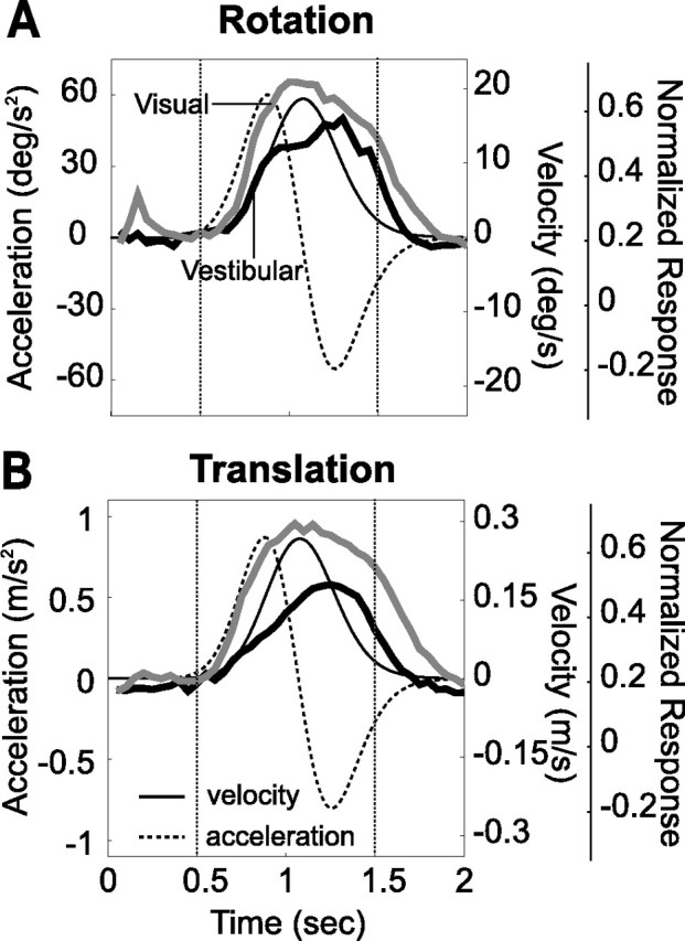
Normalized population responses to visual and vestibular stimuli (thick gray and black curves) during rotation (A) and translation (B) are superimposed on the stimulus velocity and acceleration profiles (solid and dashed black lines). The dotted vertical lines illustrate the 1 s analysis interval used to calculate mean firing rates. Data are along the preferred direction of the cell and were normalized relative to the peak visual response.
The “rotation protocol” consisted of rotations about the same 26 directions, which now represent the corresponding axis of rotation according to the right-hand rule (Fig. 2B, C). For example, azimuths of 0 and 180° (elevation, 0°) correspond to pitch-up and pitch-down rotations, respectively. Azimuths of 90 and 270° (elevation, 0°) correspond to roll rotations (right ear down and left ear down, respectively). Finally, elevation angles of −90 and 90° correspond to leftward or rightward yaw rotation, respectively. Rotation amplitude was 9°, and peak angular velocity was ∼20°/s. Note that the rotation stimuli were generated such that all axes passed through a common point that was located in the mid-sagittal plane along the interaural axis. The animal was always rotated around this point at the center of the head.
The rotation and translation protocols both included two stimulus conditions. (1) In the “vestibular” condition, the monkey was moved in the absence of optic flow. The screen was blank, except for a fixation point that remained at a fixed head-centered location throughout the motion trajectory (i.e., the fixation point moved with the animal's head). Because the apparatus was enclosed on all sides with black, opaque material, there was no change in the visual image during movement (excluding that produced by microsaccades and small fixational drifts). (2) In the “visual” condition, the motion platform was stationary, whereas optic flow simulating movement through the cloud of stars was presented on the screen. Note that all stimulus directions are referenced to body motion (real or simulated) when the data are plotted (see Fig. 4). Thus, a neuron with similar preferred directions in the visual and vestibular conditions is considered congruent.
Figure 4.

Examples of 3D direction tuning for an MSTd neuron tested during vestibular rotation (A), visual rotation (B), vestibular translation (C), and visual translation (D). Color contour maps show the mean firing rate as a function of azimuth and elevation angles. Each contour map shows the Lambert cylindrical equal-area projection of the original spherical data (see Materials and Methods). In this projection, the ordinate is a sinusoidally transformed version of elevation angle. The tuning curves along the margins of each color map illustrate mean ± SEM firing rates plotted as a function of either elevation or azimuth (averaged across azimuth or elevation, respectively).
For both the visual and vestibular conditions, the animal was required to fixate a central target (0.2° in diameter) for 200 ms before the onset of the motion stimulus (fixation windows spanned 1.5 × 1.5° of visual angle). The animals were rewarded at the end of each trial for maintaining fixation throughout the stimulus presentation. If fixation was broken at any time during the stimulus, the trial was aborted and the data were discarded.
The translation and rotationprotocols were delivered in separate blocks of trials. Within each block, visual and vestibular stimuli were randomly interleaved, along with a (null) condition in which the motion platform remained stationary and no star field was shown (to assess spontaneous activity). To complete five repetitions of all 26 directions for each of the visual/vestibular conditions, plus five repetitions of the null condition, the monkey was required to successfully complete 26 × 2 × 5 + 5 = 265 trials for each of the translation and rotation protocols. Neurons were included in the sample if each stimulus in a block was successfully repeated at least three times. For 97% of neurons, we completed all five repetitions of each stimulus.
For a subpopulation of 23 neurons in one of the animals (monkey L), we also tested cells with a “combined” condition, in which the animal was rotated by the motion platform in the presence of a congruent optic flow stimulus. The visual motion stimulus was presented at 100% coherence in this block of trials (which included interleaved visual and vestibular conditions). If single-unit isolation was maintained, the combined rotation stimulus was also delivered at a reduced visual coherence (35%) in a separate block of trials (without interleaved visual and vestibular conditions). Motion coherence was manipulated by randomly relocating a percentage of the dots within the 3D virtual volume on every subsequent frame (e.g., for 35% coherence, 65% of the dots were relocated randomly every frame).
Whenever satisfactory neuronal isolation was maintained after completion of all fixation protocols, neural responses were also collected during rotational platform motion in complete darkness (with the projector turned off). Stimuli were identical to those in the vestibular fixation protocol in terms of both rotation directions and temporal response profile. In these trials, there was no behavioral requirement to fixate, and rewards were delivered manually to keep the animal alert.
Data analysis.
Analyses and statistical tests were performed in Matlab (Mathworks, Natick, MA) using custom scripts. Normalized population responses to visual and vestibular stimuli showed that MSTd neurons roughly followed stimulus velocity (Fig. 3). Thus, for each stimulus direction and motion type, we computed the firing rate during the middle 1 s interval of each trial and averaged across stimulus repetitions to compute the mean firing rate (Gu et al., 2006b). Mean responses were then plotted as a function of azimuth and elevation to create 3D tuning functions. To plot these spherical data on Cartesian axes (see Figs. 4, 8, 11), the data were transformed using the Lambert cylindrical equal-area projection (Snyder, 1987). This produces flattened representations in which the abscissa represents azimuth angle and the ordinate corresponds to a sinusoidally transformed version of the elevation angle. Statistical significance of the response tuning of each neuron was assessed using one-way ANOVA.
Figure 8.

A–C, Examples of 3D rotation tuning for an MSTd neuron tested during both fixation and in darkness, illustrating vestibular rotation (A; fixation of a head-stationary target), visual rotation (B; fixation of a head-stationary target), and vestibular rotation in complete darkness (C). The format is as in Figure 4. D, Comparison of peristimulus time histograms from a single motion direction (azimuth, 0°; elevation, 0°) between the standard vestibular rotation condition (left) and rotation in darkness (right). Red curves indicate the time course of the motion stimulus.
Figure 11.

Examples of 3D rotation tuning for four MSTd neurons (A–D) tested during vestibular, visual, combined (100% visual coherence), and combined (35% visual coherence) conditions. The format is as in Figure 4.
To quantify spatial tuning strength, we computed a direction discrimination index (DDI), which characterizes the ability of a neuron to discriminate changes in the stimulus relative to its intrinsic level of variability (Prince et al., 2002; DeAngelis and Uka, 2003):
 |
where Rmax and Rmin are the mean firing rates of the neuron along the directions that elicited maximal and minimal responses, respectively; SSE is the sum-squared error around the mean responses; N is the total number of observations (trials); and M is the number of stimulus directions (M = 26). This index quantifies the amount of response modulation (attributable to changes in stimulus direction) relative to the noise level.
The preferred direction of a neuron for each stimulus condition was described by the azimuth and elevation of the vector sum of the individual responses (after subtracting spontaneous activity). In such a representation, the mean firing rate in each trial was considered to represent the magnitude of a 3D vector, the direction of which was defined by the azimuth and elevation angles of the particular stimulus (Gu et al., 2006b). To plot the difference in 3D preferred directions (|Δ preferred direction|) between two conditions on Cartesian axes (see Figs. 5A,B, 7C,D, 9A, 12A,B,E,F), the data were transformed using the Lambert cylindrical equal-area projection (Snyder, 1987).
Figure 5.

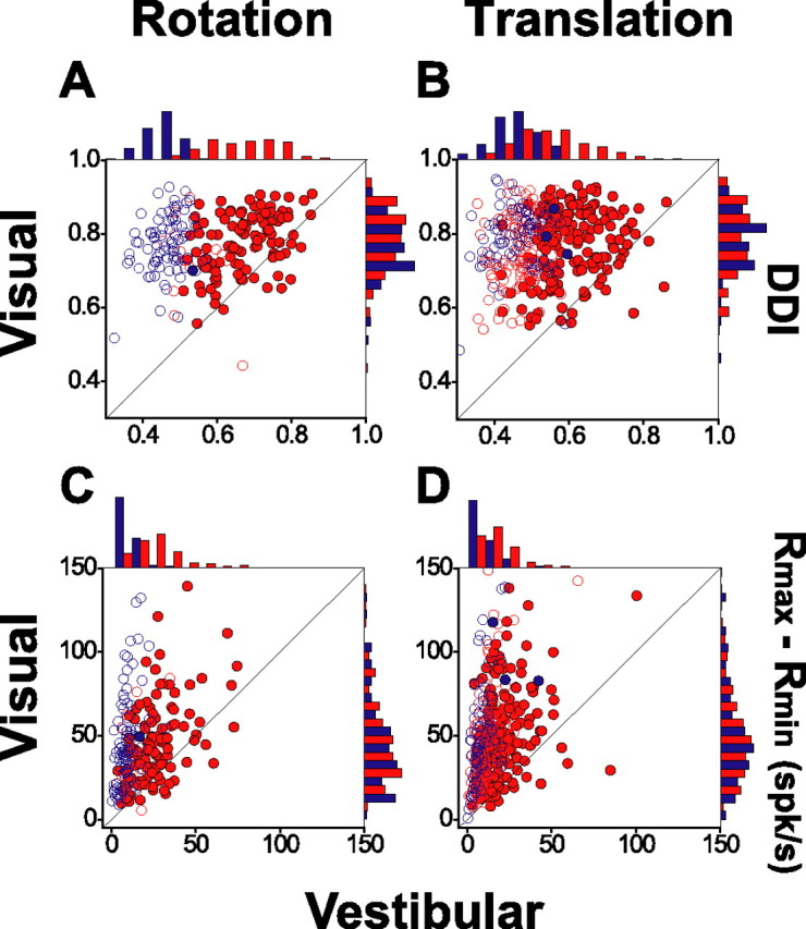
Summary of the differences in direction preference of MSTd neurons between the visual and vestibular conditions, plotted separately for rotation (left column; n = 113) and translation (right column; n = 167). A, B, Histograms of the absolute differences in 3D preferred directions between the visual and vestibular conditions (|Δ preferred direction|) for the rotation and translation protocols, respectively. Data are included only for neurons with significant 3D tuning in both stimulus conditions. C, D, Distributions of the differences in direction preference as projected onto each of the three cardinal planes: X–Z (front view), Y–Z (side view), and X–Y (top view). Note that the data from the 2D projections now cover a range of 360°.
Figure 7.
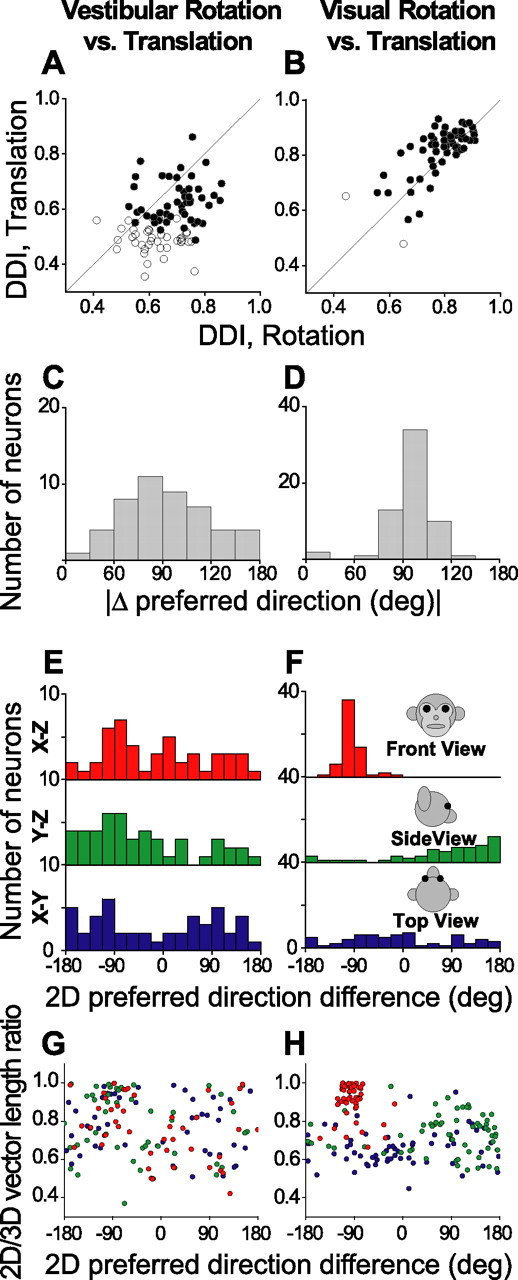
Summary of tuning strength and the differences in direction preference between rotation and translation, plotted separately for the vestibular (left column; n = 48) and visual (right column; n = 61) conditions. A, B, Scatter plots of the DDI during rotation and translation. Filled symbols indicate cells with significant tuning under both rotation and translation protocols (ANOVA, p < 0.05); open symbols denote cells without significant tuning under either one or both of the rotation and translation protocols (ANOVA, p > 0.05). C, D, Histograms of the absolute differences in 3D preferred direction (|Δ preferred direction|) between rotation and translation for the vestibular and visual conditions, respectively (calculated only for neurons with significant tuning in both conditions). E, F, Distributions of preferred direction differences as projected onto each of the three cardinal planes: X–Z (front view), Y–Z (side view), and X–Y plane (top view). G, H, The ratio of the lengths of the 2D and 3D preferred direction vectors is plotted as a function of the corresponding 2D projection of the difference in preferred direction (red, green, and blue circles for each of the X–Z, Y–Z, and X–Y planes, respectively).
Figure 9.
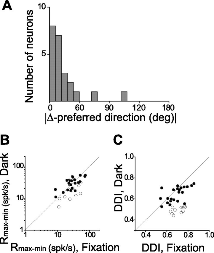
Population summary of vestibular rotation selectivity during fixation and in darkness. A, Distribution of the absolute difference in 3D preferred direction (|Δ preferred direction|) for the 23 neurons that had significant tuning under both fixation conditions and in complete darkness. B, C, Scatter plot of the maximum–minimum response amplitude (Rmax–min) and DDI for the 34 cells tested during both fixation and in darkness. Symbols indicate neurons with (filled circles) and without (open circles) significant tuning during rotation in darkness (ANOVA, p < 0.05; all tested cells had significant tuning under the fixation condition).
Figure 12.
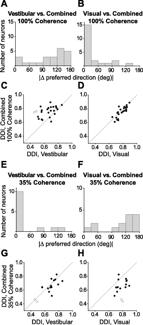
Summary of the differences in direction preference and comparison of tuning strength between the combined and each of the vestibular and visual conditions. A, B, Histograms of the absolute difference in 3D preferred directions (|Δ preferred direction|) between combined (100% coherence) and either the vestibular or the visual condition, respectively (n = 23). C, D, Scatter plots of the DDI for the combined (100% coherence) and either the vestibular or the visual condition, respectively (n = 25). E, F, Histograms of the |Δ preferred direction| between combined (35% coherence) and either the vestibular or the visual condition, respectively (n = 14). G, H, Scatter plots of the DDI for the combined (35% coherence) and either the vestibular or the visual condition, respectively (n = 16). Filled symbols indicate cells for which both the combined and vestibular (C, G) or visual (D, H) tuning was significant (ANOVA, p < 0.05). Open symbols denote cells for which either the combined or the vestibular (C, G)/visual (D, H) tuning was not significant (ANOVA, p > 0.05).
To quantify the variability of responses for each neuron, we calculated the variance/mean ratio or Fano factor (FF). The FF was computed for each of the 26 stimulus directions, and the geometric mean across directions was calculated to obtain a single FF value for each neuron.
To determine whether a measured distribution was significantly different from uniform, we performed a resampling analysis. First, we calculated the sum-squared error (across bins) between the measured distribution and an ideal uniform distribution containing the same number of observations. Next, we generated a random distribution by drawing the same number of data points from a uniform distribution using the “unifrnd” function in Matlab. The sum-squared error was again calculated between this random distribution and the ideal uniform distribution. This second step was repeated 1000 times to generate a distribution of sum-squared error values that represent random deviations from an ideal uniform distribution. If the sum-squared error for the experimentally measured distribution lay outside the 95% confidence interval of values from the randomized distributions, then the measured distribution was considered to be significantly different from uniform (p < 0.05).
To further assess the number of modes in a distribution that was found not to be uniform, a multimodality test based on the kernel density estimate method (Silverman, 1981; Fisher and Marron, 2001) was used. A von Mises function (the circular analog of the normal distribution) was used as the kernel for circular data and a normal distribution for noncircular data. Watson's U2 statistic (Watson, 1961), corrected for grouping (Brown, 1994), was computed as a goodness-of-fit test statistic to obtain a p value through a bootstrapping procedure (Efron, 1979). The test generated two p values, with the first one (puni) for the test of unimodality and the second one (pbi) for the test of bimodality. For example, if puni was <0.05 and pbi was >0.05, unimodality was rejected and the distribution was classified as bimodal. If pbi was also <0.05, this could indicate the existence of more than two modes in the distribution. However, in the current study, this did not occur, and distributions were therefore classified as either unimodal or bimodal when relevant.
We quantified off-line the ability of the animals to suppress their horizontal and vertical vestibulo-ocular reflexes (VORs) and optokinetic (OKN) reflexes by computing mean eye velocity during the middle 1 s of the stimulus period. Supplemental Figure 1 (available at www.jneurosci.org as supplemental material) summarizes these values (±SEM) for the four cardinal movement directions (rotation, yaw and pitch; translation, left/right and up/down). This analysis shows that residual horizontal/vertical eye movements were very small and that animals suppressed at least 98% of their VOR/OKN reflexes. Torsional eye movements were not measured in these experiments.
To quantify the visual and vestibular contributions to the combined-cue response, we estimated a “vestibular gain” and a “visual gain,” defined as the fraction of the vestibular and visual responses of a cell that must be added together to explain the combined tuning. This analysis, which was applied to the 100% coherence data only, was done by fitting the following equation:
where Rx are matrices of mean firing rates for all heading directions; a1 and a2 are the vestibular and visual gains, respectively; and a3 is a constant that accounts for direction-independent differences between the three conditions. We also computed a “gain ratio,” defined as a1/a2. The higher the gain ratio, the higher the vestibular contribution (relative to visual) to the combined response.
To test whether the gain ratio correlated with the relative strength of tuning in the single-cue conditions, we also computed a visual–vestibular ratio (VVR), defined as follows:
 |
where Rmax (vis) and Rmax (ves) are the maximum mean responses in the visual and vestibular conditions, and Rmin (vis) and Rmin (ves) are the minimum mean responses.
Labyrinthectomy.
We investigated whether response selectivity under both the vestibular rotation and translation conditions arises from labyrinthine signals. To accomplish this, we surgically lesioned the vestibular labyrinths bilaterally (all six semicircular canals and otolith organs) in monkeys Z and Q. Each labyrinthectomy was performed by initially drilling through the mastoid air cells to the bony labyrinth (Angelaki et al., 2000; Newlands et al., 2001). After the canals were identified and opened using a fine-cutting burr, the ampullae were destroyed and the utricle and sacculus were removed under direct visualization. Before closing the wound, Gelfoam (Amersham Biosciences, Kalamazoo, MI) soaked in streptomycin solution was placed in the vestibule to eliminate any potentially viable residual neuroepithelium. The efficacy of bilateral labyrinthectomy was confirmed by absent translational and rotational VORs (0.5–2 Hz) that were monitored at regular intervals.
After labyrinthectomy, MSTd responses were collected by sampling from the same set of recording grid locations used before labyrinthectomy, while using identical experimental protocols. Data were collected 2–3 months after the operation. Because we observed no changes in either the evoked eye movements (VOR) or the neural responses over time, data obtained throughout this recording period have been pooled.
Results
We recorded from any MSTd neuron that was spontaneously active or responded to a large-field flickering random-dot stimulus. While animals fixated a central head-fixed target, each well isolated cell (regardless of visual response strength) was tested with either one or both of the 3D rotation and translation protocols, as illustrated in Figure 2. The translation protocol consisted of straight movements along 26 directions (Fig. 2A), corresponding to all combinations of azimuth and elevation angles in increments of 45° (Fig. 2B,C, straight arrows). The rotation protocol consisted of rotations about the same 26 directions (defined according to the right-hand rule) (Fig. 2B,C, curved arrows). Each movement trajectory, either real (vestibular condition) or visually simulated (visual condition), had a duration of 2 s and consisted of a Gaussian velocity profile (Fig. 3) (see also Materials and Methods). Recordings were concentrated in dorsal MST, with recording locations being histologically verified in monkeys Z and Q (Fig. 1).
For the rotation protocol, we recorded from a total of 143 MSTd neurons (74, 27, 5, and 37 from monkeys Q, A, Z, and L, respectively). For the translation protocol, we summarize data from 340 MSTd cells (145, 23, and 172 from monkeys Q, A, and Z, respectively). For 88 neurons (60, 23, and 5 from monkeys Q, A, and Z, respectively), both the rotation and translation protocols were completed. Some, but not all, of the cells tested during translation (255 of 340) were also included in the study of Gu et al. (2006b). These data have been included here for two reasons: (1) to emphasize differences in MSTd neurons between rotation and translation; and (2) for a direct comparison of neural responses before and after bilateral labyrinthectomy (monkeys Q and Z).
Relationship between vestibular and visual tuning
Figure 4 shows a typical example of 3D rotation and translation tuning in MSTd. The 3D directional tuning profile for each stimulus condition is shown as a contour map in which the mean firing rate (represented by color) is plotted as a function of azimuth (abscissa) and elevation (ordinate). Data are shown in four panels, with responses in the left column illustrating the vestibular stimulus condition and responses in the right column illustrating the visual stimulus condition. In the vestibular rotation condition (Fig. 4A), the cell showed strong spatial tuning with a peak response at 91° azimuth and −7° elevation, corresponding roughly to a rotation about the forward axis (i.e., roll rotation, right ear down). When the same set of rotations were simulated using optic flow (visual rotation condition) (Fig. 4B), the peak response of the cell occurred for a rotation axis that was nearly opposite (azimuth, 291°; elevation, −18°; corresponding approximately to a left ear-down roll rotation, with small components of pitch and yaw rotation as well).
Under the vestibular translation condition (Fig. 4C), the example cell was also spatially tuned, with preferred direction at 207° azimuth and −52° elevation, corresponding to a leftward and upward heading. A similar direction preference was seen under the visual translation condition (Fig. 4D), with the peak response occurring at a 190° azimuth and −50° elevation. Note that stimulus directions in both the vestibular and visual conditions are referenced to the actual or simulated motion of the body. Thus, congruent visual/vestibular responses should have the same azimuth/elevation preferences. For the example cell in Figure 4, visual/vestibular preferred directions were congruent for translation but incongruent (oppositely directed) for rotation.
Among all MSTd neurons tested during rotation, 127 of 143 (89%) cells were significantly tuned for direction in the vestibular condition compared with 127 of 128 (99%) cells that were significantly tuned in the visual rotation condition (ANOVA, p < 0.05). Thus, rotational selectivity is quite prevalent in MSTd for both vestibular and visual stimuli. For translation, 183 of 340 (54%) cells were significantly tuned in the vestibular condition, whereas 307 of 318 (97%) cells were significantly tuned for direction of translation in the visual condition (ANOVA, p < 0.05). For both rotation and translation, vestibular responses were usually weaker than the corresponding visual responses (paired t test, p ≪ 0.001). The difference between maximum and minimum responses averaged (±SEM) 27.2 ± 1.3 spikes/s for vestibular rotation and 21.1 ± 1.0 spikes/s for vestibular translation compared with 45.1 ± 2.4 spikes/s for visual rotation and 49.0 ± 1.6 spikes/s for visual translation. Although visual responses are strongest in MSTd, robust vestibular responses are frequently observed.
Notably, all MSTd neurons were characterized by incongruent (nearly opposite) visual and vestibular preferences for rotation, similar to the example neuron in Figure 4. This pervasive incongruency in response to rotational motion stands in contrast to the situation for translational motion, in which visual and vestibular preferences tend to be either congruent or opposite in approximately equal numbers (see also Gu et al., 2006b). These relationships are summarized for all MSTd cells in Figure 5. Distributions of the difference in 3D preferred directions (|Δ preferred direction|) are shown in Figure 5, A and B, where |Δ preferred direction| is computed as the smallest angle between the visual and vestibular direction preferences in three dimensions. For rotation, the distribution of |Δ preferred direction| (Fig. 5A) shows a prominent peak near 180°, indicating that most neurons have nearly opposite preferred directions for vestibular and visual rotation. This distribution is significantly nonuniform (p ≪ 0.001, uniformity test; see Materials and Methods) and clearly unimodal (puni = 0.1, modality test; see Materials and Methods). Strikingly, only 3 of 113 (2.6%) MSTd neurons had visual and vestibular rotation preferences within 90° of each other.
In stark contrast, the distribution of |Δ preferred direction| for translation is clearly bimodal (Fig. 5B), indicating the presence of both congruently and oppositely directed neurons in approximately equal numbers (p ≪ 0.001, uniformity test; puni ≪ 0.001 and pbi = 0.9, modality test) (see also Gu et al., 2006b). To exclude the possibility that these distributions are dominated by neurons with a particular direction preference, we also show the differences between vestibular and visual direction preferences in each cardinal plane: X–Z (front view), Y–Z (side view), and X–Y (top view) (Fig. 5C,D). The pattern of visual/vestibular direction differences seen in three dimensions clearly persists when the difference vectors are projected onto the three cardinal planes [p ≪ 0.001, uniformity test; puni > 0.33, modality test (Fig. 5C); p ≪ 0.001, uniformity test; puni< 0.007 and pbi > 0.13, modality test (Fig. 5D)].
Distribution of preferred directions
The above analysis describes the relative preferences of MSTd neurons for visual and vestibular stimuli but does not specify the distribution of direction preferences across the population. For all neurons with significant spatial tuning (ANOVA, p < 0.05), the direction preference (for rotation and translation, separately) was defined by the azimuth and elevation of the vector average of the neural responses (see Materials and Methods). Figure 6 shows the distributions of direction preferences of all MSTd cells for each of the four stimulus conditions (vestibular rotation, visual rotation, vestibular translation, and visual translation). Each data point in these scatter plots specifies the preferred 3D direction of a single neuron, whereas histograms along the boundaries show the marginal distributions of azimuth and elevation preferences. The distributions of azimuth preferences were significantly bimodal for all four stimulus conditions (p ≪ 0.001, uniformity test; puni < 0.02 and pbi > 0.42, modality test). The distributions of elevation preferences were also significantly bimodal for both of the visual conditions (p ≪ 0.001, uniformity test; puni < 0.004 and pbi > 0.32, modality test). However, the distribution of elevation preferences was not significantly different from uniform for the vestibular rotation condition (p = 0.40, uniformity test) and was just marginally different from uniform for the vestibular translation condition (p = 0.004, uniformity test; puni = 0.12 and pbi = 0.49, modality test).
Figure 6.

Distribution of 3D direction preferences of MSTd neurons, plotted separately for vestibular rotation (A; n = 127), visual rotation (B; n = 127), vestibular translation (C; n = 183), and visual translation (D; n = 307). Each data point in the scatter plot corresponds to the preferred azimuth (abscissa) and elevation (ordinate) of a single neuron with significant tuning (ANOVA, p < 0.05). Histograms along the top and right sides of each scatter plot show the marginal distributions. Also shown are 2D projections (front view, side view, and top view) of unit-length 3D preferred direction vectors (each radial line represents one neuron). The neuron in Figure 4 is represented as open circles in each panel.
For rotation, the peaks of the bimodal azimuth distributions were clearly different in the vestibular and visual conditions (Fig. 6, compare A, B). Vestibular rotation preferences were clustered around azimuths of 90 and 270° [which correspond to roll rotations when elevation is 0° (Fig. 6A)]. In fact, about one-quarter (28%) of MSTd cells had vestibular rotation preferences within 30° of the roll axis (Table 1) [note that distance from the axis is defined in the spherical coordinates of the stimuli (Fig. 2A)]. In contrast, only about one-tenth of MSTd cells had vestibular rotation preferences within 30° of the yaw or pitch axes (Table 1). A complementary pattern was found for the visual rotation condition: preferred azimuths were tightly clustered around 0 and 180° (Fig. 6B), with half of the visual rotation preferences being within 30° of the yaw or pitch axes (Table 1). In contrast, only one MSTd neuron (the cell illustrated in Fig. 4 and marked with open circles in Fig. 6) was found to have a visual rotation preference within 30° of the roll axis (Table 1).
Table 1.
Percentage of neurons with preferred rotation directions within ±30° of each of the cardinal axess
| Rotation | Yaw | Pitch | Roll |
|---|---|---|---|
| Vestibular | 15/127 rotation (12%) | 12/127 rotation (9%) | 36/127 rotation (28%) |
| Visual | 36/127 rotation (28%) | 27/127 rotation (21%) | 1/127 rotation (1%) |
For translation, there was a preference for lateral (azimuths, 0 and 180°) compared with forward/backward directions, and this was true for both the vestibular and visual conditions (Fig. 6C,D) (see also Gu et al., 2006b). Approximately half of the visual and vestibular translation preferences were within 30° of the lateral or vertical axis, with only a handful of neurons having forward/backward preferences (Table 2).
Table 2.
Percentage of neurons with preferred translation directions within ±30° of each of the cardinal axes
| Translation | Lateral | Forward-backward | Vertical |
|---|---|---|---|
| Vestibular | 49/183 translation (27%) | 6/183 translation (3%) | 46/183 translation (25%) |
| Visual | 57/307 translation (19%) | 20/307 translation (7%) | 76/307 translation (25%) |
It is important to emphasize that a dearth of neurons that prefer motion along a particular axis does not necessarily imply that few cells respond to this stimulus. To illustrate this point, we examined whether the firing rate along each of the six cardinal directions on the sphere differed significantly from spontaneous activity. The percentages of neurons showing significant activation for each axis, along with the mean (±SEM) evoked responses across the population (maximum response − spontaneous activity), are summarized in Tables 3 and 4. The percentage of MSTd neurons that responded significantly to motion along (or about) each axis was similar (∼30–60%) for all cardinal directions. Notably, although few MSTd neurons preferred roll rotation in the visual condition, the mean evoked response around the roll axis was comparable to that for the other rotation axes (Table 3). Moreover, nearly half of MSTd neurons showed significant evoked responses (relative to spontaneous activity) during roll visual stimulation. This occurs mainly because the spatial tuning of most MSTd neurons is quite broad, often approximating cosine tuning (Fig. 4) (see also Gu et al., 2006b). Indeed, it is worth emphasizing that neurons operating around the steep slope of their tuning curve will provide the most information for discrimination of motion direction (Bradley et al., 1987; Osborne et al., 2004; Purushothaman and Bradley, 2005). Thus, the lack of neurons tuned to roll rotation in the visual condition (Fig. 6B) does not imply a lack of information about roll movements.
Table 3.
Summary of responses to rotation about each of the cardinal axes
| Rotation | Yaw |
Pitch |
Roll |
|||
|---|---|---|---|---|---|---|
| Left | Right | Up | Down | Clockwise | Counterclockwise | |
| Vestibular | 59/143 (41%) | 50/143 (35%) | 53/143 (37%) | 50/143 (35%) | 63/143 (44%) | 66/143 (46%) |
| Max-spont (±SEM) | 5.1 (±2.5) | 5.3 (±2.4) | 5.7 (±2.4) | 5.0 (±2.6) | 6.6 (±2.5) | 7.5 (±2.6) |
| Visual | 73/128 (57%) | 69/128 (54%) | 73/128 (57%) | 74/128 (58%) | 73/128 (57%) | 69/128 (54%) |
| Max-spont (±SEM) | 6.3 (±2.3) | 6.1 (±2.3) | 7.1 (±2.2) | 8.5 (±2.3) | 6.5 (±2.3) | 6.7 (±2.4) |
Data shown represent either percentage of neurons with significant responses compared with spontaneous activity (top) or mean (±SEM) evoked response [maximum–spontaneous activity (Max-spont)], computed for all cells.
Table 4.
Summary of responses to translation along each of the cardinal axes
| Translation | Lateral |
Fore-aft |
Vertical |
|||
|---|---|---|---|---|---|---|
| Left | Right | Forward | Backward | Up | Down | |
| Vestibular | 111/340 (33%) | 104/340 (31%) | 99/340 (29%) | 90/340 (26%) | 108/340 (32%) | 100/340 (29%) |
| Max-spont (±SEM) | 5.8 (±2.8) | 5.4 (±2.6) | 4.6 (±2.7) | 4.4 (±2.8) | 5.0 (±2.7) | 5.6 (±2.9) |
| Visual | 176/318 (55%) | 157/318 (49%) | 153/318 (48%) | 155/318 (49%) | 143/318 (45%) | 164/318 (52%) |
| Max-spont (±SEM) | 10.3 (±2.8) | 8.6 (±2.6) | 7.8 (±2.7) | 8.0 (±2.9) | 7.5 (±2.5) | 10.8 (±2.8) |
Data shown represent either percentage of neurons with significant responses compared with spontaneous activity (top) or mean (±SEM) evoked response [maximum–spontaneous activity (Max-spont)], computed for all cells.
Relationship between rotation and translation tuning
Thus far, we have examined visual and vestibular selectivity for translation and rotation separately. In addition, a subset of MSTd cells was tested with both the rotation and translation protocols, thus allowing a direct comparison between rotation and translation tuning. Overall, vestibular rotation tuning was significantly stronger (mean DDI, 0.66 ± 0.01 SEM) than vestibular translation tuning (mean DDI, 0.56 ± 0.01 SEM) (paired t test, p ≪ 0.001; n = 88) (Fig. 7A). However, the reverse was true for the visual condition, where translation selectivity (mean DDI, 0.82 ± 0.01 SEM) was slightly stronger than rotation selectivity (mean DDI, 0.78 ± 0.01 SEM) (paired t test, p < 0.001; n = 63) (Fig. 7B).
Forty-eight neurons (55%) were significantly tuned for both translation and rotation in the vestibular condition (ANOVA, p < 0.05) (Fig. 7A). The distribution of the difference in 3D direction preference (|Δ preferred direction|) between vestibular rotation and vestibular translation is shown in Figure 7C. Although there is some tendency for vestibular translation and rotation preferences to differ by ∼90°, this distribution was not significantly different from uniform (uniformity test, p = 0.09). The corresponding distribution of directional differences between the visual rotation and translation conditions is shown in Figure 7D [97% of MSTd neurons (61 of 63) showed significant tuning for both types of visual stimuli (Fig. 7B)]. In this case, the distribution is strongly nonuniform (uniformity test, p ≪ 0.001), with a clear mode near 90°. This relationship is sensible when one considers the structure of the visual stimulus that drives MSTd neurons. Specifically, visual translation and rotation preferences are typically linked by the two-dimensional (2D) visual motion selectivity of the cell. For example, an MSTd neuron that prefers downward visual motion on the display screen will respond well to both an upward pitch stimulus (azimuth, 0°; elevation, 0°) and a vertical (upward) translation stimulus (azimuth, 0°; elevation, −90°). Note that these two stimulus directions are 90° apart on the sphere (Fig. 2). This is typical of the results presented in Figure 7D.
Because |Δ preferred direction| is computed as the smallest angle between a pair of preferred direction vectors in three dimensions, it is only defined within the interval of (0, 180°). Thus, it is important to further examine whether the observed peak near 90° in Figure 7D is derived from a single mode at −90° or from two modes at +90 and −90°. Only the former condition (but not the latter) would show that visual preferences for translation and rotation are linked via the 2D visual motion selectivity of the cell. To examine this, we also illustrate the differences between translation and rotation preferences in each cardinal plane: X–Z (front view), Y–Z (side view), and X–Y (top view) (Fig. 7E, F). The advantage of this approach is that we can plot the directional differences over the entire 360° range. To compute these directional differences within the cardinal planes, each 3D preference vector was projected onto the plane of interest, and the angle between these projections was measured. Because some planar projections might be small in amplitude, we also calculated the ratio of the lengths of each difference vector in two and three dimensions. These vector length ratios are plotted against the 2D preferred direction difference in Figure 7, G and H.
Because few MSTd neurons had a strong visual rotation component along the roll axis, the projections of the visual difference vector onto the Y–Z and X–Y planes were relatively small (Fig. 7H, green and blue data points). In contrast, the projection of the visual difference vector onto the X–Z plane was substantially larger (Fig. 7H, red data points) (ANOVA, p ≪ 0.001). As a result, the distribution of 2D direction differences in the frontal (X–Z) plane is more revealing than those in the other two planes (Fig. 7F, red vs green and blue histograms). The frontal (X–Z) plane distribution is tightly centered at −90°, with no cells having direction differences of +90° between visual translation and rotation. Thus, the data from the visual condition are mostly consistent with the idea that the preferred directions for translation and rotation are related through the 2D visual motion selectivity of the neurons.
It is important to emphasize that our visual stimuli contained sufficient cues to allow one to distinguish between simulated rotation and translation, even when both produced flow fields with a dominant laminar flow component (e.g., horizontal or vertical 2D visual motion). Because our visual stimulus simulated motion of the observer through a 3D volume of dots, our rotation and translation stimuli differed both in motion parallax and binocular disparity. Yet, MSTd neurons generally gave similar responses to rotations and translations that produced the same overall direction of 2D visual motion (Fig. 7B, D). Given that simulated rotations and translations produce flow fields with somewhat different distributions of speeds and disparities of individual dots, as well as the fact that we did not quantify the speed and disparity tuning of our MSTd neurons, it is difficult to quantitatively compare responses produced by visual translation and rotation stimuli. However, the general similarity of responses under these two conditions is consistent with the notion that these cells might not discriminate self-rotation from self-translation based on optic flow alone (see Discussion). Unlike the visual stimulus condition, differences in direction preference between translation and rotation for the vestibular condition were not tightly distributed in any of the cardinal planes (Fig. 7E, G).
The tuning of MSTd neurons in the vestibular condition could arise from labyrinthine vestibular signals or from other nonvisual (e.g., somatosensory) cues. To investigate the role of labyrinthine signals in driving MSTd responses, we performed two control experiments. First, we compared how firing rates changed in the vestibular condition when rotation occurred in total darkness rather than during fixation of a head-fixed target. Second, we also recorded from MSTd neurons after bilateral labyrinthectomy. In the following two sections, we describe each of these experiments.
Comparison of responses in darkness versus fixation
A subpopulation of MSTd neurons (n = 34) was tested during 3D rotation in complete darkness (with the projector turned off; see Materials and Methods). Figure 8A shows the vestibular rotation tuning of one of these cells during fixation. It has a preferred vestibular rotation axis at a 4° azimuth and 17° elevation, corresponding approximately to pitch-up motion (Fig. 8A). The preferred rotation axis in the visual condition was oriented in the opposite direction: at an azimuth of 176° and an elevation of −18° (simulating pitch-down motion) (Fig. 8B). Rotation tuning during vestibular stimulation in complete darkness was quite similar to that obtained during the fixation protocol (Fig. 8, compare A, C). However, responses were a bit weaker in darkness, as illustrated by the reduced amplitude of the peristimulus time histograms of the neural responses along one of the motion directions (azimuth, 0°; elevation, 0°) in Figure 8D.
We found that 23 of 34 neurons tested (all of which were significantly tuned to vestibular rotation during fixation) were also significantly tuned during rotation in darkness (ANOVA, p < 0.05). Figure 9A plots the distribution of the absolute difference in 3D direction preference between fixation and darkness. With the exception of two cells, MSTd neurons tended to have similar direction preferences in the fixation and darkness protocols, with a median difference of 27.9°. Similarly, the difference between maximum and minimum response amplitude (Rmax − Rmin) during rotation in darkness was not significantly different from that observed during fixation (paired t test, p = 0.13), as shown in Figure 9B. Tuning strength, as measured with a DDI (see Materials and Methods), was significantly lower in darkness than during fixation (paired t test, p = 0.009), as shown in Figure 9C. Together, Figure 9, B and C, suggests that the variability of MSTd responses to rotation was larger in darkness than during fixation. Indeed, this was confirmed by the finding of a significantly larger variance/mean ratio (i.e., FF) under darkness (2.38 ± 0.21 SEM) compared with during fixation (1.28 ± 0.11 SEM) (paired t test, p ≪ 0.001). Thus, MSTd responses to vestibular rotation stimuli appear to be more variable in darkness than during fixation (perhaps because of unconstrained movements of the eyes), but the tuning profile for rotation is quite well preserved.
A similar comparison between fixation and darkness has been made previously for translational movements (Gu et al., 2006b). For translation, there was even less difference between fixation and darkness, indicating that neither form of directional selectivity depends on active fixation (and consequent cancellation of VORs). In the following presentation of data from labyrinthectomized animals, we focus our quantitative analyses on vestibular responses during fixation (because this condition could be interleaved with the visual stimulus condition).
Strength of visual and vestibular tuning: effects of bilateral labyrinthectomy
To further investigate the role of labyrinthine signals in driving responses of MSTd neurons, we recorded from 81 MSTd neurons (23 and 58 from monkeys Q and Z, respectively) under the rotational protocol and 79 cells (26 and 53 from monkeys Q and Z, respectively) under the translational protocol after bilateral labyrinthectomy. Only a handful of MSTd neurons in labyrinthectomized animals (1 of 81 cells for rotation and 3 of 79 cells for translation) showed significant direction tuning in the vestibular condition (ANOVA, p < 0.05). The proportion of neurons with significant tuning after labyrinthectomy did not exceed chance. In contrast, all MSTd cells in labyrinthectomized animals were significantly tuned to visual rotation and/or translation (ANOVA, p < 0.05).
These observations are summarized in Figure 10, A and B, which plots the DDI for the visual condition (ordinate) against the corresponding DDI for the vestibular condition (abscissa). Red and blue data points indicate results obtained before and after bilateral labyrinthectomy, respectively. Filled symbols indicate neurons with significant directional selectivity in both the vestibular and visual conditions; open symbols denote cells without significant vestibular tuning. Vestibular DDI values were significantly smaller in labyrinthectomized animals (blue symbols) compared with labyrinthine-intact animals (red symbols) (ANOVA, p ≪ 0.001). This was true for both the vestibular rotation and vestibular translation conditions. The rotation effects appear to be larger, but this is because the average DDI for translation in labyrinthine-intact animals is significantly smaller than that for rotation (paired t test, p ≪ 0.001) (Fig. 7A).
Figure 10.
Comparison of tuning strength and response amplitude between visual and vestibular conditions before and after bilateral labyrinthectomy. A, B, Tuning strength is quantified by the DDI and is plotted separately for rotation and translation protocols. C, D, Scatter plots of response amplitude (Rmax − Rmin). Filled symbols indicate cells for which both visual and vestibular tuning was significant (ANOVA, p < 0.05); open symbols denote cells without significant vestibular tuning (ANOVA, p > 0.05). Histograms along the top and right sides of each scatter plot show the marginal distributions (including both open and filled symbols). Red symbols and bars denote data from labyrinthine-intact (normal) animals; blue symbols and bars denote data from labyrinthectomized animals.
In contrast to the significant differences in vestibular DDIs before and after labyrinthectomy, no such difference was seen for DDIs from the visual condition (ANOVA, p = 0.75 for visual rotation and p = 0.13 for visual translation) (see marginal distributions in Fig. 10A,B). The latter result rules out the possibility of a nonspecific effect of labyrinthectomy on responsiveness of MSTd neurons. Similar conclusions were also made when comparing firing rate modulations (Rmax − Rmin) (Fig. 10C,D) rather than DDI values. Thus, the signals responsible for MSTd responses to rotation and translation in the absence of optic flow appear to arise almost exclusively from the vestibular labyrinths.
Contribution of vestibular signals during cue combination
For translation, adding optic flow to inertial motion results in selectivity that is typically similar to that seen in the visual condition (Gu et al., 2006b). At 100% motion coherence, visual responses in MSTd are stronger than the corresponding vestibular responses to translation, such that the latter contribute relatively little to the combined response (Gu et al., 2006b). However, this visual dominance of heading tuning might be attributable to the fact that the visual stimulus, at 100% coherence, is more reliable than the vestibular stimulus. Indeed, our preliminary results for translation (Gu et al., 2006a) suggest that visual and vestibular signals may interact more strongly when the motion coherence of the visual stimulus is reduced.
To examine this possibility for rotation, we tested a subpopulation of 23 MSTd cells from monkey L with a combined visual/vestibular stimulus at both high and low motion coherences (see Materials and Methods). Figure 11 shows results from four representative neurons. The cells in Figure 11, A and B, like the majority of MSTd neurons (Fig. 10A, C), had stronger visual than vestibular tuning. When the two cues were combined at 100% motion coherence, the visual response dominated for these two neurons. For example, the combined response of the cell in Figure 11A (third row) had a peak at 4° azimuth and 17° elevation (similar to the visual preference of 331° azimuth and 15° elevation). Note that the vestibular signals also contributed to a secondary peak in the combined response. In contrast, when visual motion coherence was reduced to 35%, the vestibular peak became dominant in the combined response (Fig. 11A, fourth row) (peak at 124° azimuth and −28° elevation, similar to the vestibular preference of 133° azimuth and −23° elevation). In contrast, the visual peak was greatly reduced at low coherence. Similar observations apply to the cell in Figure 11B.
For some MSTd cells that had similar tuning strengths in the vestibular and visual conditions (Fig. 11C,D), either the vestibular or the visual cues could dominate the combined response. When the stimuli were combined at high motion coherence, the visual peak was dominant (and the vestibular response was suppressed) for the cell in Figure 11C, whereas the vestibular peak was dominant (and the visual response was suppressed) for the cell in Figure 11D (third row). When visual coherence was reduced to 35%, spatial tuning was similar to the vestibular tuning in both neurons (Fig. 11C,D, fourth row vs first row).
To summarize these results, we compare the DDI and the direction preference in the combined condition with the corresponding values for the vestibular and visual conditions (Fig. 12). At 100% motion coherence, only 22% (5 of 23) of the neurons had a combined rotation preference that was within 60° of the vestibular preference, whereas 78% (18 of 23) of the neurons had a combined preference within 60° of the visual preference (Fig. 12A, B). Thus, at high coherence, rotation preferences in the combined condition were dominated by visual input, as we previously found for translation (Gu et al., 2006b). This pattern reversed when motion coherence was reduced to 35%: now 79% (11 of 14) of the cells had a combined preference within 60° of the vestibular preference, whereas 21% (3 of 14) were closer to the visual preference (Fig. 12E, F).
Regarding tuning strength, the DDI in the combined condition (at 100% motion coherence) was significantly larger than the corresponding vestibular DDI (paired t test, p ≪ 0.001) (Fig. 12C). At 35% coherence, the combined DDI was not significantly different from the vestibular DDI (paired t test, p = 0.24) (Fig. 12G). Importantly, for both motion coherence levels, the combined DDI was significantly lower than the corresponding visual DDI [paired t test, p = 0.014 (Fig. 12D); paired t test, p ≪ 0.001 (Fig. 12H)]. Thus, adding inertial motion significantly reduced the spatial selectivity of MSTd neurons in the visual condition. This result is not surprising given that all MSTd neurons have incongruent visual and vestibular preferences during rotation (Fig. 5A).
To further evaluate the vestibular contribution to the combined response, for 23 neurons with significant tuning under both single-cue conditions, we computed vestibular and visual gains, as well as their ratio (gain ratio; see Materials and Methods). These gains describe the weighting of the visual and vestibular responses that provide the best linear fit to the combined response. Figure 13A shows a plot of the visual rotation gain against the vestibular rotation gain. There is a slight trend for these gains to be anticorrelated, but this trend did not reach significance (r = −0.01; p = 0.9, Spearman rank correlation). We also performed the same analysis on the much larger set of translation data, and the corresponding scatter plot is shown in Figure 13B. Here, the anticorrelation of the gains was more significant (r = −0.21; p = 0.02, Spearman rank correlation).
Figure 13.
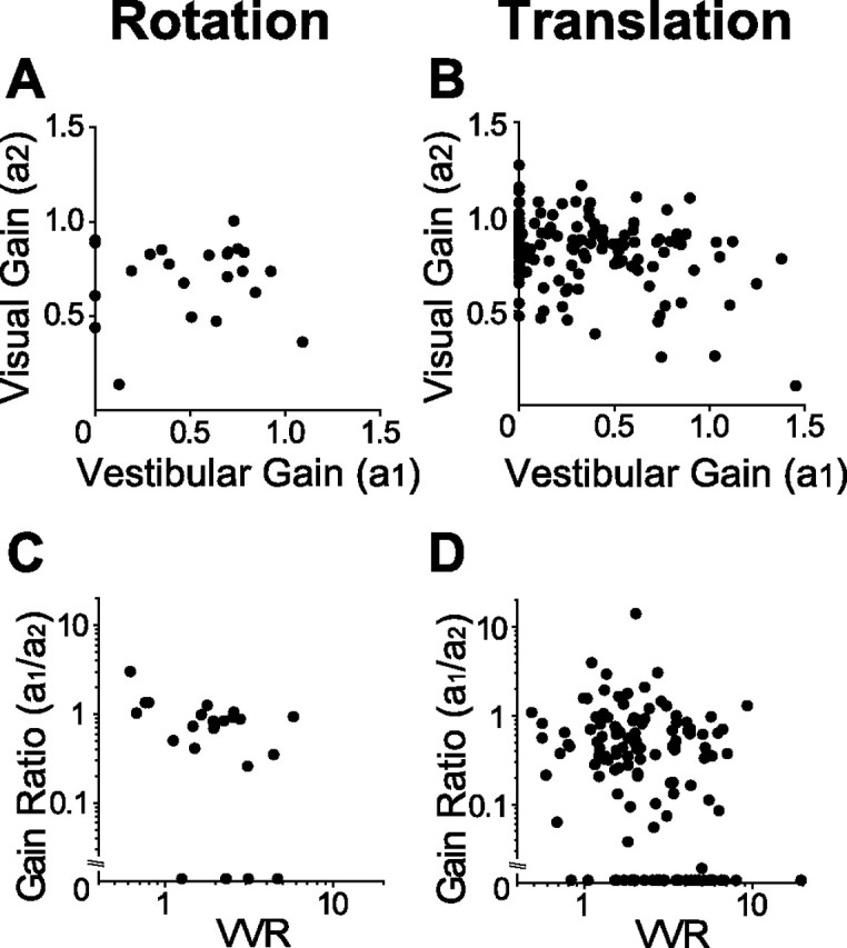
Quantification of vestibular and visual contributions to the combined response for both the rotation and translation protocols. A, B, Relationship between vestibular gain (a1) and visual gain (a2). C, D, Gain ratio (a1/a2) plotted as a function of relative tuning strength between visual and vestibular responses (VVR). Number of neurons: n = 23 (A, C); n = 133 (B, D).
Figure 13, C and D, plots the vestibular/visual gain ratio (a1/a2) as a function of the relative strength of selectivity measured in the visual and vestibular conditions. A gain ratio of 1 indicates that vestibular and visual cues are equally weighted in the combined response. In contrast, a gain ratio of 0 suggests that vestibular responses make no contribution to the combined tuning, and a gain ratio >1 means that vestibular cues outweigh the visual cues. The relative tuning strength for the two single cues is characterized by the VVR (VVR >1 indicates that tuning strength was stronger for the visual than the vestibular condition; see Materials and Methods). We find a significant negative correlation between the gain ratio and VVR for both rotation (r = −0.45; p = 0.03, Spearman rank correlation) (Fig. 13C) and translation (r = −0.31; p ≪ 0.001, Spearmann rank correlation) (Fig. 13D). This indicates that the relative strength of tuning for the two cues, tested separately, is predictive of how the cues interact to determine the combined response. Neurons with stronger vestibular tuning have a greater vestibular contribution to the combined response.
The mean gain ratio (at 100% motion coherence) across the population was 1.14.±2.75 (SD) for rotation (n = 23) compared with 0.49 ± 1.33 (SD) for translation (n = 133). Notably, 17% (4 of 23) of MSTd cells had gain ratios >1 for rotation (suggesting vestibular dominance), but only 9% (12 of 133) had gain ratios >1 for translation. Thus, vestibular cues tend to contribute more strongly to combined responses during rotation than during translation.
Discussion
Area MSTd lies within extrastriate visual cortex and is not typically considered to be a part of “vestibular cortex,” which is thought to include the parieto-insular vestibular cortex, area 2v, and area 3a (Schwarz and Fredrickson, 1971; Akbarian et al., 1988; Fukushima, 1997). Yet, we have shown that MSTd responses during physical movement in the absence of optic flow arise from sensory signals originating in the vestibular labyrinths. In response to vestibular stimuli, the percentage of MSTd neurons that were spatially tuned for rotation was significantly higher than that for translation. Thus, although MSTd has often been considered as a neural substrate for heading perception during translational motion (Duffy and Wurtz, 1995; Lappe et al., 1996; Britten and van Wezel, 1998; Duffy, 1998), rotational selectivity is also abundant in MSTd. The anatomical pathways that deliver vestibular information to MSTd still remain to be determined, however.
Preferred directions for rotation were distributed throughout 3D space, with most cells preferring roll motion in the vestibular condition and pitch/yaw motion in the visual condition. As a result, visual and vestibular rotation preferences were never congruent, with preferred directions typically lying 120–180° apart (Fig. 5A). This incongruency of visual and vestibular rotation preferences contrasts sharply with the equal presence of congruent and opposite preferences for translation (Fig. 5B) (see also Gu et al., 2006b). These observations suggest that the roles of MSTd in self-motion perception may be different for translation and rotation, as discussed further below.
Tuning of MSTd neurons for visual rotation and translation
A traditional approach to describing optic flow selectivity in MSTd has involved characterizing responses to “planar” (horizontal/vertical), “radial” (expansion/contraction), and “circular” (clockwise/counterclockwise) components of optic flow. Whereas some MSTd neurons respond to only one of these components, the majority exhibit selectivity for multiple components (Saito et al., 1986; Tanaka et al., 1986; Tanaka and Saito, 1989; Duffy and Wurtz, 1991; Lagae et al., 1994; Geesaman and Andersen, 1996; Heuer and Britten, 2004), often resulting in a continuous sampling of spiral space [i.e., combinations of expansion/contraction and clockwise/counterclockwise rotation (Orban et al., 1992; Graziano et al., 1994; Duffy and Wurtz, 1997)].
Our approach to defining the space of optic flow stimuli differs in multiple respects from previous studies. Rather than simulating self-motion relative to a fronto-parallel plane (i.e., a wall), we instead simulate motion through a virtual 3D volume of random dots. This produces naturalistic visual stimuli replete with binocular disparity, motion parallax, and texture cues. We parameterize the stimuli according to the subject's simulated direction of translation or rotation in three dimensions. Accordingly, we characterize neural responses to optic flow in terms of simulated 3D self-motion, not in terms of the 2D pattern of visual motion generated on the display (although the two are related). For example, either a simulated rightward translation or a simulated rightward yaw rotation will produce a laminar optic flow field in which all dots move leftward on the screen. Notably, however, the dynamic changes in texture, motion parallax, and binocular disparity that are available in our stimuli can allow one to distinguish between a horizontal self-rotation and a horizontal self-translation.
Despite differences in approach, our results are generally compatible with those of previous studies (Graziano et al., 1994; Duffy and Wurtz, 1997; Heuer and Britten, 2004). We found a continuous coding of both visual rotation and visual translation directions, although the direction preferences were not distributed uniformly or unimodally. In particular, there was a paucity of visual preferences for roll rotation and a predominance of preferences for pitch and yaw rotations (Fig. 6B). Visual preferences for translation were strongly biased in favor of lateral as compared with forward/backward movements (Fig. 6D) (see also Gu et al., 2006b) (but see Logan and Duffy, 2006). Despite these biased distributions of direction preference, the percentage of neurons that were significantly activated (relative to spontaneous activity) was fairly uniform across directions, varying between 26 and 58% for all cardinal motion directions (Tables 3, 4). Although few MSTd neurons preferred roll rotation in optic flow, many neurons responded to this stimulus (because tuning is broad) and would be capable of discriminating changes in rotation axis around the roll direction.
We found a tight relationship between visual preferences for rotation and translation (Fig. 7D). For example, if a cell preferred upward pitch rotation, it also preferred upward translation, because both stimuli produce downward visual motion on the display screen. Because of our conventions for defining translation and rotation, this produces a tight clustering of directional differences around −90° (Fig. 7D,F). This observation suggests that the visual responses of most MSTd neurons to 3D rotations and translations may be predictable based on the direction of 2D visual motion that the neuron prefers within its receptive field. This would be consistent with the conspicuous absence of cells that have visual preferences for roll rotation and the relatively small proportion of cells that prefer forward or backward translation (radial flow). This linkage between 3D direction preference and 2D visual motion preference may be a reflection of the inputs from area MT, which are generally thought to represent 2D visual motion rather than motion in depth (Maunsell and van Essen, 1983) (but see Xiao et al., 1997).
Although our visual stimuli contained sufficient cues to distinguish between 3D translation and rotation, most MSTd neurons produced similar peak responses to these two sets of stimuli (Fig. 4). This raises the question of whether a population of MSTd neurons can distinguish between self-rotation and self-translation based solely on optic flow. Our data do not allow a definitive analysis of this issue because the translation and rotation stimuli have different spatiotemporal distributions of retinal speeds and disparities, and because we have not measured the local selectivity of the neurons for speed and disparity. Nevertheless, this issue deserves attention in future studies.
Tuning of MSTd neurons for vestibular rotation and translation
In addition to measuring optic flow selectivity using naturalistic stimuli, an advantage of our approach is that we also characterize MSTd responses during physical motion of the subject in the absence of optic flow. Approximately half of the neurons showed significant vestibular tuning for translation (see also Gu et al., 2006b), but nearly all (89%) MSTd cells exhibited significant vestibular tuning for rotation.
There are at least two main possibilities regarding the origin of these nonvisual responses in MSTd. First, they might represent sensory vestibular signals that are independent of oculomotor behavior. If so, then vestibular tuning should be identical during fixation of a head-fixed target and during unconstrained viewing in complete darkness. Alternatively, vestibular tuning in MSTd might be generated because the animal actively suppresses his horizontal/vertical VOR during fixation of a head-fixed target. This is plausible given that the majority of MST neurons are known to modulate during horizontal/vertical smooth pursuit and ocular following (Komatsu and Wurtz, 1988a,b; Newsome et al., 1988; Kawano et al., 1994). To address this important issue, we compared vestibular rotation tuning measured during free viewing in darkness with tuning measured during fixation (Figs. 8, 9), and we found only small differences in rotation selectivity between the two conditions. Direction preferences were generally well matched (Fig. 9A), and response strengths were also similar (Fig. 9B). The only substantial difference was that response variability was higher (and DDI thus lower) in darkness, presumably because the uncontrolled eye movements of the animal might modulate MSTd responses. We previously made a similar comparison for vestibular responses to translation (Gu et al., 2006b) and found similar (if not smaller) effects. Thus, vestibular selectivity for rotation and translation in MSTd appears not to be merely a byproduct of VOR suppression.
Unlike in the visual stimulus condition, differences in direction preference between translation and rotation for the vestibular condition were not tightly clustered around −90°. Such clustering would be expected if, like in the visual condition, rotational and translational responses were of a common origin. This could occur if rotational responses in MSTd were at least partly attributable to activation of otolith afferents that do not discriminate between linear accelerations that result from translation and head orientation relative to gravity (Fernandez and Goldberg, 1976a,b,c; Angelaki, 2004; Angelaki et al., 2004). Although some MSTd cells show differences in direction preference between rotation and translation that are close to −90°, many other cells do not. This result suggests that vestibular rotation responses in MSTd are at least partly driven by activation of the semicircular canals. Whether gravity-sensitive, otolith-driven responses also contribute [as in brainstem and cerebellar neurons (Dickman and Angelaki, 2002; Angelaki et al., 2004)] remains to be investigated in future studies.
Relationship between visual and vestibular responses
Visual and vestibular translation preferences of MSTd neurons tended to be either the same (i.e., congruent) or the opposite (Fig. 5B) (see also Gu et al., 2006b). In contrast, visual and vestibular rotation preferences were never congruent and tended to be near opposite (Fig. 5A, C). What might be the functional significance of these patterns of congruency? Neurons with congruent visual and vestibular preferences will be maximally activated during self-motion under natural conditions when both sensory cues are present. In contrast, neurons with incongruent preferences (oppositely directed cells) will not be maximally activated during self-motion through a static visual scene. Using a heading discrimination task, we have reported preliminary evidence that congruent and incongruent MSTd neurons play different roles in perception of self-translation (DeAngelis et al., 2006; Gu et al., 2006a). Specifically, we found that congruent cells showed a greater capacity to discriminate small changes in heading when both visual and vestibular cues are present. A similar improvement in discrimination performance was seen in the monkeys' behavior. In contrast, MSTd neurons with opposite visual and vestibular preferences became less sensitive in the presence of both cues (DeAngelis et al., 2006; Gu et al., 2006a).
These preliminary results for heading (translation) discrimination suggest that congruent cells may contribute to cue integration for robust perception, whereas opposite cells may not. The fact that opposite cells may be maximally activated when visual and vestibular cues are placed in conflict raises the possibility that these neurons play a role in identifying situations in which visual and vestibular stimuli are not consistent with the observer's self-motion. This will arise, for example, whenever the observer moves through an environment in which objects move independently. It is thus possible that opposite cells might be functionally relevant for decomposing retinal image motion into object motion versus self-motion.
The activity of MSTd neurons during rotation discrimination tasks has not been measured. However, because all MSTd cells had oppositely directed visual and vestibular preferences for rotation (Fig. 5A), it seems unlikely that MSTd could account for improved sensitivity in perception of self-rotation when visual and vestibular cues are both present. Our results in the combined rotation condition, in which addition of vestibular cues decreased tuning strength to optic flow (Figs. 11–13), also support this hypothesis. What, then, might be the function of vestibular rotation signals in MSTd? One obvious role would be to disambiguate optic flow that is produced by self-translation from that produced by eye/head/body rotation. Psychophysical studies have shown that human observers can discount both eye rotations (Royden et al., 1992; Banks et al., 1996) and head rotations (Crowell et al., 1998) during judgments of heading. Physiological studies have shown that MSTd neurons can signal heading from optic flow in the presence of pursuit eye movements (Bradley et al., 1996; Page and Duffy, 1999; Shenoy et al., 1999). By analogy, we propose that vestibular rotation signals in MSTd may be involved in compensating for the effects of head rotations on processing of optic flow. In this scenario, MSTd would be involved in the integration of visual and vestibular cues for translation perception but not for rotation perception. This hypothesis is consistent with the fact that mainly translational components of optic flow are used for navigation; rotational optic flow is typically nulled by a compensatory VOR (Angelaki and Hess, 2005). Additional studies will be necessary to test this hypothesis.
Footnotes
This work was supported by National Institutes of Health Grants R01 EY017866, EY016178, and DC04260. We thank Amanda Turner and Erin White for excellent help with animal care and training.
References
- Akbarian S, Berndl K, Grusser OJ, Guldin W, Pause M, Schreiter U. Responses of single neurons in the parietoinsular vestibular cortex of primates. Ann NY Acad Sci. 1988;545:187–202. doi: 10.1111/j.1749-6632.1988.tb19564.x. [DOI] [PubMed] [Google Scholar]
- Angelaki DE. Eyes on target: what neurons must do for the vestibuloocular reflex during linear motion. J Neurophysiol. 2004;92:20–35. doi: 10.1152/jn.00047.2004. [DOI] [PubMed] [Google Scholar]
- Angelaki DE, Hess BJ. Self-motion-induced eye movements: effects on visual acuity and navigation. Nat Rev Neurosci. 2005;6:966–976. doi: 10.1038/nrn1804. [DOI] [PubMed] [Google Scholar]
- Angelaki DE, Newlands SD, Dickman JD. Primate translational vestibuloocular reflexes IV. Changes after unilateral labyrinthectomy. J Neurophysiol. 2000;83:3005–3018. doi: 10.1152/jn.2000.83.5.3005. [DOI] [PubMed] [Google Scholar]
- Angelaki DE, Shaikh AG, Green AM, Dickman JD. Neurons compute internal models of the physical laws of motion. Nature. 2004;430:560–564. doi: 10.1038/nature02754. [DOI] [PubMed] [Google Scholar]
- Banks MS, Ehrlich SM, Backus BT, Crowell JA. Estimating heading during real and simulated eye movements. Vision Res. 1996;36:431–443. doi: 10.1016/0042-6989(95)00122-0. [DOI] [PubMed] [Google Scholar]
- Bertin RJ, Berthoz A. Visuo-vestibular interaction in the reconstruction of travelled trajectories. Exp Brain Res. 2004;154:11–21. doi: 10.1007/s00221-003-1524-3. [DOI] [PubMed] [Google Scholar]
- Bradley A, Skottun BC, Ohzawa I, Sclar G, Freeman RD. Visual orientation and spatial frequency discrimination: a comparison of single neurons and behavior. J Neurophysiol. 1987;57:755–772. doi: 10.1152/jn.1987.57.3.755. [DOI] [PubMed] [Google Scholar]
- Bradley DC, Maxwell M, Andersen RA, Banks MS, Shenoy KV. Mechanisms of heading perception in primate visual cortex. Science. 1996;273:1544–1547. doi: 10.1126/science.273.5281.1544. [DOI] [PubMed] [Google Scholar]
- Bremmer F, Kubischik M, Pekel M, Lappe M, Hoffmann KP. Linear vestibular self-motion signals in monkey medial superior temporal area. Ann NY Acad Sci. 1999;871:272–281. doi: 10.1111/j.1749-6632.1999.tb09191.x. [DOI] [PubMed] [Google Scholar]
- Britten KH, van Wezel RJ. Electrical microstimulation of cortical area MST biases heading perception in monkeys. Nat Neurosci. 1998;1:59–63. doi: 10.1038/259. [DOI] [PubMed] [Google Scholar]
- Brown BM. Grouping corrections for circular goodness-of-fit tests. J R Stat Soc B. 1994;56:275–283. [Google Scholar]
- Crowell JA, Banks MS, Shenoy KV, Andersen RA. Visual self-motion perception during head turns. Nat Neurosci. 1998;1:732–737. doi: 10.1038/3732. [DOI] [PubMed] [Google Scholar]
- DeAngelis GC, Uka T. Coding of horizontal disparity and velocity by MT neurons in the alert macaque. J Neurophysiol. 2003;89:1094–1111. doi: 10.1152/jn.00717.2002. [DOI] [PubMed] [Google Scholar]
- DeAngelis GC, Gu Y, Angelaki DE. Role of area MSTd in cue integration for heading discrimination: II. Analysis of correlations between neural responses and perceptual decisions. J Vision. 2006;6:408a. [Google Scholar]
- Dickman JD, Angelaki DE. Vestibular convergence patterns in vestibular nuclei neurons of alert primates. J Neurophysiol. 2002;88:3518–3533. doi: 10.1152/jn.00518.2002. [DOI] [PubMed] [Google Scholar]
- Duffy CJ. MST neurons respond to optic flow and translational movement. J Neurophysiol. 1998;80:1816–1827. doi: 10.1152/jn.1998.80.4.1816. [DOI] [PubMed] [Google Scholar]
- Duffy CJ, Wurtz RH. Sensitivity of MST neurons to optic flow stimuli. I. A continuum of response selectivity to large-field stimuli. J Neurophysiol. 1991;65:1329–1345. doi: 10.1152/jn.1991.65.6.1329. [DOI] [PubMed] [Google Scholar]
- Duffy CJ, Wurtz RH. Response of monkey MST neurons to optic flow stimuli with shifted centers of motion. J Neurosci. 1995;15:5192–5208. doi: 10.1523/JNEUROSCI.15-07-05192.1995. [DOI] [PMC free article] [PubMed] [Google Scholar]
- Duffy CJ, Wurtz RH. Planar directional contributions to optic flow responses in MST neurons. J Neurophysiol. 1997;77:782–796. doi: 10.1152/jn.1997.77.2.782. [DOI] [PubMed] [Google Scholar]
- Efron B. Bootstrap methods: another look at the jackknife. Ann Stat. 1979;7:1–26. [Google Scholar]
- Fernandez C, Goldberg JM. Physiology of peripheral neurons innervating otolith organs of the squirrel monkey. I. Response to static tilts and to long-duration centrifugal force. J Neurophysiol. 1976a;39:970–984. doi: 10.1152/jn.1976.39.5.970. [DOI] [PubMed] [Google Scholar]
- Fernandez C, Goldberg JM. Physiology of peripheral neurons innervating otolith organs of the squirrel monkey. II. Directional selectivity and force-response relations. J Neurophysiol. 1976b;39:985–995. doi: 10.1152/jn.1976.39.5.985. [DOI] [PubMed] [Google Scholar]
- Fernandez C, Goldberg JM. Physiology of peripheral neurons innervating otolith organs of the squirrel monkey. III. Response dynamics. J Neurophysiol. 1976c;39:996–1008. doi: 10.1152/jn.1976.39.5.996. [DOI] [PubMed] [Google Scholar]
- Fisher NI, Marron JS. Mode testing via the excess mass estimate. Biometrika. 2001;88:499–517. [Google Scholar]
- Fukushima K. Corticovestibular interactions: anatomy, electrophysiology, and functional considerations. Exp Brain Res. 1997;117:1–16. doi: 10.1007/pl00005786. [DOI] [PubMed] [Google Scholar]
- Geesaman BJ, Andersen RA. The analysis of complex motion patterns by form/cue invariant MSTd neurons. J Neurosci. 1996;16:4716–4732. doi: 10.1523/JNEUROSCI.16-15-04716.1996. [DOI] [PMC free article] [PubMed] [Google Scholar]
- Graziano MS, Andersen RA, Snowden RJ. Tuning of MST neurons to spiral motions. J Neurosci. 1994;14:54–67. doi: 10.1523/JNEUROSCI.14-01-00054.1994. [DOI] [PMC free article] [PubMed] [Google Scholar]
- Gu Y, Angelaki DE, DeAngelis GC. Sensory integration for heading perception in area MSTd: I. Neuronal and psychophysical sensitivity to visual and vestibular heading cues. Soc Neurosci Abstr. 2006a;36:306–8. [Google Scholar]
- Gu Y, Watkins PV, Angelaki DE, DeAngelis GC. Visual and nonvisual contributions to three-dimensional heading selectivity in the medial superior temporal area. J Neurosci. 2006b;26:73–85. doi: 10.1523/JNEUROSCI.2356-05.2006. [DOI] [PMC free article] [PubMed] [Google Scholar]
- Harris LR, Jenkin M, Zikovitz DC. Visual and non-visual cues in the perception of linear self-motion. Exp Brain Res. 2000;135:12–21. doi: 10.1007/s002210000504. [DOI] [PubMed] [Google Scholar]
- Heuer HW, Britten KH. Optic flow signals in extrastriate area MST: comparison of perceptual and neuronal sensitivity. J Neurophysiol. 2004;91:1314–1326. doi: 10.1152/jn.00637.2003. [DOI] [PubMed] [Google Scholar]
- Kawano K, Sasaki M, Yamashita M. Vestibular input to visual tracking neurons in the posterior parietal association cortex of the monkey. Neurosci Lett. 1980;17:55–60. doi: 10.1016/0304-3940(80)90061-0. [DOI] [PubMed] [Google Scholar]
- Kawano K, Sasaki M, Yamashita M. Response properties of neurons in posterior parietal cortex of monkey during visual-vestibular stimulation. I. Visual tracking neurons. J Neurophysiol. 1984;51:340–351. doi: 10.1152/jn.1984.51.2.340. [DOI] [PubMed] [Google Scholar]
- Kawano K, Shidara M, Watanabe Y, Yamane S. Neural activity in cortical area MST of alert monkey during ocular following responses. J Neurophysiol. 1994;71:2305–2324. doi: 10.1152/jn.1994.71.6.2305. [DOI] [PubMed] [Google Scholar]
- Komatsu H, Wurtz RH. Relation of cortical areas MT and MST to pursuit eye movements. I. Localization and visual properties of neurons. J Neurophysiol. 1988a;60:580–603. doi: 10.1152/jn.1988.60.2.580. [DOI] [PubMed] [Google Scholar]
- Komatsu H, Wurtz RH. Relation of cortical areas MT and MST to pursuit eye movements. III. Interaction with full-field visual stimulation. J Neurophysiol. 1988b;60:621–644. doi: 10.1152/jn.1988.60.2.621. [DOI] [PubMed] [Google Scholar]
- Lagae L, Maes H, Raiguel S, Xiao DK, Orban GA. Responses of macaque STS neurons to optic flow components: a comparison of areas MT and MST. J Neurophysiol. 1994;71:1597–1626. doi: 10.1152/jn.1994.71.5.1597. [DOI] [PubMed] [Google Scholar]
- Lappe M, Bremmer F, Pekel M, Thiele A, Hoffmann KP. Optic flow processing in monkey STS: a theoretical and experimental approach. J Neurosci. 1996;16:6265–6285. doi: 10.1523/JNEUROSCI.16-19-06265.1996. [DOI] [PMC free article] [PubMed] [Google Scholar]
- Logan DJ, Duffy CJ. Cortical area MSTd combines visual cues to represent 3-D self-movement. Cereb Cortex. 2006;16:1494–1507. doi: 10.1093/cercor/bhj082. [DOI] [PubMed] [Google Scholar]
- Maunsell JH, van Essen DC. The connections of the middle temporal visual area (MT) and their relationship to a cortical hierarchy in the macaque monkey. J Neurosci. 1983;3:2563–2586. doi: 10.1523/JNEUROSCI.03-12-02563.1983. [DOI] [PMC free article] [PubMed] [Google Scholar]
- Newlands SD, Hesse SV, Haque A, Angelaki DE. Head unrestrained horizontal gaze shifts after unilateral labyrinthectomy in the rhesus monkey. Exp Brain Res. 2001;140:25–33. doi: 10.1007/s002210100810. [DOI] [PubMed] [Google Scholar]
- Newsome WT, Wurtz RH, Komatsu H. Relation of cortical areas MT and MST to pursuit eye movements. II. Differentiation of retinal from extraretinal inputs. J Neurophysiol. 1988;60:604–620. doi: 10.1152/jn.1988.60.2.604. [DOI] [PubMed] [Google Scholar]
- Ohmi M. Egocentric perception through interaction among many sensory systems. Brain Res Cogn Brain Res. 1996;5:87–96. doi: 10.1016/s0926-6410(96)00044-4. [DOI] [PubMed] [Google Scholar]
- Ono S, Mustari MJ. Extraretinal signals in MSTd related to volitional smooth pursuit. J Neurophysiol. 2006;96:2819–2825. doi: 10.1152/jn.00538.2006. [DOI] [PubMed] [Google Scholar]
- Orban GA, Lagae L, Verri A, Raiguel S, Xiao D, Maes H, Torre V. First-order analysis of optical flow in monkey brain. Proc Natl Acad Sci USA. 1992;89:2595–2599. doi: 10.1073/pnas.89.7.2595. [DOI] [PMC free article] [PubMed] [Google Scholar]
- Osborne LC, Bialek W, Lisberger SG. Time course of information about motion direction in visual area MT of macaque monkeys. J Neurosci. 2004;24:3210–3222. doi: 10.1523/JNEUROSCI.5305-03.2004. [DOI] [PMC free article] [PubMed] [Google Scholar]
- Page WK, Duffy CJ. MST neuronal responses to heading direction during pursuit eye movements. J Neurophysiol. 1999;81:596–610. doi: 10.1152/jn.1999.81.2.596. [DOI] [PubMed] [Google Scholar]
- Prince SJ, Pointon AD, Cumming BG, Parker AJ. Quantitative analysis of the responses of V1 neurons to horizontal disparity in dynamic random-dot stereograms. J Neurophysiol. 2002;87:191–208. doi: 10.1152/jn.00465.2000. [DOI] [PubMed] [Google Scholar]
- Purushothaman G, Bradley DC. Neural population code for fine perceptual decisions in area MT. Nat Neurosci. 2005;8:99–106. doi: 10.1038/nn1373. [DOI] [PubMed] [Google Scholar]
- Robinson DA. A method of measuring eye movement using a scleral search coil in a magnetic field. IEEE Trans Biomed Eng. 1963;10:137–145. doi: 10.1109/tbmel.1963.4322822. [DOI] [PubMed] [Google Scholar]
- Royden CS, Banks MS, Crowell JA. The perception of heading during eye movements. Nature. 1992;360:583–585. doi: 10.1038/360583a0. [DOI] [PubMed] [Google Scholar]
- Saito H, Yukie M, Tanaka K, Hikosaka K, Fukada Y, Iwai E. Integration of direction signals of image motion in the superior temporal sulcus of the macaque monkey. J Neurosci. 1986;6:145–157. doi: 10.1523/JNEUROSCI.06-01-00145.1986. [DOI] [PMC free article] [PubMed] [Google Scholar]
- Sakata H, Shibutani H, Ito Y, Tsurugai K, Mine S, Kusunoki M. Functional properties of rotation-sensitive neurons in the posterior parietal association cortex of the monkey. Exp Brain Res. 1994;101:183–202. doi: 10.1007/BF00228740. [DOI] [PubMed] [Google Scholar]
- Schwarz DW, Fredrickson JM. Rhesus monkey vestibular cortex: a bimodal primary projection field. Science. 1971;172:280–281. doi: 10.1126/science.172.3980.280. [DOI] [PubMed] [Google Scholar]
- Shenoy KV, Bradley DC, Andersen RA. Influence of gaze rotation on the visual response of primate MSTd neurons. J Neurophysiol. 1999;81:2764–2786. doi: 10.1152/jn.1999.81.6.2764. [DOI] [PubMed] [Google Scholar]
- Silverman BW. Using kernel density estimates to investigate multimodality. J R Stat Soc B. 1981;43:97–99. [Google Scholar]
- Snyder JP. Map projections: a working manual. Washington, DC: United States Government Printing Office; 1987. pp. 182–190. [Google Scholar]
- Tanaka K, Saito H. Analysis of motion of the visual field by direction, expansion/contraction, and rotation cells clustered in the dorsal part of the medial superior temporal area of the macaque monkey. J Neurophysiol. 1989;62:626–641. doi: 10.1152/jn.1989.62.3.626. [DOI] [PubMed] [Google Scholar]
- Tanaka K, Hikosaka K, Saito H, Yukie M, Fukada Y, Iwai E. Analysis of local and wide-field movements in the superior temporal visual areas of the macaque monkey. J Neurosci. 1986;6:134–144. doi: 10.1523/JNEUROSCI.06-01-00134.1986. [DOI] [PMC free article] [PubMed] [Google Scholar]
- Tanaka K, Fukada Y, Saito HA. Underlying mechanisms of the response specificity of expansion/contraction and rotation cells in the dorsal part of the medial superior temporal area of the macaque monkey. J Neurophysiol. 1989;62:642–656. doi: 10.1152/jn.1989.62.3.642. [DOI] [PubMed] [Google Scholar]
- Telford L, Howard IP, Ohmi M. Heading judgments during active and passive self-motion. Exp Brain Res. 1995;104:502–510. doi: 10.1007/BF00231984. [DOI] [PubMed] [Google Scholar]
- Thier P, Erickson RG. Vestibular input to visual-tracking neurons in area MST of awake rhesus monkeys. Ann NY Acad Sci. 1992a;656:960–963. doi: 10.1111/j.1749-6632.1992.tb25307.x. [DOI] [PubMed] [Google Scholar]
- Thier P, Erickson RG. Responses of visual-tracking neurons from cortical area MST-I to visual, eye and head motion. Eur J Neurosci. 1992b;4:539–553. doi: 10.1111/j.1460-9568.1992.tb00904.x. [DOI] [PubMed] [Google Scholar]
- Van Essen DC, Lewis JW, Drury HA, Hadjikhani N, Tootell RB, Bakircioglu M, Miller MI. Mapping visual cortex in monkeys and humans using surface-based atlases. Vision Res. 2001;41:1359–1378. doi: 10.1016/s0042-6989(01)00045-1. [DOI] [PubMed] [Google Scholar]
- Warren W. Optic flow. In: Chalupa LM, Werner JS, editors. The visual neuroscience. Cambridge, MA: MIT; 2003. pp. 1247–1259. [Google Scholar]
- Warren WH, Jr, Hannon DJ. Eye movements and optical flow. J Opt Soc Am A. 1990;7:160–169. doi: 10.1364/josaa.7.000160. [DOI] [PubMed] [Google Scholar]
- Watson GS. Goodness-of-fit tests on a circle. Biometrika. 1961;48:109–114. [Google Scholar]
- Xiao DK, Marcar VL, Raiguel SE, Orban GA. Selectivity of macaque MT/V5 neurons for surface orientation in depth specified by motion. Eur J Neurosci. 1997;9:956–964. doi: 10.1111/j.1460-9568.1997.tb01446.x. [DOI] [PubMed] [Google Scholar]