

Abstract
Mechanical forces cause changes in form during embryogenesis and likely play a role in regulating these changes. This paper explores the idea that changes in homeostatic tissue stress (target stress), possibly modulated by genes, drive some morphogenetic processes. Computational models are presented to illustrate how regional variations in target stress can cause a range of complex behaviors involving the bending of epithelia. These models include growth and cytoskeletal contraction regulated by stress-based mechanical feedback. All simulations were carried out using the commercial finite element code ABAQUS, with growth and contraction included by modifying the zero-stress state in the material constitutive relations. Results presented for bending of bilayered beams and invagination of cylindrical and spherical shells provide insight into some of the mechanical aspects that must be considered in studying morphogenetic mechanisms.
Keywords: Growth, finite elements, ABAQUS, morphogenesis, invagination
1 Introduction
Morphogenesis, the formation of tissues and organs, provides a rich source of challenging problems in biomechanics. Typically, these problems involve extremely large deformations of nonlinear anisotropic tissues undergoing active force-generating processes, including growth and contraction. Although most current research in development focuses on genetics and molecular biology, understanding the four-dimensional process of morphogenesis requires also understanding the mechanics (Davies, 2005; Gordon, 2006).
A fundamental question of developmental biology is how the one-dimensional genetic code is translated into three-dimensional form. Currently, relatively little is known about the interactions between genetic and mechanical factors. Based on many years of experimental manipulations of embryos, the developmental biologist L.V. Beloussov has postulated that tissue stress regulates morphogenesis (Beloussov, 1998). He speculates that embryonic tissues respond to perturbations in stress by actively deforming in such a way as to return the stress σ toward (and overshooting) a target value σ* (Fig. 1), eventually producing the final shape of the embryo. Here, we suggest that genes may regulate morphogenesis by regionally controlling the value of the target stress. Computational models are used to explore this idea for some fundamental problems in morphomechanics.
Figure 1.

Block diagram illustrating genetic control of morphogenetic forces. At any given time, the “stress error”, the difference between actual stress σ and target stress σ* (set by genes) drives morphogenetic processes such as growth, cytoskeletal contraction, and active cell shape changes. Equation (14) captures this idea mathematically.
Within the context of this study, we also address the issue that progress in morphomechanics has been hampered, in part, by the lack of appropriate computational tools. The advantage of using commercial codes is that the user does not need to spend time, sometimes years, developing code. On the other hand, users of custom codes know just what goes into them and can include relevant biology at will. For some problems, there is little choice but to develop a specialized program, but many problems in morphogenesis can be solved through appropriate use, and possible modification, of existing codes.
Here, we show how some commercial finite element (FE) packages can be used as general-purpose codes to solve a relatively large range of problems in morphogenesis. The models in this paper are based on the program ABAQUS (ABAQUS, Inc., Rhode Island), which is a popular tool for solving nonlinear problems in solid mechanics. A particularly useful feature of ABAQUS is the ability to define custom material properties through the user-supplied subroutine UMAT. Volumetric growth (and contraction) can be included in UMAT in a relatively straightforward manner.
2 Methods
2.1 Theory for Volumetric Growth
A number of basic morphogenetic mechanisms can be simulated numerically using algorithms for volumetric growth (Taber, 1995). Examples include differential and directed growth, cytoskeletal contraction, and active cell-shape change. From a mechanics standpoint, volumetric growth is analogous to thermal expansion. The approach used in this paper is based on the theory of Rodriguez et al. (1994), which assumes the existence of a local stress-free configuration at all times.
Consider a pseudo-elastic body with initial stress-free state B0 (Fig. 2). Imagine now that B0 is cut into infinitesimal pieces each of which undergoes uniform growth. After growing according to the growth tensor G, the pieces remain stress-free and collectively make up the zero-stress configuration B. However, they likely are no longer geometrically compatible, leading to the nonzero (residual) stress state BR after reassembly. From here, external loads are added, giving the final deformed configuration b.
Figure 2.

Configurations for growth.
In the theory of Rodriguez et al. (1994), the total deformation gradient tensor F is decomposed into the growth tensor G and the elastic deformation gradient tensor K, i.e. (see Fig. 2),
| (1) |
The field equations for the equilibrium problem are written in terms of F. However, for zero stress to correspond to zero strain, the constitutive law should be written in terms of K. The Cauchy stress tensor is given by (Taber, 2004)
| (2) |
where J = det K and W(ε) is the strain-energy density function with being the Lagrangian strain tensor for the elastic part of the deformation (relative to the zero-stress state).
2.2 Considerations for Large Rotation
In finite-strain problems, modeling anisotropic growth requires proper consideration of rotation to ensure that the growth directions follow the material directions as the body deforms (Rodriguez et al., 1994). The procedure to correctly handle rotation in numerical simulations is outlined below.
The variables passed into the ABAQUS subroutine UMAT include the components of F, and the output includes the Cauchy stress components. The user manuals describe how ABAQUS handles material rotation but not how this information is passed into UMAT (ABAQUS, 2003). To determine the correct coordinate basis for F inside UMAT, we conducted a numerical experiment involving simple uniaxial extension and rotation of a bar. This indicated that within UMAT, F is defined relative to a rotated orthogonal basis of unit vectors, ei. In dyadic form, with summation implied for repeated indices, we can write
| (3) |
where the ei are given by a rigid-body rotation of an orthogonal local triad of unit vectors, Ei, in the undeformed body. In particular, the rotated basis is given by
| (4) |
where R is the rotation tensor defined by the polar decomposition
| (5) |
in which V is the left stretch tensor (see Appendix A for the computation of R). Note that R can be expressed in the dyadic forms (Taber, 2004)
and, therefore,
| (6) |
The validity of Eq. (3) was confirmed by solving a wide range of representative test cases, including some that were also solved using COMSOL Multiphysics (COMSOL, Inc., Burlington, MA). Empirical evidence is provided by the circular shapes of the deformed beams in later examples, as well as the accompanying longitudinal Cauchy stress distributions which follow the deformed beam contours (see Figs. 3A,B and 4).
Figure 3.
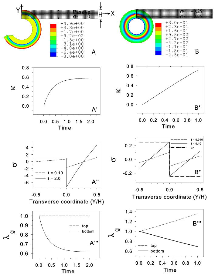
Cantilever beam with stress feedback. (A–A‴) Bending of beam to growth equilibrium configuration with stress-modulated growth in the bottom layer (target stress = σ* = 1); top layer is passive. (A) Undeformed and deformed configurations. (A′) Beam curvature (κ) increases rapidly at first and then reaches a steady state as the target stress distribution is attained. (A″) Transmural bending stress distribution at two time points. The stress in the bottom layer (−0.5 < Y/H < 0) approaches the target stress (σ* = 1). (A‴) Growth stretch ratio (λg) vs. time at top and bottom of beam. In the growing region (bottom), λg decreases and reaches steady state as the target stress is attained. (B–B‴) Perpetual bending of a cantilever beam. Target stresses are specified in the top layer (σ* = −0.25) and bottom layer (σ* = 0.25). (B) Undeformed and deformed configurations. (B′) Beam curvature increases monotonically and does not reach a steady-state. (B″) Transmural stress distribution does reach a steady-state with σ(t) > σ* in the top layer and σ(t) < σ* in the bottom layer for t > 0.01. (B‴) Growth in the top layer and atrophy (contraction) in the bottom layer continue indefinitely. Vertical line in (A) denotes the section used in (A″) and (B″). Black rectangles in (A) indicate the elements at which time plots for λg are generated (A‴,B‴). Colors in (A) and (B) indicate longitudinal Cauchy stress distributions relative to deformed beam geometry.
Figure 4.
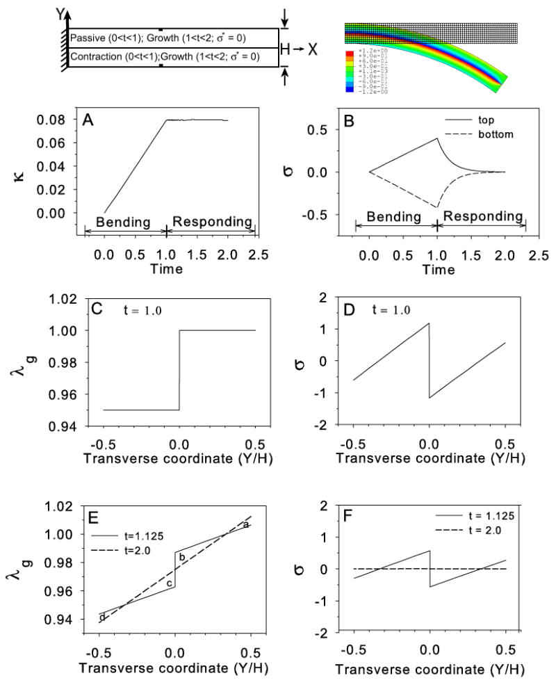
Stress relaxation in a cantilever beam. Top row shows schematic (left) and undeformed and deformed configurations (t ≥ 1.0, right). Bottom layer contracts for 0 ≤ t ≤ 1 (bending phase) and remains at maximum contraction thereafter; both layers grow in response to stress (σ* = 0) for 1 < t ≤ 2 (responding phase). Colors indicate longitudinal Cauchy stress distribution relative to deformed beam geometry. (A) Beam curvature increases steadily during the bending phase and remains unchanged during the responding phase. (B) Bending stresses (at elements indicated by filled rectangles in schematic) increase in magnitude at top and bottom of beam during the bending phase and drop to zero during the responding phase. (C,D) Transmural distributions of λg and σ at start of the responding phase. (E,F) Distributions of λg and σ at t = 1.125 (solid line) and at the end of the responding phase (t = 2.0, dashed line). Please see Fig. 3A for section used in C–F.
As discussed by Rodriguez et al. (1994), it is immaterial whether rigid-body rotation is included in K or G. Here, we include it in K and write
| (7) |
Most biological tissues contain at least orthotropic symmetry. In this case, if growth occurs only along principal material directions, we can ignore shearing relative to these directions due to growth and take the special form
| (8) |
In this expression, the λgi are growth stretch ratios along the local directions Ei, which correspond to principal material directions in the initial stress-free state (B0 in Fig. 2). We now need to find the appropriate components of K to use in the constitutive law of Eq. (2).
Substituting Eq. (7) into Eq. (1) and extracting the components of F defined by Eq. (3) yields
| (9) |
In these relations, δij = Ei ⋅ Ej = ei ⋅ ej is the Kronecker delta, and the last line is given by Eq. (6). In matrix form, Eq. (9) can be written
| (10) |
where the matrices are populated by the components defined by Eqs. (3), (6), and (7). Thus, if the Gij and Rij are known, and with the Fij passed into UMAT, the elastic deformation gradient components are given by
| (11) |
This matrix equation provides the appropriate components of K to be used in UMAT.
2.3 Material Properties
Relatively few data are available for the mechanical properties of embryonic tissues (Forgacs et al., 1998; Davidson et al., 1999; Zamir et al., 2003; Zamir and Taber, 2004). Some measurements indicate that embryonic tissues are more linear than mature tissues, and some investigators have suggested that embryonic epithelia behave as a viscous fluid during the slow process of morphogenesis (Forgacs et al., 1998; Beysens et al., 2000). Embryonic tissues contain residual stress, however, indicating that elasticity cannot be neglected and that stress-induced deformation is limited (Taber et al., 1993; Beloussov, 1998; Zamir and Taber, 2004). For simplicity, we herein ignore viscous effects and consider a mechanically isotropic material characterized by a modified neo-Hookean strain-energy density function of the form
| (12) |
where Ī = J−2/3tr K = J−2/3(3+2εii) and J = det K = [det(δij +2εij)]1/2 are strain invariants, and C and D are material constants. For a nearly incompressible material, J → 1 and D → 0. Because qualitative behavior is the focus of this paper, neglecting viscoelasticity should not significantly affect the main conclusions. In addition, all quantities are taken in a nondimensional form, and we take C = 10 and D = 0.1.
Cytoskeletal contraction is an important generator of morphogenetic force. Contraction can be simulated by assuming that an isolated contractile fiber stiffens and shortens to a new stress-free configuration, analogous to negative growth. This method for modeling contraction is analogous to the time-varying elastance concept in cardiac mechanics (Taber and Perucchio, 2000). In this paper, we simulate contraction by taking λg1 < 1 along the fiber direction E1. For simplicity, however, the stiffness (depending on the value of C) remains unchanged unless stated otherwise.
2.4 Growth Law
In the embryo, tissues alter their dimensions in several ways, including growth and contraction. In this paper, we use the term “growth” to indicate an active adaptation in response to a specified target stress. The response can include actual tissue growth as well as contraction.
The stress state of a specimen is altered due to growth. Conversely, growth is influenced by the stress state, leading to a closed-loop feedback system. In this paper, we explore a growth law of the form
| (13) |
where DG is the growth rate tensor,
 is a fourth-order tensor of growth coefficients, σ is the Cauchy stress tensor, and σ* is the target stress, i.e., the stress at growth equilibrium. The present analysis is based on tensor components defined by the representations DG = (DG)ijEiEj,
= AijklEiEjekel, σ = σijeiej, and
.
is a fourth-order tensor of growth coefficients, σ is the Cauchy stress tensor, and σ* is the target stress, i.e., the stress at growth equilibrium. The present analysis is based on tensor components defined by the representations DG = (DG)ijEiEj,
= AijklEiEjekel, σ = σijeiej, and
.
For simplicity, all of the beam and cylinder models in this paper consider growth (or contraction) in (say) the E1 direction only. Then, with
= aE1E1e1e1, Eq. (13) yields the one-dimensional growth law
| (14) |
where the constant a characterizes the rate of growth and σ is the normal stress in the rotated e1 direction. More specifically, growth occurs in the longitudinal (X) direction for beams and in the circumferential direction for cylinders. For spherical shells, equal growth is assumed to occur in the circumferential and meridional directions. Note that the quantity DG represents the rate of growth per unit length in the zero-stress state B (Fig. 2), whereas λ̇g is the growth rate per unit reference length in state B0. In this paper, a = 1 unless stated otherwise.
It is important to mention that, in our models, growth is anisotropic, although the material is taken as initially isotropic. This potential biological inconsistency should not influence the overall qualitative behavior of our models.
Within UMAT, Eq. (14) is discretized as
| (15) |
where Δt is the integration time step. In this qualitative study, time is an arbitrary parameter and Δt is chosen such that the total time of simulation is divided into at least 400 increments. Note that Eq. (14) is the mathematical representation of the feedback system shown in Fig. 1.
2.5 Finite Element Details
All simulations were run in ABAQUS Version 6.4. In addition to the Cauchy stress tensor, UMAT also requires coding for the fourth-order spatial tensor of elasticities
 ,1 which contains the derivative of each stress component with respect to each strain component. The procedure for computing
is described in Appendix B.
,1 which contains the derivative of each stress component with respect to each strain component. The procedure for computing
is described in Appendix B.
Plane strain analysis was used for problems involving beams (actually “plates”) and cylinders, while spherical shells were analyzed using axisymmetry. Second-order quadrilateral elements were used for the beam problems (mesh is shown in Fig. 3A,B). Fixed time-step analysis was used with Δt = 0.001 (invagination problems) and Δt = 0.005 (beam-bending problems) and any delay in the feedback loop was selected such that the delay time, d, is always a multiple of the simulation step time [please see Eq. (16) below]. This ensures that the delayed system state at time t − d always coincides with a formerly iterated equilibrium state and no interpolation is necessary.
The growth law in Eq. (15) was implemented using solution-dependent state variables within subroutine UMAT. These state variables allow storage of any variable at any time instant during simulation. This list includes all stress and strain components, as well as any other variables (such as λg) that are defined by the user. Within UMAT, the stored value can then be used in future time instants, where its value can be optionally updated or simply left alone. It is important to note that state variables are fields, just like stress and strain, which means that at every time instant, there is a unique value for every integration point. Additionally, state variables are available to the output database, so that their time history or field distribution can be plotted.
This feature was used to update λg at each time step according to Eq. (15). To illustrate how a time delay was included, consider, for example, the case where d = 3Δt. Initially, the stress at t = 0Δt, t = 1Δt, and t = 2Δt are stored in three separate state variables var1, var2, and var3, respectively. At t = 3Δt, the value of the delayed stress, σ(t − 3Δt) = σ(0), is directly read from var1. At t = 4Δt, the value of the delayed stress, σ(t – 3Δt) = σ(1Δt), is directly read from var2, and so on.
For fluid-filled shells, the cavity was lined with hydrostatic incompressible fluid elements, which maintain a constant cavity volume and provide a hydrostatic pressure through a Lagrange multiplier. The fluid constitutive model is available as a standard tool in ABAQUS and, for the large deformation problems considered in this paper, the introduction of the Lagrange multiplier did not introduce any numerical instabilities. In addition, it was verified that the cavity volume did not change during simulation. Since the current version of ABAQUS supports only linear fluid elements, the shell simulations are based on a compatible linear mesh; a very dense mesh (13,000 elements) was used in these problems to maintain accuracy.
Note that growth can be implemented in other commercial codes that allow access to constitutive relations and the components of the deformation gradient tensor. In fact, as mentioned earlier, several of the models discussed in this paper were also solved using COMSOL Multiphysics, and the results were found to be identical.
3 Results
To illustrate the value of ABAQUS in studying morphogenesis, we herein consider some representative bending problems. Bending of epithelia is central to a number of developmental processes, including gastrulation (Davidson et al., 1995), neurulation (Clausi and Brodland, 1993), and cardiogenesis (Taber, 2005). The emphasis here is on the possible role of mechanical feedback. First, to fix ideas, we examine bending of a beam composed of two layers, which can represent a two-cell-thick epithelium, e.g., germ layers in an embryo or an epithelium with attached basal lamina. Then, we extend the analysis to study invagination in circular tubes and spheres, with and without an enclosed fluid.
Our basic premise is that genes signal a regional change in target stress σ*, which stimulates a growth response that alters the stress field. The tissue then responds by growing or contracting2 in an attempt to return stresses toward their homeostatic values. For simplicity, external loads other than cavity pressure are ignored, and all simulations begin with a zero-stress configuration (with zero pressure); hence, the tissue is in a homeostatic condition as long as the target stress remains uniformly zero.
3.1 Stress feedback in a cantilever beam
As in a heated bimetallic strip, differences in growth or contraction between layers cause a beam to bend. Here, we consider two problems. In the first problem, an axial growth law [Eq. (14)] is specified in the bottom layer with a target stress . The top layer is passive (Fig. 3A). In response to the change in σ*, negative axial growth (or contraction) occurs in the lower layer (Fig. 3A‴), causing tension that bends the beam downward.3 Bending ceases when σ* = 1 throughout the lower layer (Fig. 3A′,A″). Note that the stress distribution in the top layer (0 ≤ Y/H ≤ 0.5) changes dramatically to satisfy equilibrium (Fig. 3A″), as the net axial force and bending moment must be zero at all times. (The local end effects apparent in the deformed beams of Fig. 3A,B should not influence the gross behavior.)
In the second problem, both layers actively respond to perturbations in target stresses, with σ* = 0.25 specified in the low layer and σ* = −0.25 in the upper layer (Fig. 3B). Because this stress distribution satisfies force but not moment equilibrium, the beam bends perpetually as it chases these target stresses (Fig. 3B′). Interestingly, the bending stress distribution does not change appreciably as the beam bends and soon reaches a steady state (Fig. 3B″). Since the steady-state stress distribution (Fig. 3B″, solid line) does not match the target stress distribution (dash-dot line), the growth stretch ratios continue to increase in magnitude (Fig. 3B‴), leading to perpetual bending (Fig. 3B′).4
3.2 Stress relaxation in a cantilever beam
As mentioned above, some researchers have postulated that embryonic tissues behave as viscous fluids (Forgacs et al., 1998; Beysens et al., 2000). In this case, morphogenetic shape changes would occur without generating sustained residual stress, i.e., σ* = 0. The following example illustrates some consequences of this assumption for a bilayered cantilever beam. The simulation consists of two phases:
Bending phase (0 ≤ t ≤ 1): Axial contraction (negative growth) is specified in the lower layer (λg drops from 1.0 to 0.95), while the upper layer remains passive. There is no feedback in this step.
Responding phase (1 < t ≤ 2): An axial growth law [Eq. (14), with a = 0.175] is assigned to both layers with the target stress set at σ* = 0. The initial condition for the contracted layer is λg = 0.95.
The results show that the beam curvature increases monotonically during the bending phase and remains constant thereafter (Fig. 4A). Due to downward bending, axial stresses are tensile at the top and compressive at the bottom of the beam during the bending step, but drop to zero in the responding step. In other words, the beam remains bent at the curvature caused by the initial contraction while the bending stress approaches zero (the target stress) throughout the beam (Fig. 4B). This behavior is explained as follows.
Consider the changing growth and bending stress distributions in the beam (Fig. 4C–F). At the end of the bending phase (t = 1), both λg and σ are discontinuous between layers. During the responding phase, according to the growth law of Eq. (14), growth occurs in regions of tension to reduce the stress, while contraction occurs in regions of compression to increase stress. This response gradually reduces the stress to zero throughout the beam (Fig. 4F), as the distribution of λg becomes continuous and linear (Fig. 4E). Surprisingly, the curvature does not change during this phase because increases and decreases in λg across the beam effectively cancel out. In Fig. 4E, for instance, area a = area d and area b = area c.
3.3 Cantilever beam oscillations
According to classical control theory, a feedback control system with a delay in the feedback loop can lead to oscillations in the controlled variable. Depending on the delay magnitude, oscillations may be damped, sustained, or unbounded (Franklin et al., 1997). Because it is likely that biological systems do not respond instantly to perturbed loading conditions, we consider a simple morphogenetic model that includes a time delay.
The simulation in the previous section is repeated with the modified axial growth law
| (16) |
where the delay time d is taken as an integer multiple of the integration time step Δt = 0.005. During the responding phase, both σ and λg oscillate. Our choice of delay (d = 0.030, about one-fourth the oscillation period) leads to damped oscillations (Fig. 5A′). Increasing the delay magnitude can lead to sustained oscillations or unstable behavior (results not shown). As in the previous example, the symmetry in the problem ensures that changes in λg in the upper and lower layers of the beam effectively cancel out (Fig. 5A″, area a = area d and area b = area c), and hence the beam itself does not oscillate (Fig. 5A).
Figure 5.

Cantilever beam oscillations. Bottom layer contracts for 0 ≤ t ≤ 1 (bending phase) and remains at maximum contraction thereafter; both layers grow in response to stress (σ* = 0) with a time delay for 1 < t ≤ 2 (responding phase). (This model is the same as that of Fig. 4 except for the delayed response.) (A)–(A″) Materially homogeneous beam; stress oscillations occur without bending oscillations. (B)–(B″) Materially inhomogeneous beam (modulus of top layer > modulus of bottom layer); both stress and bending oscillations occur. (A,B) Beam curvature vs. time. (A′,B′) Bending stress vs. time at element indicated by filled rectangle in schematic. (A″,B″) Change in transmural distribution of λg during a small representative time interval (from t = 1.00 to t = 1.02). For the beam on the left, the increases and decreases in λg cancel out (area a = area d and area b = area c); hence the curvature does not oscillate. For the beam on the right, the transmural change in λg from t = 1.0 to t = 1.02 is not symmetric (B″:area a ≠ area d and area b ≠ area c), leading to bending oscillations. See text for details. Please see Fig. 3A for section used in A″,B″.
This symmetry can be broken by increasing the modulus of the top layer of the beam relative to the bottom layer. Accordingly, the ratio of moduli S = Ctop/Cbottom was increased from 1 to 3. In addition, the delay magnitude was decreased to d = 0.015 to get sustained oscillations (see note below). This leads to stress oscillations as before (Fig. 5B′), but the transmural change in λg is no longer symmetric (Fig. 5B″, area a ≠ area d and area b ≠ area c), and the beam starts to oscillate (Fig. 5B).
Here, it is important to note the following. The stress-only oscillation (Fig. 5A-A″) and beam oscillation (Fig. 5B–B″) simulations use slightly different time delays. For d = 0.030, the beam oscillation problem was found to be highly sensitive to the value of S. For example, S = 1.3 leads to large unstable oscillations, while S = 1.25 does not produce any oscillations. On the other hand, d = 0.015 did not cause any stress fluctuations in the stress oscillation problem and results were identical to those in Fig. 4, where d = 0. Overall, it was found that a large enough delay in the feedback law is sufficient to introduce stress oscillations without beam oscillations and that both a delay and S > 1 are needed for stress oscillations that are accompanied by beam oscillations. Note that the time period, T, of the induced oscillations is also different in the two cases (Fig. 5A′,B′) but T/d ≈ 4.4 in both cases. Note also that bending oscillations are also produced for S < 1 (results not shown). Bending oscillations occur whenever the elastic moduli of the two layers differ.
3.4 Invagination
Invagination, the local infolding of a region of epithelial cells, plays a vital role in various morphogenetic processes during embryogenesis. During neurulation, for example, a furrow forms and closes off to create the neural tube, while sea urchin gastrulation involves the dimpling of a fluid-filled ball of cells called the blastula (Gilbert, 2006). Here, we illustrate how simple feedback laws drive invagination in cylindrical and spherical shells (Fig. 6), which approximate the geometry for a number of early embryos.
Figure 6.

Invagination in a cylindrical shell (A–C) and spherical shell (A′–C′). Undeformed (dotted) and deformed (solid) configurations are shown for empty shells (A,A′) and fluid-filled shells (B,B′). Coordinate directions are as indicated. Target stresses indicated in (A) apply to all cases: shaded region denotes contracting region (σ* = 6; active modulus = 2 × passive modulus); region immediately above active region is passive; growth with σ* = 0 everywhere else. For the spherical shell, the same values of σ* are specified in both the circumferential (θ) and meridional (ϕ) directions. (C,C′) Fluid pressure vs. time for above fluid-filled shells.
The deformation is assumed to be plane strain for the cylinders and axisymmetric for the spheres. The regional material properties and growth laws are effectively the same for all cases. Contraction is specified through the growth law (σ* = 6 with active modulus = 2 × passive modulus) in a small region of the outer wall (Fig. 6A). The wall is passive inward from the contracted region, and the remainder of the wall grows with σ* = 0. For the cylinder, growth and contraction occur only in the circumferential direction (θ); for the sphere, growth and contraction are equal in the meridional (ϕ) and circumferential (θ) directions (see Fig. 6A,A′). Results are shown for shells with and without an enclosed incompressible fluid, which keeps the cavity volume constant for all time.
The contraction induces a local inward bending. In the absence of internal fluid, the amount of invagination in the cylindrical shell is much greater than in the spherical shell (Fig. 6A,A′). This difference is caused by circumferential (hoop) stress, which effectively stiffens the spherical shell.
The introduction of internal fluid dramatically reduces the amount of invagination in the cylindrical shell (Fig. 6A,B), while there is only a marginal decrease in the spherical shell (Fig. 6A′,B′). In the fluid-filled shell, deformation is resisted by stretching of the shell elsewhere, which requires significantly more force than bending and limits the amount of fluid that can be displaced by the invaginating cells. The differences between the deformed fluid-filled shells also are significant, although less dramatic (Fig. 6B,B′). Note that the building fluid pressure closes the tube that forms at the apex of the cylindrical shell (Fig. 6B), while the spherical invagination remains open (Fig. 6B′).
Fluid pressure vs. time plots are shown for the two fluid-filled shells (Fig. 6C,C′). For both shells, the onset of invagination coincides with a sharp rise in pressure, as the displaced fluid stretches the shell outside the dimple. The pressure then drops as the shell grows in response to pressure-induced wall tension. The peak pressure in the spherical shell is smaller and decays faster than that of the cylindrical shell.
3.5 Elastic snap-through
Elastic snap-through is sometimes observed during morphogenesis. Examples include inversion in volvox embryos (Viamontes and Kirk, 1977; Viamontes et al., 1979) and archenteron formation during gastrulation in the sea urchin (Davidson et al., 1995). Figure 7 illustrates how increased stiffness of the active region can lead to snap-through (buckling) in a spherical shell. Compared to Fig. 6B, the active region (σ* = 25) is expanded slightly and the active modulus is increased to 10 times the passive modulus (Fig. 7A). This leads to dramatic jump in deformation during invagination, accounting for more than 60% of the total amount of invagination (Fig. 7B,C). During snap-through, the transition from one geometry to another (insert in Fig. 7A) is essentially instantaneous.
Figure 7.

Elastic snap-through during invagination in a spherical shell (no fluid). (A) Undeformed (dotted) and deformed (solid) configurations. Shaded region denotes active region (σ* = 25.0; active modulus = 10 × passive modulus); region immediately above the active region is passive; growth with σ* = 0 everywhere else. Target stresses are specified in both the meridional and circumferential directions. Insert shows the configurations immediately before (t = 0.009) and after (t = 0.01) snap through. (B) Vertical displacement vs. time at node T (indicated in A). (C) Vertical displacement vs. λg at node T (indicated in A). Arrows in (B) and (C) denote the sudden increase in displacement due to snap through.
4 Discussion
Interest in morphomechanics has intensified in recent years, as increasing numbers of researchers have come to appreciate the crucial role that mechanics plays in the development of tissues and organs. In designing strategies for tissue engineering, both the chemical and mechanical environment must be considered. Computational modeling can be a valuable tool in this process.
Although it is generally accepted that development involves mechanical forces, how these forces are regulated remains a subject for debate. Some researchers believe that active force generation merely follows the instructions of genes and chemical prepatterns. On the other hand, there is growing evidence that mechanical feedback plays a prominent role in force regulation (Beloussov, 1998). According to the hyper-restoration (HR) hypothesis of Beloussov (1998), a perturbation in tissue stress induces an active mechanical response that is directed toward restoring the initial stress value (target stress), but generally overshoots to the opposite side. Each response changes tissue shape and induces a new stress perturbation, which elicits a new response, and so on, until the proper form is created. Beloussov has shown that this idea can explain in qualitative terms a number of experimental observations for embryos undergoing various morphogenetic events, including cleavage, gastrulation, and neurulation (Beloussov, 1998).
Here, we have assumed that the target stress is controlled by biology, e.g., the genes. This is a very simple concept, but our simulations have shown that it can lead to complex morphogenetic behavior. It is possible that genetic and molecular signals control the value of σ* at all points in space and time, but this is not likely or necessary. Changing the target stress in one small region induces deformation that changes the stress field in nearby regions, which then respond to this perturbation, and so on. This is the essence of Beloussov's hypothesis.
There is debate as to whether embryonic tissues are viscoelastic solids or viscoelastic fluids. Clearly, embryos exhibit fluid-like behavior, as they do not return to their original configuration when external loads are removed. Moreover, morphogenesis often involves the spreading of one cell layer over another or the sorting of different cell types, behavior similar to that of a mixture of immiscible liquids (Forgacs et al., 1998; Beysens et al., 2000; Brodland and Chen, 2000; Brodland, 2002). As already noted, however, most embryonic tissues contain residual stress (Beloussov et al., 1975; Taber et al., 1993; Beloussov, 1998; Zamir and Taber, 2004), which a viscoelastic fluid cannot sustain over large time scales. This suggests solid-like behavior. The plasticity observed in developing embryos is likely due to growth and remodeling rather than liquid-like viscoelastic or plastic flow. The models presented in this paper illustrate this point, as they change shape permanently without externally applied loads.
It is important to note that the models presented here are only for illustration; we have not attempted to develop a model specific to any particular organism. We expect that including realistic material properties, for example, would affect the behavior quantitatively, but the results likely would be similar qualitatively.
4.1 Relation to Previous Models for Morphogenesis
In the embryo, cells move either individually (mesenchyme) or in sheets (epithelia). Mathematical models have been proposed for both epithelial and mesenchymal morphogenesis.
A pioneering model for mesenchymal morphogenesis is the Murray-Oster model, which is based on continuum mechanics for a mixture of cells and matrix and includes the effects of cell traction (via contraction), cell multiplication, matrix secretion, cell migration, and differential adhesion (Oster et al., 1983; Murray and Oster, 1984). The governing equations produce a reaction-diffusion type system similar to those studied extensively in biochemical models of pattern formation (Murray, 1993). Using this theory, Manoussaki et al. (1996) and Namy et al. (2004) studied two-dimensional models for vasculogenesis, while Barocas and Tranquillo (1997) extended the theory to model the development of cell-populated collagen gels.
Models for epithelial morphogenesis have been used to study cell rearrangement, pattern formation, and invagination (Taber, 1995). The classic paper of Odell et al. (1981) presents an FE model for a blastula consisting of a circular ring of cells. Each cell is represented by a viscoelastic truss-like element, with morphogenesis driven by stretch-activated contraction of apical microfilaments.5 For appropriate choices of model parameters, they obtained deformed shapes consistent with gastrulation, ventral furrow formation, and neurulation. In some models, they enforced a constant cavity volume constraint, as in the models of of Fig. 6B,B′.
In a recent paper, Munoz et al. (2006) investigated invagination with a similar FE model consisting of a cylindrical ring. Their analysis is based on continuum mechanics and a decomposition of the deformation gradient tensor like that in Eq. (1). However, whereas we include only growth without shearing of the unstressed element, they include angle changes in G to allow the stress-free element to take the shape of a trapezoid (when the cell apex contracts), similar to the elements of Odell et al. (1981).6 Their simulations include the effects of constant cavity volume, as well as a constrained outer radius due to the presence of the vitelline membrane in the Drosophila embryo.
A cell ring is a reasonable model for furrow formation and neurulation. However, our results show that including spherical geometry is crucial to modeling the dimpling that occurs during sea urchin gastrulation (Fig. 6A′,B′). Hoop stress makes invagination a much more difficult task, possibly explaining the need for secondary mechanisms, including convergent extension and bottle cells, to help draw the invaginating region (archenteron) to the opposite side of the embryo (Keller, 2003; Gilbert, 2006).
Taking spherical geometry into account, Davidson et al. (1995) studied the initial phase of sea urchin gastrulation using an FE model based on the commercial code NASTRANS. Their model is similar to our spherical model without fluid (Fig. 6A′), except the material properties were taken as linear. Also similar to our work, they used isotropic volumetric expansion and shrinkage to simulate swelling and contraction, respectively. Using this model, they investigated several possible mechanisms for invagination.
In other related work, Belintsev et al. (1987), Taber (2000), and Taber and Zahalak (2001) used continuum models for epithelia to study pattern formation. In addition, extending an idea presented by Weliky and Oster (1990), Brodland and colleagues have developed cell-level models for epithelial morphogenesis (Brodland and Clausi, 1994; Brodland and Chen, 2000; Chen and Brodland, 2000; Brodland, 2002). With adhesive, microfilament, membrane, and other cytoskeletal forces lumped into a single equivalent tension at cell boundaries, these authors have obtained impressive results for neurulation and cell sorting. Our present models do not account for details at the cell level.
Finally, Ramasubramanian et al. (2006) have presented a three-dimensional FE model for early heart development (looping) that was developed in ABAQUS using the techniques introduced here. This model includes simultaneous application of various morphogenetic processes such as growth, cytoskeletal contraction, and active cell-shape changes.
4.2 Development Regulated by Mechanical Feedback
In most of the models discussed above, morphogenetic forces are prescribed. A notable exception is the model of Odell et al. (1981), who assume that cells are stretch activated, i.e., they contract when deformed beyond a critical value of stretch. In all of the models included in this paper, growth and contraction are assumed to be modulated by the local stress state. For simplicity, we have assumed that the rate of growth depends linearly on the difference between the current stress and a homeostatic stress [see Fig. 1 and Eq. (14)]. This form of growth law is consistent with experimental data from cardiovascular mechanics (Taber, 2001), as well as with Beloussov's HR hypothesis. Consider, for example, uniaxial deformation of a bar. If the bar is stretched and held at a fixed length (σ > σ*), it grows to return the stress to σ*. However, if the bar is shortened and held (σ < σ*), it contracts to generate a tension that returns the stress to σ*.7 With the value of σ* specified, presumably by genes, our results show that the simple growth law in Eq. (14) can lead to a wide array of morphogenetic behaviors including controlled bending (Fig. 3A′–A‴), perpetual bending (Fig. 3B′–B‴), stress relaxation (Fig. 4), stress and strain oscillations (Fig. 5), invagination (Fig. 6), and elastic snap-through (Fig. 7).
Genetic control of target stress, however, raises the following question: How do the genes know that the specified stress field satisfies equilibrium? It is not likely that genes draw free-body diagrams to determine their next move. Consider, for example, the beam bending problems in Fig. 3. Non-equilibrating target stresses are specified throughout the beam in panel B, and the beam bends continually. However, the problem in panel A offers a possible answer to the posed question. Here, part of the beam remains passive, allowing this region to adjust its stresses as equilibrium demands (Fig. 3A″). The beam bends until the active region reaches the specified target stress, and then bending stops. Hence, the presence of a passive region precludes unbounded changes in form. We speculate that the basal lamina may furnish such a passive layer for an epithelium.
4.3 Modeling of Morphogenetic Processes
With certain limitations, the growth theory of Rodriguez et al. (1994) can be used to simulate a number of mechanisms that are fundamental to both mesenchymal and epithelial morphogenesis. We already have shown how cytoskeletal contraction can be simulated. Active cell-shape change caused by elongating microtubules or growing actin filaments can modeled similarly by taking λgi > 1 along the expanding directions with a constant cell volume constraint enforced in the other directions (λg1λg2λg3 = 1). Cell migration can be simulated by atrophy in one region and equal growth in another region. However, these are relatively crude macroscopic representations of what are certainly complex processes at the cell level. More detailed modeling of these mechanisms could be done using multiscale techniques (Agoram and Barocas, 2001).
4.4 Commercial Codes vs. Custom Codes
For some problems in morphogenesis, the best (and maybe only) option is to develop a customized FE program. A good example is the cell-level model used by Brodland and co-workers to study cell sorting (Brodland, 2002). Custom codes, however, can take years to develop, with significant investment in program development in addition to problem solving. If phenomenological modeling is adequate, many morphomechanical problems can be solved by proper use and modification of commercial FE codes.
For example, many of the problems in this paper can also be done using COMSOL Multiphysics. In general, we have found that ABAQUS is very good in dealing with 3D problems. On the other hand, COMSOL provides access to the governing equations, making it generally more flexible than ABAQUS. Currently, however, COMSOL does not handle 3D problems as well as ABAQUS.
In this paper, we have shown how ABAQUS can be extended in a relatively straightforward manner to handle a variety of problems in morphogenesis involving growth and contraction. The availability of computational tools such as this should aid efforts to understand the role of mechanics in tissue and organ development.
Acknowledgments
The authors wish to thank professor Barna Szabo for his helpful comments on improving the accuracy of the finite element models. This work was supported by grants F32 HL79764 (AR) and R01 HL64347, R01 GM075200, and R01 HL083393 (LAT) from the National Institutes of Health.
Appendix A: Computation of Rotation Tensor
The rotation tensor R is computed as follows. First, the components of the total deformation gradient tensor, F, which are passed into UMAT are used to compute the left Cauchy-Green deformation tensor, B = F·FT. Next, the SPRIND subroutine is called to provide the eigenvalues (λni, the principal stretch ratios) and the eigenvectors (ni, the orthogonal principal directions in the deformed configuration) of B. The left stretch tensor, is then given by (Taber, 2004)
| (A1) |
and Eq. (5) yields R = V−1 · F. Note that the total deformation gradient tensor is used to compute R.
Appendix B: Computation of the Spatial Tensor of Elasticities
In ABAQUS/UMAT, the spatial tensor of elasticities
is defined through the relation
| (B1) |
where D is the rate-of-deformation tensor, and τ˚ = τ˙ − Ω · τ + τ · Ω is the Jaumann rate of the Kirchoff stress τ = Jσ, with Ω being the spin tensor. For a general orthotropic strain energy-density function, the components of
are provided in Eq. (11.9) of Lubarda and Hoger (2002). For an isotropic material, a simplified expression is given in Eq. (6.193) of Holzapfel (2001). These components are computed in UMAT.
Appendix C: Computation of Beam Curvature
The amount of bending for simulations involving cantilever beams is quantified by the beam curvature. Let (X, Y) and (x, y) be the Cartesian coordinates of a point near the center of the beam before and after deformation, respectively. The nondimensional curvature is given by (Yang and Feng, 1970)
| (C1) |
where
| (C2) |
In these expressions, prime denotes differentiation with respect to X, and H is the undeformed beam thickness. To avoid end effects, the curvature was computed near the middle of the beam.
Footnotes
The tensor
is referred to as the “Jacobian matrix” and “consistent Jacobian” in the ABAQUS manuals. It is also referred to as the “spatial tensor of elasticities” in Holzapfel (2001) and as the “elastic moduli tensor” in Lubarda and Hoger (2002). In addition, it is referred to as the “continuum tangent operator” in the inelasticity literature. Here, we use the terminology of Holzapfel (2001).
Programmed cell death (apoptosis) is an important mechanism in embryogenesis. In general, however, epithelia alter their form by contracting, growing through cell multiplication, or changing shape by cell intercalation. In this paper, we refer to any negative growth as “contraction.”
In all beam problems, curvature was computed near the center of the beam as described in Appendix C.
Eventually, the beam bends all the way around and starts to self-intersect, as no contact conditions are specified in this simulation. This, however, is unrealistic unless we consider bending that continues in a different plane.
It is interesting to note that Odell et al. (1981) modeled active contraction through a change in zero-stress length, similar to the method used here.
In the present work, apical contraction is simulated by representing the contracting apex and the rest of the cell by separate element layers.
In this paper, we ignore any overshoot of the target stress when the tissue responds to stress perturbations.
References
- ABAQUS/Standard User's Manual. I and III. ABAQUS, Inc. Providence; Rhode Island: 2003. [Google Scholar]
- Agoram B, Barocas VH. Coupled macroscopic and microscopic scale modeling of fibrillar tissues and tissue equivalents. Journal of Biomechanical Engineering. 2001;123:362–369. doi: 10.1115/1.1385843. [DOI] [PubMed] [Google Scholar]
- Barocas VH, Tranquillo RT. An anisotropic biphasic theory of tissue-equivalent mechanics: the interplay among cell traction, fibrillar network deformation, fibril alignment, and cell contact guidance. Journal of Biomechanical Engineering. 1997;119:137–145. doi: 10.1115/1.2796072. [DOI] [PubMed] [Google Scholar]
- Belintsev BN, Beloussov LV, Zaraisky AG. Model of pattern formation in epithelial morphogenesis. Journal of Theoretical Biology. 1987;129:369–394. doi: 10.1016/s0022-5193(87)80019-x. [DOI] [PubMed] [Google Scholar]
- Beloussov LV, Dorfman JG, Cherdantzev VG. Mechanical stresses and morphological patterns in amphibian embryos. Journal of Embryology and Experimental Morphology. 1975;34:559–574. [PubMed] [Google Scholar]
- Beloussov LV. The Dynamic Architecture of a Developing Organism: An Interdisciplinary Approach to the Development of Organisms. Kluwer, Dordrecht; The Netherlands: 1998. [Google Scholar]
- Beysens DA, Forgacs G, Glazier JA. Cell sorting is analogous to phase ordering in fluids. Proceedings of the National Academy of Sciences. 2000;97:9467–9471. doi: 10.1073/pnas.97.17.9467. [DOI] [PMC free article] [PubMed] [Google Scholar]
- Brodland GW. The differential interfacial tension hypothesis (DITH): A comprehensive theory for the self-rearrangement of embryonic cells and tissues. Journal of Biomechanical Engineering. 2002;124:188–197. doi: 10.1115/1.1449491. [DOI] [PubMed] [Google Scholar]
- Brodland GW, Chen HH. The mechanics of heterotypic cell aggregates: Insights from computer simulations. Journal of Biomechanical Engineering. 2000;122:402–407. doi: 10.1115/1.1288205. [DOI] [PubMed] [Google Scholar]
- Brodland GW, Clausi DA. Embryonic tissue morphogenesis modeled by FEM. Journal of Biomechanical Engineering. 1994;116:164–155. doi: 10.1115/1.2895713. [DOI] [PubMed] [Google Scholar]
- Chen HH, Brodland GW. Cell-level finite element studies of viscous cells in planar aggregates. Journal of Biomechanical Engineering. 2000;122:394–401. doi: 10.1115/1.1286563. [DOI] [PubMed] [Google Scholar]
- Clausi DA, Brodland GW. Mechanical evaluation of theories of neurulation using computer simulations. Development. 1993;118:1013–1023. [Google Scholar]
- Davidson LA, Koehl MAR, Keller R, Oster GF. How do sea urchins invaginate? Using biomechanics to distinguish between mechanisms of primary invagination. Development. 1995;121:2005–2018. doi: 10.1242/dev.121.7.2005. [DOI] [PubMed] [Google Scholar]
- Davidson LA, Oster GF, Keller RE, Koehl MAR. Measurements of mechanical properties of the blastula wall reveal which hypothesized mechanisms of primary invagination are physically plausible in the sea urchin stronglylocentrotus purpuratus. Developmental Biology. 1999;209:221–238. doi: 10.1006/dbio.1999.9249. [DOI] [PubMed] [Google Scholar]
- Davies JA. Mechanics of Morphogenesis. Elsevier Academic Press; New York, New York: 2005. [Google Scholar]
- Forgacs G, Foty RA, Shafrir Y, Steinberg MS. Viscoelastic properties of living embryonic tissues: a quantitative study. Biophysical Journal. 1998;74:2227–2234. doi: 10.1016/S0006-3495(98)77932-9. [DOI] [PMC free article] [PubMed] [Google Scholar]
- Franklin GF, Powell JD, Workman ML. Digital control of dynamic systems. 3rd. Addison Wesley Longman; Menlo Park, California: 1997. [Google Scholar]
- Gilbert SF. Developmental Biology. 8th. Sinauer Associates; Sunderland, Massachusetts: 2006. [Google Scholar]
- Gordon R. Mechanics in embryogenesis and embryonics: prime mover or epiphenomenon ? International Journal of Developmental Biology. 2006;50:245–253. doi: 10.1387/ijdb.052103rg. [DOI] [PubMed] [Google Scholar]
- Holzapfel GA. Nonlinear Solid Mechanics: A Continuum Approach for Engineering. John Wiley and Sons; West Sussex, England: 2001. [Google Scholar]
- Keller R, Davidson LA, Shook DR. How we are shaped: The biomechanics of gastrulation. Differentiation. 2003;71:171–205. doi: 10.1046/j.1432-0436.2003.710301.x. [DOI] [PubMed] [Google Scholar]
- Lubarda VA, Hoger A. On the mechanics of solids with a growing mass. International Journal of Solids and Structures. 2002;39:4627–4664. [Google Scholar]
- Manoussaki D, Lubkin SR, Vernon RB, Murray JD. A mechanical model for the formation of vascular networks in vitro. Acta Biotheoretica. 1996;44:271–282. doi: 10.1007/BF00046533. [DOI] [PubMed] [Google Scholar]
- Munoz JJ, Barrett K, Mindownik M. A deformation gradient decomposition method for the analysis of the mechanics of morphogenesis. Journal of Biomechanics. 2006 doi: 10.1016/j.jbiomech.2006.05.006. In Press. [DOI] [PubMed] [Google Scholar]
- Murray JD. Mathematical Biology. Springer-Verlag; New York, New York: 1993. [Google Scholar]
- Murray JD, Oster GF. Cell traction models for generating pattern and form in morphogenesis. Journal of Mathematical Biology. 1984;19:265–280. doi: 10.1007/BF00277099. [DOI] [PubMed] [Google Scholar]
- Namy P, Ohayon J, Tracqui P. Critical conditions for pattern formation and in vitro tubulogenesis driven by cellular traction fields. Journal of Theoretical Biology. 2004;227:103–120. doi: 10.1016/j.jtbi.2003.10.015. [DOI] [PubMed] [Google Scholar]
- Odell GM, Oster G, Alberch P, Burnside B. The mechanical basis of morphogenesis. I. epithelial folding and investigation. Developmental Biology. 1981;85:446–462. doi: 10.1016/0012-1606(81)90276-1. [DOI] [PubMed] [Google Scholar]
- Oster GF, Murray JD, Harris AK. Mechanical aspects of mesenchymal morphogenesis. Journal of embryology and experimental morphology. 1983;78:83–125. [PubMed] [Google Scholar]
- Ramasubramanian A, Latacha KS, Benjamin JM, Voronov DA, Ravi A, Taber LA. Computational model for early cardiac looping. Annals of Biomedical Engineering. 2006;34:1355–1369. doi: 10.1007/s10439-005-9021-4. [DOI] [PubMed] [Google Scholar]
- Rodriguez EK, Hoger A, McCulloch AD. Stress-dependent finite growth in soft elastic tissues. Journal of Biomechanics. 1994;27:455–467. doi: 10.1016/0021-9290(94)90021-3. [DOI] [PubMed] [Google Scholar]
- Taber LA, Hu N, Pexieder T, Clark EB, Keller BB. Residual strain in the ventricle of the stage 16-24 chick embryo. Circulation Research. 1993;72:455–462. doi: 10.1161/01.res.72.2.455. [DOI] [PubMed] [Google Scholar]
- Taber LA. Biomechanics of growth, remodeling, and morphogenesis. Applied Mechanics Reviews. 1995;48:487–545. [Google Scholar]
- Taber LA. Pattern formation in a nonlinear membrane model for epithelial morphogenesis. Acta Biotheoretica. 2000;48:47–63. [Google Scholar]
- Taber LA. Biomechanics of cardiovascular development. Annual Review of Biomedical Engineering. 2001;3:1–25. doi: 10.1146/annurev.bioeng.3.1.1. [DOI] [PubMed] [Google Scholar]
- Taber LA. Nonlinear Theory of Elasticity. World Scientific; Singapore: 2004. [Google Scholar]
- Taber LA. Biophysical mechanisms of cardiac looping. International Journal of Developmental Biology. 2005;50:323–332. doi: 10.1387/ijdb.052045lt. [DOI] [PubMed] [Google Scholar]
- Taber LA, Perucchio R. Modeling heart development. Journal of Elasticity. 2000;61:165–197. [Google Scholar]
- Taber LA, Zahalak GI. Theoretical model for myocardial trabeculation. Developmental Dynamics. 2001;220:226–237. doi: 10.1002/1097-0177(20010301)220:3<226::AID-DVDY1107>3.0.CO;2-R. [DOI] [PubMed] [Google Scholar]
- Viamontes GI, Kirk DL. Cell shape changes and the mechanism of inversion in volvox. Journal of Cell Biology. 1977;75:719–730. doi: 10.1083/jcb.75.3.719. [DOI] [PMC free article] [PubMed] [Google Scholar]
- Viamontes GI, Fochtmann LJ, Kirk DL. Morphogenesis in volvox: analysis of critical variables. Cell. 1979;17:537–550. doi: 10.1016/0092-8674(79)90262-9. [DOI] [PubMed] [Google Scholar]
- Weliky M, Oster G. The mechanical basis of cell rearrangement: I. Epithelial morphogenesis during fundulus epiboly. Development. 1990;109:373–386. doi: 10.1242/dev.109.2.373. [DOI] [PubMed] [Google Scholar]
- Yang WH, Feng WW. On axisymmetrical deformations of nonlinear membranes. Journal of Applied Mechanics. 1970;37:1002–1011. [Google Scholar]
- Zamir EA, Srinivasan V, Perucchio R, Taber LA. Mechanical asymmetry in the embryonic chick heart during looping. Annals of Biomedical Engineering. 2003;31:1327–1336. doi: 10.1114/1.1623487. [DOI] [PubMed] [Google Scholar]
- Zamir EA, Taber LA. Mechanical properties and residual stress in the stage 12 chick heart. Journal of Biomechanical Engineering. 2004;126:823–830. doi: 10.1115/1.1824129. [DOI] [PubMed] [Google Scholar]