T1ρ-Prepared Balanced Gradient Echo for Rapid 3D T1ρ MRI

Abstract

Purpose

To develop a T1ρ-prepared balanced gradient echo (b-GRE) pulse sequence for rapid 3D T1ρ relaxation mapping within the time constraints of a clinical exam (< 10 minutes), examine the effect of acquisition on the measured T1ρ relaxation time and optimize 3D T1ρ pulse sequences for the knee joint and spine.

Materials and Methods

A pulse sequence consisting of inversion recovery prepared, fat saturation, T1ρ-preparation and b-GRE image acquisition was used to obtain 3D volume coverage of the patellofemoral and tibiofemoral cartilage and lower lumbar spine. Multiple T1ρ-weighted images at various contrast times (TSL) were used to construct a T1ρ relaxation map in both phantoms and the knee joint and spine in vivo. The transient signal decay during b-GRE image acquisition was corrected using a kspace filter. The T1ρ-prepared b-GRE sequence was compared to a standard T1ρ-prepared spin echo sequence and pulse sequence parameters were optimized numerically using the Bloch equations.

Results

The b-GRE transient signal decay was found to depend on the initial T1ρ-preparation and the corresponding T1ρ map was altered by variations in the point spread function with TSL. In a two compartment phantom, the steady state response was found to elevate T1ρ from 91.4 ± 6.5 to 293.8 ± 31 and 66.9 ± 3.5 to 661 ± 207 with no change in the goodness-of-fit parameter R². Phase encoding along the longest cartilage dimension and a transient signal decay kspace filter retained T1ρ contrast. Measurement of T1ρ using the T1ρ-prepared b-GRE sequence matches standard T1ρ-prepared spin echo in the medial patellar and lateral patellar cartilage compartments. T1ρ-prepared b-GRE T1ρ was found to have low interscan variability between four separate scans. Mean patellar cartilage T1ρ was elevated compared to femoral and tibial cartilage T1ρ.

Conclusion

The T1ρ-prepared b-GRE acquisition rapidly and reliably accelerates T1ρ quantification of tissues offset partially by a TSL-dependent point spread function.

Introduction

Conventional contrast in magnetic resonance (MR) images derives from the ¹H magnetic relaxation properties of tissues. Variations in longitudinal magnetic relaxation (T1) and transverse magnetic relaxation (T2) distinguish the healthy and pathological states. An unconventional contrast mechanism based on the rotating frame spin-lattice relaxation time T1ρ (1) shows sensitivity to the diseased states of the human breast (2), early acute cerebral ischemia in rats (3,4), knee cartilage degeneration during osteoarthritis (5), posttraumatic cartilage injury (6) and narrowing of lumbar intervertebral discs associated with degenerative disc disease (7,8). In addition, functional T1ρ imaging shows both an augmented BOLD signal (9,10) and improved response to indirectly detected metabolic H₂¹⁷O (11–13).

T1ρ-weighted contrast is produced in vivo by allowing transverse magnetization to relax in the presence of an on-resonance continuous wave (cw) radiofrequency (RF) pulse and is influenced by motional processes with characteristic frequencies proportional to the amplitude of the cw RF pulse (ν₁ = γB₁/2π). Often, the cw RF pulse is termed a spin-locking pulse because magnetization is ‘locked’ along the direction of the rotating RF field and the spin-locking pulse diminishes the effect of chemical shift, static dipole-dipole and other local interactions of magnetic nuclei. The T1ρ relaxation time may be quantified by obtaining multiple T1ρ-weighted images at different spin-lock durations (TSL). Quantifying relaxation times in pathology provides a measure of disease status and its progression potentially independent of inter- and intrascan variability. In practice, T1ρ-weighted contrast is difficult to implement using rapid acquisition techniques because the cw RF pulse is nonselective and long TRs are necessary to restore equilibrium magnetization.

There is a multitude of imaging sequences to achieve T1ρ-weighted contrast. T1ρ-weighting can potentially be used in 2D, 3D and multislice imaging modalities, employing frequency encoding acquisitions using gradient echo variations both spoiled (FLASH, SPGR, T1-FFE) and unspoiled (FISP, GRASS, FFE), with multiple gradient echoes in a single TR (EPI), spin echo variations (SE) or multiple spin echoes in a single TR (FSE). Similarly, there is no restriction on the number of different k-space trajectories (rectilinear, radial or spiral) that may be used for frequency encoding the T1ρ-weighted magnetization. Common to all T1ρ-weighted imaging sequences is the spin-locking pulse cluster, which, when prepended to the various image acquisition clusters, provides T1ρ-weighting to the magnetization. The spin-locking pulse cluster consists of a similarly varied ensemble of modalities: conventional spin-locking uses a single cw RF pulse sandwiched between excitation and storage RF pulses; rotary echoes can alternate the phase of the cw RF pulse halfway during the spin lock to refocus RF field inhomogeneities (14,15); rotary echoes are combined with spin echoes to refocus both RF and B₀ field inhomogeneities (16); the spin locking pulse may be delivered off-resonance to reduce SAR and provide T1ρ_off contrast (17); or, as an alternative to rectangular cw RF pulses, spin-locking can be achieved adiabatically to modulate the intrinsic relaxation rate dynamically (18). In many cases, these techniques are complementary.

Time constraints during an MR clinical examination place certain restrictions on which T1ρ-weighted imaging sequences are available. For example, T1ρ-weighted imaging in a patient presenting chronic knee joint pain requires a pulse sequence with full volume coverage of the articular cartilage of the patella, femoral condyle and tibial plateau. Two previous implementations are superior to others, a T1ρ-prepared 2D multislice FSE (5,19) or a T1ρ-prepared 3D GRE T1ρ-weighted imaging sequence (5,20). Still, both sequences are probably insufficient for a standard clinical examination with either incomplete volume coverage (multislice) or unreasonably long scan times (> 30 min for 3D GRE). A T1ρ prepared, 3D spoiled GRE sequence provides full volume coverage, but magnetization saturation reduces the SNR because of the short TR (~ 100 ms) and T1-weighting must be compensated (5). The 3D GRE T1ρ map can take as long as 35 minutes (TR = 100 ms, 256 phase encodes, 16 slice phase encodes, 5 T1ρ-weighted images).

A rapid, volumetric T1ρ-weighted imaging sequence is necessary for clinical MR studies, especially if T1ρ mapping is a requirement of the clinical examination potentially with multiple views. We introduce here a T1ρ-weighted imaging sequence that combines standard T1ρ-weighted preparation pulse clusters with a balanced-Steady State Free Precession (b-SSFP or FIESTA, b-FFE, TrueFISP). The T1ρ preparation period and the b-GRE sequence inherently conflict since the former gives T1ρ-weighting to the equilibrium magnetization while the latter abolishes any previous weighting during the approach to the steady-state. Here we demonstrate a method for T1ρ-prepared b-GRE, show how b-GRE acquisition alters T1ρ contrast, numerically optimize the sequence given known T1, T2 and T1ρ relaxation times, map the spatial distribution of T1ρ relaxation times in patellar cartilage and extend these techniques to the human spine in vivo. Further, we constructed a filter to compensate for the loss of T1ρ contrast during b-GRE transient signal decay.

Materials and Methods

Pulse Sequence

The pulse sequence used for T1ρ-prepared b-GRE is shown in Figure 1. The basic sequence consists of a preparatory spin locking pulse cluster consisting of an excitation pulse, cw spin locking pulses (total duration TSL) of alternating phase to form a Solomon rotary echo (14) and amplitude ν₁ = 200–1000 Hz, a storage pulse, and finally a crusher gradient (not shown) to destroy residual magnetization in the transverse plane. Following T1ρ-preparation, magnetization is b-GRE prepared with an α/2 pulse (21), a delay TR/2, and any number of dummy α pulses (N_dummy). The prepared magnetization is subsequently phase and frequency encoded for image acquisition using a standard alternating phase b-GRE acquisition. For 3D T1ρ-prepared acquisition schemes, this basic sequence is followed by a T1 relaxation delay period T_DELAY to restore equilibrium magnetization prior to the next T1ρ preparation period and the slice phase encoding gradients are incremented. This basic sequence can be generalized further to include variable flip angle b-GRE RF pulse trains, segmented k-space acquisition or slice encode during the b-GRE train rather than in-plane phase encode to reduce in-plane blurring. For imaging of cartilage, the T1ρ-preparation period is preceded by a slab selective inversion recovery pulse (TI = 1700 ms) to null joint space fluid and a spectrally selective fat saturation pulse and spoiler gradient.

Figure 1.

Pulse sequence for T1ρ-prepared b-GRE. The sequence consists of a T1ρ preparation period of duration TSL, a b-GRE preparation period consisting of α/2 and phase alternating α dummy pulses, the subsequent phase alternating b-GRE readout and T1 relaxation delay to allow magnetization regrowth to equilibrium. Brackets denote loops in the pulse sequence and the number of times the loop is repeated. For example, ‘x N_ky/2’ means that the loop is repeated for the number of k_y phase encodes divided by 2. To achieve the best T1ρ contrast, N_dummy = 0, however, the number of dummy pulses may be increased to compensate for blurring. For the in vivo experiments of the knee, N_dummy = 1 was optimized by visual inspection for T1ρ map accuracy and minimal blurring.

The Effect of b-GRE Acquisition on T1ρ Contrast

The strategy for b-GRE acquisition of T1ρ-prepared magnetization is to acquire the T1ρ-weighted signal before the b-GRE RF pulse train causes the magnetization to enter the steady-state (21,22). This technique was previously used to continuously acquire the recovery of longitudinal magnetization during an inversion recovery experiment. Depending on the required time resolution and the accuracy of the T1ρ measurement both single-shot and segmented acquisitions can be used. This approach relies on acquiring the T1ρ-prepared magnetization during the transient period of the b-GRE signal evolution, where memory of the T1ρ-prepared magnetization is retained. The transient phase of the b-GRE signal can vary between 50–500 pulses and depends on the flip angle α and tissue T1 and T2 relaxation times (23,24). Low α causes the magnetization to approach the steady-state slowly and higher α approaches the steady-state more rapidly. In the extreme case, α = 180° the magnetization decays at a rate 1/T2 to zero, such as in conventional fast spin echo imaging.

Simulations to determine the effect of the b-GRE transient signal on T1ρ contrast were constructed assuming instantaneous rectangular pulses and instantaneous measurement of echo amplitude at TE (MatLab 7.1; Natick, CT). Figure 2 demonstrates the approach to steady state for 3 different b-GRE flip angles α and 5 different T1ρ contrasts (TSL = 10, 20, 30, 40 and 50 ms). The other parameters for the simulation were T1ρ = 40 ms, T1 = 1 s, T2 = 35 ms, TE = 3.7 ms, TR = 7.4 ms, N_RF = 256. Relaxation times were chosen to mimic knee articular cartilage at 1.5 T. After the first α/2 pulse in the b-GRE RF pulse train, the signal is proportional to the T1ρ weighting:

$$\mathrm{M}(0^{+})={\mathrm{M}}_0{\mathrm{e}}^{-\text{TSL}/\mathrm{T}1\rho }\sin (\mathrm{\alpha }/2)$$ [1]

where 0⁺ denotes the time immediately after the first RF pulse. With each additional α pulse the T1ρ-weighted signal monotonically approaches the steady-state magnetization. For b-GRE flip angles α = 40°or 70° this corresponds to monotonic signal decay during the b-GRE train toward the steady-state; however, if the T1ρ-weighted magnetization is initially smaller than the final steady-state magnetization, the signal can monotonically increase to the steady-state signal, such as for α = 10° After the first RF pulse, the T1ρ-weighted magnetization for different TSL times is an exponential decay and accurately reflects T1ρ tissue contrast. After the 50^th RF pulse in the b-GRE train, the T1ρ-weighted magnetization is no longer a pure exponential decay, but is weighted instead by the evolution of magnetization during the approach to the steady-state. The T1ρ decay fraction F conveys the fractional magnetization decay between two TSL periods:

$$F={\mathrm{e}}^{({\mathit{\text{TSL}}}_1-{\mathit{\text{TSL}}}_2)/T1\rho }$$ [2]

Where TSL_1,2 denotes two distinct TSL times. The nominal magnetization decay from TSL = 10 to 50 ms is 44.9% for T1ρ = 50 ms. For linear kspace ordering, the actual decay is 71.9%, 74.5%, and 74.2% for 10°, 40° and 70° flip angles, respectively. For centric ordering, the actual decay is 61.58%, 63.19% and 63.7%. Since the centric encoding decay fraction more closely reflects the nominal decay fraction, the strategy for phase encoding is to order kspace so that early echoes encode the center of kspace, while later echoes encode the high-frequency components of kspace.

Figure 2.

Simulation of the transient signal decay and the corresponding point spread function for T1ρ-prepared b-GRE transient signal acquisition. 3 b-GRE flip angles (α) are considered (10°, 40°, and 70°). The simulation consists of a spin system with T1 = 1 s, T2 = 35 ms and T1ρ = 40 ms. The b-GRE signal was acquired for 5 TSL times (TSL = 10, 20, 30, 40 and 50 ms) with TE = 3.7 ms, TR = 7.4 ms, N_RF = 256 following a single α/2 preparation pulse. Centric (solid arrow denotes the center of k-space in α = 10°signal trajectory) and linear (hashed arrow) phase encoding strategies are considered. The amplitude of the point spread function at the center does not decrease significantly with TSL for linear phase encoding strategies; therefore, linear phase encoding strategies tend to overestimate T1ρ. This simulation was performed numerically using the Bloch equations with instantaneous pulse durations and assuming the echo amplitude is measured at TE.

The centrically ordered decay fraction F ~ 60% is worse than the nominal F = 44.9%, but this is a result of blurring. The change in echo amplitude during the b-GRE pulse train filters kspace such that the pixel signal is blurred across the image, but the spatial blur is different for different TSL times. The corresponding spatial blur is described using a point spread function and is shown in Figure 2 for three flip angles (α = 10°, 40°and 70°) for two distinct phase encoding strategies (linear or centric). For the α = 10°signal trajectory, arrows depict the echo used to phase encode the center of k-space (solid = centric, dashed = linear). Since the b-GRE echo amplitudes vary for different TSL times, the corresponding point spread function varies with TSL. For large flip angles (α > 40°), longer TSL times have narrower and sharply peaked point spread functions because the initial and final b-GRE signal is similar. For high flip angles (α > 70°) the rapid decay of the magnetization for TSL = 10 ms shows a broad point spread function. Again, if TSL = 50 ms has a narrowly peaked point spread function, the apparent T1ρ magnetization decay is higher.

Since the spatial blur depends on TSL, a conventional measurement of T1ρ by a single exponential fit will not be accurate. To illustrate, Table 1 quantifies T1ρ for two simulated phantoms (T1 = 1 s, T2 = 40 ms, and T1ρ = 50 ms; and T1 = 1.4 s, T2 = 75 ms, and T1ρ = 85 ms) and three phase encoding strategies (α = 10° N = 256; α = 70° N_RF = 256; and a segmented acquisition with the same total matrix acquisition α = 70°, N_RF = 64). The relaxation times were chosen to mimic two physiologically relevant tissues: articular cartilage in the knee and cortical grey matter. The error in the T1ρ measurement is shown in parentheses and calculated as [T1ρ(actual) − T1ρ(measured)]/T1ρ(actual). T1ρ was calculated by exponential fit to the peak of the point spread function or the sum of the 5 center pixels or the entire field of view using the monoexponential T1ρ decay equation

$$\mathrm{S}={\mathrm{S}}_0{\mathrm{e}}^{-\text{TSL}/\mathrm{T}1\rho }$$ [3]

Table 1.

Measured T1ρ relaxation times for two simulated phantoms (Phantom 1: T1 = 1 s, T2 = 40 ms, and T1ρ = 50 ms; Phantom 2: T1 = 1.4 s, T2 = 75 ms, T1ρ = 85 ms). T1ρ was estimated by exponential fit to the 1 voxel, 5 voxel or FOV sums from the center of the point spread function for varying spin lock durations (TSL = 0, 10, 20, 30, 40, 50 ms). Linear and centric b- GRE phase encoding strategies are shown: a single-shot acquisition with 256 phase encodes following T1ρ preparation (1) for α = 10° and (2) for α = 70° or a segmented acquisition with 64 phase encodes following T1ρ preparation (3) for α = 70° The error in the T1ρ measurement is shown in parentheses for reference.

		α = 10° (N = 256)			α = 70° (N = 256)			α = 70° segmented (N = 64)
T1 = 1 s T2 = 40 ms T1ρ = 50 ms	Linear	115 (1.3)	231 (3.6)	−225 (NA)	126 (1.5)	64.1 (0.28)	46.8 (0.06)	65.1 (0.30)	65.1 (0.30)	47.0 (0.06)
	Centric	79.5 (0.60)	112 (1.2)	123 (1.5)	85.0 (0.70)	55.5 (0.11)	49.9 (0.002)	56.5 (0.13)	56.5 (0.13)	49.9 (0.002)
T1 = 1.4 s T2 = 75 ms T1ρ = 85 ms	Linear	146 (0.71)	215 (1.5)	−1600 (NA)	156 (0.83)	98.1 (0.15)	78.6 (0.08)	98.1 (0.15)	98.1 (0.15)	79.8 (0.06)
	Centric	113 (0.33)	137 (0.61)	143 (0.68)	115 (0.36)	89.8 (0.06)	84.9 (0.001)	90.8 (0.068)	90.8 (0.068)	84.9 (0.001)

Generally, as more pixels contribute to the T1ρ-weighted signal, T1ρ approaches the true value. For α = 70° single pixel estimates of T1ρ overestimate the true to T1ρ by 70% and 36% for true T1ρ times of 50 and 85 ms, respectively. For a 5 pixel average, the actual T1ρ is overestimated only by 11% or 5%. A segmented acquisition strategy (N = 64, Matrix = 256) overestimates the single pixel T1ρ times by only 13 % or 6.8%, respectively. Matrix segmentation (N_RF = 64) clearly improves the accuracy of a single pixel T1ρ measurement, but with a corresponding increase in scan duration. For a uniform region-of-interest that is at least 5 pixels in thickness, the T1ρ measurement is accurate at the center of the region-of-interest. In the case of joint patellar or femoral cartilage, it is necessary to phase encode along the right to left direction to reduce blurring. In more extreme cases, the signal blur will cause artificial enhancement of T1ρ at the tissue and air boundaries or the articular cartilage surface and an adjacent fat-saturated femur. Interestingly, for linear acquisitions with low flip angle, the relaxation times are negative for a full FOV T1ρ measurement. This is not physical and is a consequence of the initial T1ρ-prepared magnetization being less than the steady-state magnetization of the b-GRE acquisition. If linear encoding is used, the magnetization incorrectly appears to grow as a function of TSL.

b-GRE produces signal nulls and banding artifacts in inhomogeneous B₀ fields when the accumulated phase per TR (φ/TR) is 180° (25). A simulation was performed to analyze the effect of the transient frequency response on the T1ρ relaxation time measurement. Figure 3 depicts the general transient signal decay during b-GRE acquisition for off-resonance isochromats following T1ρ-preparation. The signal oscillates and approaches a steady-state after a number of RF pulses. The transient signal behavior of the off-resonance isochromat alters the appearance of the point spread function h(y; Δω₀). The frequency response and corresponding T1ρ relaxation time is nearly uniform in the range −90° to 90°. For φ/TR greater than 90°, the signal null is identical for all TSL times and T1ρ is artificially increased. Therefore, it is important to minimize off-resonance spins to the homogeneous portion of the b-GRE frequency response when quantifying T1ρ.

Figure 3.

Transient frequency response of the T1ρ-prepared b-GRE sequence. (A) A single off-resonance isochromat (φ/TR = −120°) oscillates and decays to the steady-state. (B) A contour plot of the point spread function h(x, φ/TR). The point spread function of the single isochromat in (A) is depicted as a dotted line. In general, the off-resonance point spread function may have multiple peaks or spread signal far from the source (x = 0). (C) The transient frequency response of the source voxel (x = 0) for multiple TSL times (TSL = 10, 20, 30, 40, 50). At the source voxel, T1ρ decay is uniform for φ/TR = [−90°, 90°]. For φ/TR > |90°|, the apparent T1ρ increases. The b-GRE acquisition parameters were TE = 3.7, TR = 7.4 ms, N = 128 and α = 30° following a preparatory α/2 pulse. The spin relaxation parameters were T1 = 1 s, T2 = 35 ms and T1ρ = 40 ms.

Pulse Sequence Optimization

Initially, the pulse sequence was optimized numerically using the Bloch equations to simultaneously maximize signal and minimize the point spread function by varying the amplitude of RF pulse train flip angle α. Quantitatively, this technique simultaneously maximizes the total voxel signal S and minimizes the spatial resolution Δx. Here,

$$\mathrm{S}={\mathrm{M}}_0{\mathrm{M}}_{\text{trans}}\mathrm{\Delta }\mathrm{x}$$ [4]

where M₀ represents unit equilibrium longitudinal magnetization, M_trans reflects the transverse magnetization during the first acquired b-GRE echo and Δx is the spatial resolution defined as the area under the point spread function h(x), divided by the point spread function amplitude at the origin

$$\mathrm{\Delta }\mathrm{x}={\displaystyle \int \mathrm{d}\mathrm{x}\mathrm{h}(\mathrm{x})/\mathrm{h}(0)}$$ [5]

However, Δx should not increase without bound to increase S, so in [4], only M_trans is optimized. For the pulse sequence in Fig. 1, only TSL and α contribute to M_trans (ignoring dummy pulses). The final metric to maximize is,

$$\mathrm{T}={\mathrm{M}}_{\text{trans}}/\mathrm{\Delta }\mathrm{x}$$ [6]

Noticing, also, that M_trans is simply

$${\mathrm{M}}_{\text{trans}}=\mathrm{H}(0)={\displaystyle \int \mathrm{d}\mathrm{x}\mathrm{h}(\mathrm{x})}$$ [7]

And substituting [5] and [7] into [6], we maximize

$$\mathrm{T}=\mathrm{h}(0)$$ [8]

Blurring under the conditions of Eq. [8] could be unacceptable since the optimization assumes T1, T2 and T1ρ. An alternative approach minimizes the spatial resolution without regard to the signal. In this case, Δx in Eq. [5] is the optimization metric T. The two flip angles α which satisfy optimization conditions for Eq. [5] and [8] provide a range for which to vary α and visually inspect for blurring and maximized signal. Eq. [5] is the lower bound for α and Eq. [8] is the upper bound.

Although this analysis is entirely general, we proceed further by considering a set of specific pulse sequence parameters to optimize α with the understanding that other approaches (e.g. segmented acquisition, shorter pulse train) can further improve the signal or resolution. Simulations were constructed using the Bloch equations using a T1ρ-prepared, α/2-prepared, phase-alternated, balanced gradient echo with a pulse train N=128 and TE=TR/2=3.5 ms using the Bloch equations. These initial parameters were chosen empirically to satisfy scan duration requirements (< 10 minutes) and acquisition size (matrix=256×128×20) to acquire a T1ρ map. The optimal flip angle α is derived for a set of T1, T2 and T1ρ = T2+0.1·T2 and TSL = 40 ms. Figure 4 displays the optimal flip angle as a contour across a space of physiological T1 and T2 relaxation times satisfying Eq. [8] and Eq. [5].

Figure 4.

Flip angle optimization and kspace filter techniques to reduce image blurring. (A,B) Optimal b-GRE flip angle train amplitude displayed as a contour map for given T1 and T2 (A) satisfying Eq. [8] and (B) satisfying Eq. [5] for TR = 7.4 ms and TSL = 40 ms. (C–F) Filter design to compensate for the transient signal decay during b-GRE acquisition. (C) The centric phase encoded signal filtering due to b-GRE acquisition for α = 70°, T1 = 1 s, T2 = 35 ms and T1ρ = 40 ms (D) Combined T1ρ b-GRE and Hamming filter designed to compensate for blurring of T1ρ-weighted images. (E) Point spread function from (C). (F) Point spread function from (C) multiplied with (D). The filter narrows the linewidth from (E) to (F).

The optimal flip angle α for the balanced gradient echo train is dependent on T1, T2, T1ρ and TSL. For cartilage T1, T2 and T1ρ, the optimal b-GRE flip angle train α = 20–50°. For the nucleus pulposus (T1 = 1.2 s, T2 = 60 ms) (26), the optimal b-GRE flip angle train α = 30–60°. Further pulse sequence optimization was performed empirically by varying the number of RF pulses following a single T1ρ-preparation using a segmented acquisition and adding an inversion recovery pulse (TI=1700 ms) to null joint space fluid in the knee.

In the absence of significant B₀ homogeniety, b-GRE outperforms the spoiled gradient echo and the constant phase sequences (SSFP-fid, SSFP-echo) in SNR efficiency (25). However, it may be practical to use an unbalanced sequence for image acquisition if B₀ inhomogeneity is significant.

Phantom Imaging

A two compartment (cylinder within a cylinder) phantom doped with 0.025 mM MnCl₂ (Outer Compartment: T1 = 1 s, T2 = 80 ms, T1ρ = 95 ms) and 0.04 mM MnCl₂ (Inner Compartment: T1 = 600 ms, T2 = 50 ms, T1ρ = 65 ms) was used to analyze T1ρ-weighted contrast and T1ρ relaxation times. To measure the phantom relaxation times, T1 was measured by a spin echo (TE/TR = 12/6000 ms) inversion recovery experiment with 5 inversion times (TI = 50, 150, 300, 900, 1500 ms). T2 was measured by a single echo, spin echo experiment (TE = 10, 20, 30, 40, 50 ms and TR = 6000 ms). T1ρ was measured by a T1ρ-prepared single echo, spin echo experiment (TSL = 10, 20, 30, 40, 50 ms, TE = 12 ms, TR = 6000 ms). The phantom was placed in the center of an 8 channel transmit/receive knee array coil (InVivo, Pewaukee, WI; www.invivocorp.com) and imaged on a 1.5 T Siemens Sonata clinical imaging system (Erlangen, Germany). After T1ρ preparation (TSL = 2, 10, 20, 30, 40 ms, ν₁ = γB₁/2π = 500 Hz) the signal was frequency and phase encoded using an alternating phase b-GRE sequence (α = 70°) with an α/2 pulse, N_dummy α pulses and a 256 RF pulse train to encode k_y. After the b-GRE pulse train, equilibrium magnetization was restored during a delay period (T_DELAY = 8 s) after which the slice encode gradients were incremented during readout. The other parameters for acquisition were: matrix size: 256×256×20, resolution: 0.7 × 0.7 × 4 mm³, TE/TR = 3.7/7.4 ms. A separate water phantom doped with 0.05 mM MnCl₂ was prepared for the filtering experiments described below. This sequence was not optimized, but chosen rather to illustrate the effects of blurring on the observed T1ρ decay and filter properties.

Human Imaging Protocol

All subjects gave informed consent to participate in the study following a protocol preapproved by the IRB of the University of Pennsylvania.

To determine intrasubject reproducibility, one 20 year old asymptomatic subject underwent 4 consecutive knee examinations at 1.5 T on a Siemens Sonata clinical MR imaging system. After each examination, the subject walked for 2 minutes. The subject was positioned with the feet first supine with the left leg secured in a custom foot positioning device. Between each examination the distance between the RF coil center and the far edge of the positioning device was recorded and repeated. A 3D sagittal, 160 slice MPRAGE template was acquired with the sagittal plane drawn perpendicular to the posterior intercondylar line (27). Single slice B₀ maps and B₁ maps were acquired during the first examination to estimate field inhomogeneity throughout the experiment using a previously described protocol (16). In the first examination, axial T1ρ-weighted slices were prescribed through the center of the patellar cartilage and shifted to cover the femoral condyle and tibial plateau. Each examination consisted of a five T1ρ-prepared b-GRE acquisitions with 5 spin lock durations (TSL = 2, 10, 20, 30, 40 ms, ν₁ = γB₁/2π = 500 Hz). The T1ρ-prepared magnetization was frequency and phase encoded using a centrically ordered b-GRE sequence with a 128 pulse train (α = 50°) satisfying Eq. [8]and an α/2 preparatory pulse. Prior to spin locking, a slice selective inversion recovery pulse (TI = 1700 ms to T1ρ preparation) and spectrally selective fat saturation were applied. The other parameters for acquisition were: matrix size: 256×128×20 interpolated to 256×256×20, resolution: 0.7 × 0.7 × 4 mm³, TE/TR = 3.7/7.4 ms, T_DELAY = 6 s for a total acquisition time of 2 minutes per T1ρ-weighted image. Slice planning for subsequent examinations was performed using custom-built real time image coregistration software. In brief, the template MPRAGE acquisition from the first examination wass rigid-body coregistered to an MPRAGE acquisition in the subsequent 3 examinations using the SPM toolkit. The rotation to achieve coregistration was used for slice planning.

Image Processing

T1ρ relaxation maps were obtained from T1ρ-weighted images using IDL (Research Systems, Inc.). T1ρ-weighted images were smoothed using a 2×2 boxcar filter and the signal from 5 T1ρ-weighted images (TSL = 2, 10, 20, 30, 40 ms, ν₁ = γB₁/2π = 500 Hz) were fit pixelwise to the linearized monoexponential T1ρ signal decay derived from Eq. [2]. Only pixels satisfying a minimum signal threshold (> 25 a.u.) in the TSL = 2 ms T1ρ-weighted image were processed for T1ρ relaxation maps to remove noise. Pixels with R² < 0.99 are not displayed in the final map. Cartilage was manually segmented from T1ρ-weighted images (TSL = 2 ms) and the segmented T1ρ relaxation maps were overlaid on T1ρ-weighted images (TSL = 40 ms).

A filter was designed to compensate for image blurring. As was previously shown, blurring occurs because acquisition occurs during the transient signal decay of b-GRE readout. We considered filters designed to correct for this transient decay with the following properties:

1. An estimate of T1, T2 and T1ρ is necessary to predict the signal trajectory during b-GRE acquisition.

2. Ideally, different TSL times have different filters corresponding with their individual trajectories (Figure 2). In practice, we used a single filter designed for TSL = 0 ms to correct for all T1ρ-weighted images.

3. The filter is only applied to signal that varies during acquisition. For the pulse sequence described, only the phase encoding direction is filtered F(k_x, k_y, k_z)= F(k_y).

4. The filter center F(k_y = 0) must be equal to 1, so the filter retains true T1ρ-weighted contrast.

5. The filter should not appreciably degrade SNR, so the filter should not drastically amplify high spatial frequencies.

The simplest filter that satisfies these five requirements compensates for the b-GRE decay by estimating the amplitude of the modulation transfer function at its center and divides each filter element by this value.

$$\mathrm{F}({\mathrm{k}}_{\mathrm{y}})=\mathrm{S}({\mathrm{k}}_{\mathrm{y}})/\mathrm{S}({\mathrm{k}}_{\mathrm{y}}=0)$$ [9]

To satisfy requirement 5, the Eq.[9] filter is multiplied with a low pass filter such as a Hamming window to create the final filter. To demonstrate, a centrically encoded T1ρ-prepared b-GRE was simulated (TR = 7.4 ms, α = 50°) using the Bloch equations with relaxation time estimates (T1 = 1 s, T2 = 35 ms, T1ρ = 40 ms) in Figure 4A. The customized filter is shown in Figure 4B. The unfiltered (Figure 4C) and filtered (Figure 4D) point spread functions are shown underneath. The tails of the point spread function of the Figure 4C is decreased appreciably compared to the filtered point spread function of Figure 4D.

Specific Absorption Rate (SAR)

The SAR delivered to tissues during the T1ρ-prepared b-GRE sequence was estimated from Collins, et al. (28) and restricted by the vendor supplied SAR monitor. We estimate the total average SAR delivered during a T1ρ-prepared b-GRE sequence (TSL = 40 ms, ν₁ = 500 Hz, α = 50° α flip duration = 3 ms, TR = 7.4 ms and T_DELAY = 6 s) is less than 1 W/kg every T_DELAY at 1.5 T.

Results

We examined the effect of the transient signal decay on the measured T1ρ relaxation time. T1ρ-prepared b-GRE was implemented on a two compartment phantom with a varying number of dummy pulses N_dummy between the preparatory α/2 pulse and the 256 α pulse readout. With centric encoding, the echo immediately following the first α pulse frequency encodes the center of k-space. From Figure 2 and Table 1, we suspect that increasing the number of dummy pulses will cause a loss of T1ρ contrast during the transient decay to the steady state. The loss of T1ρ contrast was confirmed in Figure 5, where by increasing the number of dummy pulses, the T1ρ relaxation time artificially increases. For a single dummy pulse, the image has T1ρ contrast and T1ρ measured in the inner compartment is 66.9 ± 3.5 ms and the outer compartment is 91.4 ± 6.5 ms. These values were in good agreement with the actual T1ρ relaxation times measured by a T1ρ-prepared single echo spin echo (T1ρ = 65 and 95 ms for the inner and outer compartments, respectively). As the number of dummy pulse increases, T1ρ measured in both compartments increases rapidly. The rate of the increase in T1ρ with the number of dummy pulses corresponds with how rapidly the magnetization enters the steady-state. The inner compartment with smaller T2 and T1 enters the steady-state more rapidly and so the increase in T1ρ is more rapid than the outer compartment.

Figure 5.

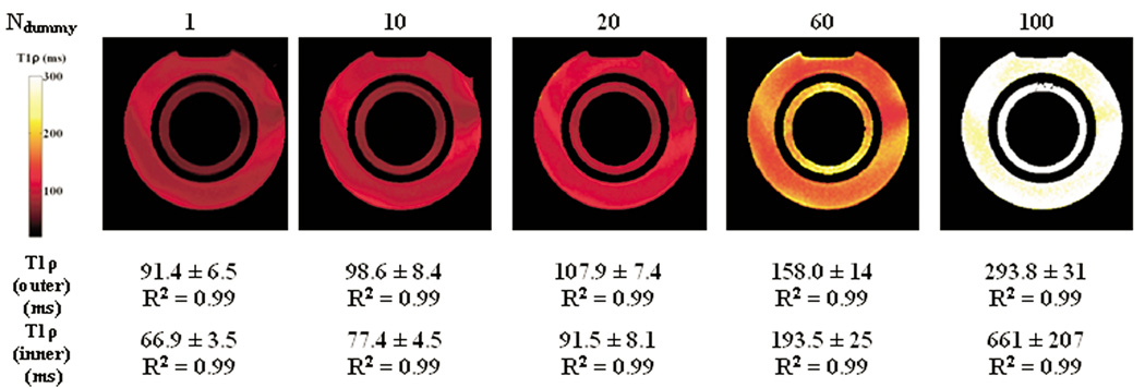
Loss of T1ρ-weighting during b-GRE acquisition illustrated by T1ρ relaxation maps and corresponding R² without transient signal filter compensation in a two compartment (cylinder within a cylinder) phantom doped with 0.025 mM MnCl₂ (Outer Compartment: T1 = 1 s, T2 = 80 ms, T1ρ = 95 ms) and 0.04 mM MnCl₂ (Inner Compartment: T1 = 600 ms, T2 = 50 ms, T1ρ = 65 ms). Actual T1ρ relaxation times were measured separately by T1ρ-prepared single echo spin echo as described in Methods. As the number of dummy pulses prior to encoding the center of k-space is increased, T1ρ relaxation times are artificially increased. B₀ field inhomogeneity at the interface between water and air compartments during the b-GRE acquisition causes T1ρ banding across the phantom.

B₀ field inhomogeneity across the two-compartment phantom causes erratic and different transient signal decay during the b-GRE sequence. These effects are noticeable across the phantoms and cause spatial variation in T1ρ across the homogeneous phantom. T1ρ enhancement at the edge of the phantoms appears in the phase encode direction and is attributed to the changing point spread function with different TSL times (Figure 2). The spatial width of the T1ρ-enhanced edge is proportional to the voxel size, so larger matrix sizes are less sensitive to this artifact. Despite the loss of T1ρ contrast, even for N_dummy = 100 we observed exponential decay with a prolonged T1ρ relaxation time (R² = 0.99).

Figure 6 corrects for blurring using the filter described above. A MnCl₂-doped water phantom (T1 = 270 ms, T2 = 40 ms, T1ρ = 45 ms) was imaged with T1ρ-prepared b-GRE (TSL = 2 ms, TR = 7.4 ms, T_DELAY = 6 s). The unfiltered and filtered images are shown and improvement in the phantom profile is clearly noticeable.

Figure 6.

Transient signal filter implemented on a MnCl₂-doped water phantom (T1 = 270 ms, T2 = 40 ms, T1ρ = 45 ms) for T_SL = 2 ms. The unfiltered image is blurred because of the transient signal decay. The filter (Figure 4D) sharpens the phantom edges and improves the phantom profile.

T1ρ-prepared b-GRE was compared with a standard T1ρ-prepared single echo spin echo pulse sequence in human patellar articular cartilage in vivo in a healthy 23 year old male. Patellar articular cartilage joint contrast for 4 TSL times and the corresponding T1ρ map is shown in Figure 7. A ROI was drawn encompassing the entire medial or lateral patellar cartilage. The medial mean patellar cartilage was 34.2 ± 4.9 (3D) and 37.7 ± 7.6 ms (2D) and the lateral mean patellar cartilage was 35.5 ± 1.8 (3D) and 36.9 ± 3.2 ms (2D). In each case, 2D and 3D T1ρ maps were in good agreement and the difference between the two T1ρ map ROIs was less than one standard deviation of the 3D map. R² for all T1ρ map regions-of-interest was greater than 0.99 and confirmed the exponential decay of magnetization.

Figure 7.

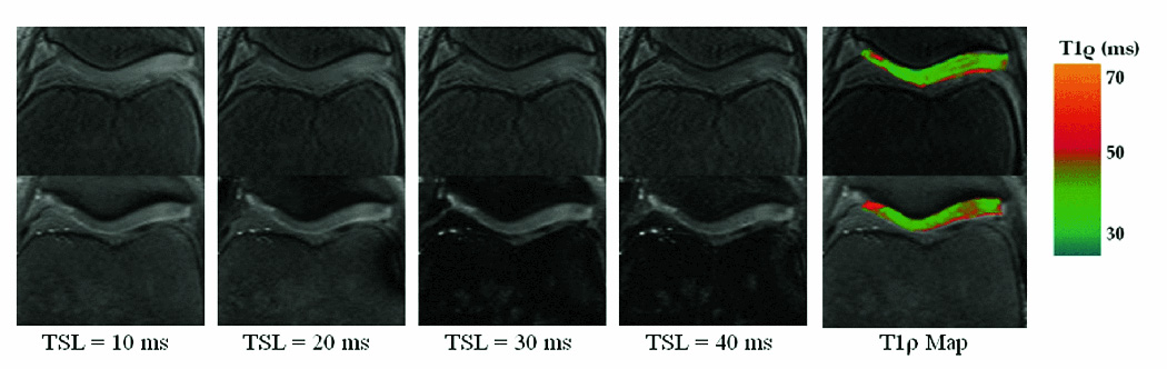
4 Axial T1ρ-weighted images of the knee patellar articular cartilage with different contrasts (TSL) for both 3D b-GRE acquisitions (top row) and 2D spin echo (bottom row). Medial mean patellar cartilage was 34.2 ± 4.9 (3D) and 37.7 ± 7.6 ms (2D). Lateral mean patellar cartilage was 35.5 ± 1.8 (3D) and 36.9 ± 3.2 ms (2D). In each case, the difference between 2D and 3D T1ρ maps was less than one standard deviation of the 3D map. R² for all T1ρ map regions-of-interest was greater than 0.99 and confirmed the exponential decay of magnetization. Blurring was corrected using the transient signal filter shown in Figure 4B with the following relaxation time estimates: T1 = 1 s, T2 = 35 ms, T1ρ = 40 ms. The white arrow in the spin echo map (T1ρ = 40.5 ± 1.0) depicts a region elevated relative to the b-GRE acquisition (T1ρ = 36.7 ± 1.1) and may reflect through-plane motion over the course of the twenty minute imaging period.

20 slice, axial T1ρ relaxation maps were obtained for a single asymptomatic subject who underwent 4 consecutive knee examinations to determine T1ρ reproducibility. 3 representative slices (slice 10, 11 and 13) from each of the 4 examinations are shown in Figure 8. T1ρ-prepared b-GRE preserves the layered appearance of T1ρ relaxation times across the cartilage from the articular surface to the subchondrol bone. It is possible to distinguish 2 cartilage layers in Figure 9 as T1ρ relaxation times increase monotonically from the subchondral bone to the superficial zone and joint space. For slices 10 and 11, where both the patellar and femoral cartilage is visible, there is an increase in T1ρ from the patella to the patellofemoral joint space, followed by decreasing T1ρ to the femoral surface. Intrasubject coregistration was performed to minimize differences between the slices between sessions, however, some differences are noticeable. For example, the femoral cartilage is visible in session 1, slice 13, but has moved out of the visible slice for the other three sessions. It may be beneficial to further reduce the slice thickness to 2–3 mm to minimize partial voluming of the T1ρ-weighted images.

Figure 8.

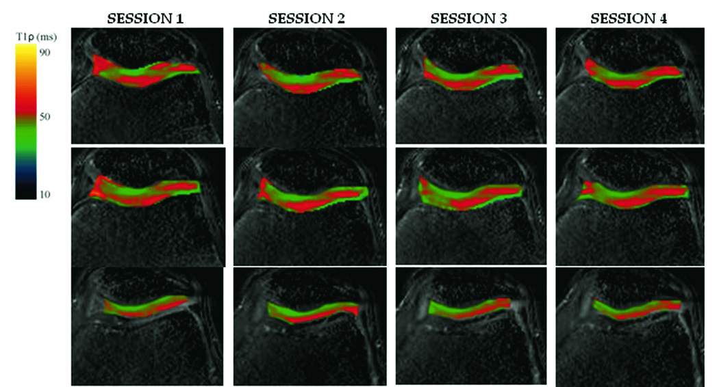
T1ρ relaxation maps overlaid on T1ρ-weighted images from one 20 year old asymptomatic subject who underwent 4 consecutive knee examinations at 1.5 T. Each examination consisted of a five T1ρ-prepared b-GRE experiment with 5 spin lock durations (TSL = 2, 10, 20, 30, 40 ms) in a 20 slice sequence. Shown here are slices 9, 11 and 13 in the series (top to bottom). The T1ρ-prepared magnetization was frequency and phase encoded using a centrically ordered b-GRE with α = 50°with an α/2 preparatory pulse followed by a single dummy pulse and 256 phase encoding lines in the right/left direction. Blurring was corrected using the transient signal filter shown in Figure 4B with the following relaxation time estimates: T1 = 1 s, T2 = 35 ms, T1ρ = 40 ms.

Figure 9.

3D lower lumbar T1ρ maps of a 23 year old asymptomatic subject. Mean T1ρ in the nucleus pulposus was 114.7 ± 9.0 ms (L1/L2), 132.6 ± 25.0 ms (L2/L3), 170.2 ± 24.9 ms (L3/L4), 146.6 ± 14.7 ms (L4/L5) and 96.6 ± 14.3 ms (L5/S1).

3D T1ρ maps of the human spine images are shown in Figure 9. The pulse sequence was modified for imaging of the spine to further reduce blurring. A segmented, centric pulse sequence was constructed (N_segment=64, N_ky = 256). To compensate for the 4-fold increase in scan duration, the pulse sequence was not inversion recovery prepared so the magnetization recovery period T_DELAY was reduced to 2 s. Mean nucleus pulposus T1ρ for each lower lumbar disc was 114.7 ± 9.0 ms (L1/L2), 132.6 ± 25.0 ms (L2/L3), 170.2 ± 24.9 ms (L3/L4), 146.6 ± 14.7 ms (L4/L5) and 96.6 ± 14.3 ms (L5/S1).

Discussion

3D T1ρ-prepared b-GRE acquisitions are able to acquire a single view (axial, coronal or sagittal) in a third the time necessary to acquire a similar 3D T1ρ-prepared GRE. The considerable time savings allows for clinical implementation of 3D T1ρ relaxation mapping in 10 minutes using the sequence designed above. The acquisition time could be further reduced through parallel processing techniques or models of T1ρ relaxation that account for T1 saturation during a shortened T_DELAY period. An inversion recovery pulse (TI = 1700 ms) was implemented in the current sequence to limit joint space fluid blurring in the adjacent cartilage, however, when blurring is not an issue the acquisition time can be further reduced so T_DELAY = 2 s. ..

Efforts to reduce blurring during the b-GRE acquisition for different TSL times are being pursued. Blurring can be reduced by variable flip angle b-GRE acquisitions designed to offset the transient signal decay during readout. A potential variable flip angle train for reducing blurring would be to monotonically increase the flip angle to offset the signal decay observed for large flip angles such as for α = 70° (Figure 2). This technique is limited since the flip angle train must be customized for a particular tissue with a known T1, T2 and T1ρ. A simple solution to implement as an alternative to this type of variable flip angle train is a kspace filter designed to compensate for the known signal decay during the b-GRE acquisition such as that shown in Figure 4. An estimate of T1, T2 and T1ρ and the resulting signal evolution such as those depicted in Figure 2 can enable the design of a filter used to compensate for the transient signal during readout. This technique is limited, however, due to unknown T1s and T2s and off-resonance spins, which may have different signal trajectories during b-GRE acquisition. Variable flip angle sequences require similar estimates of T1 and T2 to control the transient signal decay (29). In some cases, filtering, as opposed to variable flip angle acquisition, may have higher signal to noise, since variable flip angle techniques begin with a low flip angle to encode the kspace center and subsequently ramp up the flip angle.

Another variable flip angle acquisition combines T1ρ-preparation with a T2-TIDE (Transition Into Driven Equilibrium) sequence (29). T2-TIDE has the added benefit that the T2 decay during the early portion of the sequence is analogous to the T1ρ-prepared fast spin echo sequences used for single or multislice T1ρ acquisitions. The T2-TIDE acquisition will not need to be customized for a particular tissue and T1ρ parametric mapping should work equally well on the head or knee joint. T2-TIDE is limited by the blurring of the signal because of T2-decay during the initial acquisition; however, the increased signal to noise of the initial spin echo readout may be justified.

The dependency of the apparent T1ρ relaxation time on variations in the readout sequence is troublesome for consistent T1ρ quantification among different investigators. When providing T1ρ relaxation times in tissues it is necessary to specify exactly the readout sequence used for acquisition including the RF pulse flip angles, echo and repetitions times of the sequence. Small changes in any of the readout parameters can impact the resulting T1ρ measurement. Variations in T1ρ with readout are analogous to variations in T2 with multiecho or single echo acquisitions and procedures for comparing relaxation times among different investigators need to be constructed.

In conclusion, clinical examinations with 3D or multiple view coverage was not possible using current T1ρ imaging methods. To address this problem, we developed a T1ρ-prepared b-GRE acquisition technique to significantly reduce the time necessary to acquire a 3D field of view. T1ρ-prepared b-GRE was used to obtain a single 20 slice T1ρ relaxation map of the knee patellar and femoral cartilage in 10 minutes. Using T1ρ-prepared b-GRE, the T1ρ relaxation times in human patellar and femoral cartilage were reproducible. The sequence is limited, however, by competing T1ρ-weighted signal and the b-GRE transient signal decay during acquisition, which filters the k-space in the phase encoding direction. The effect of the filtering on the apparent T1ρ relaxation times and blurring was shown in phantoms and humans and a post-processing filter was developed to minimize these effects. Further, the flexibility of the sequence was shown by extension to the human spine in vivo.

References

- 1.Redfield AG. Nuclear Magnetic Resonance Saturation and Rotary Saturation in Solids. Physical Review. 1955;98(6):1787–1809. [Google Scholar]
- 2.Santyr GE, Henkelman RM, Bronskill MJ. Spin Locking for Magnetic-Resonance Imaging with Application to Human-Breast. Magnetic Resonance in Medicine. 1989;12(1):25–37. doi: 10.1002/mrm.1910120104. [DOI] [PubMed] [Google Scholar]
- 3.Kettunen MI, Kauppinen RA, Grohn OHJ. Dispersion of cerebral on-resonance T-1 in the rotating frame (T-1p) in global ischaemia. Applied Magnetic Resonance. 2005;29(1):89–106. [Google Scholar]
- 4.Grohn OHJ, Makela HI, Lukkarinen JA, et al. On- and off-resonance T-1 rho MRI in acute cerebral ischemia of the rat. Magnetic Resonance in Medicine. 2003;49(1):172–176. doi: 10.1002/mrm.10356. [DOI] [PubMed] [Google Scholar]
- 5.Wheaton AJ, Borthakur A, Kneeland JB, Regatte RR, Akella SVS, Reddy R. In vivo quantification of T-1 rho using a multislice spin-lock pulse sequence. Magnetic Resonance in Medicine. 2004;52(6):1453–1458. doi: 10.1002/mrm.20268. [DOI] [PubMed] [Google Scholar]
- 6.Lozano J, Li XJ, Link TA, Safran M, Majumdar S, Ma CB. Detection of posttraumatic cartilage injury using quantitative T1Rho magnetic resonance imaging - A report of two cases with arthroscopic findings. Journal of Bone and Joint Surgery-American Volume. 2006;88A(6):1349–1352. doi: 10.2106/JBJS.E.01051. [DOI] [PubMed] [Google Scholar]
- 7.Auerbach JD, Johannessen W, Borthakur A, et al. In vivo quantification of human lumbar disc degeneration using T-1 rho-weighted magnetic resonance imaging. European Spine Journal. 2006;15:S338–S344. doi: 10.1007/s00586-006-0083-2. [DOI] [PMC free article] [PubMed] [Google Scholar]
- 8.Johannessen W, Auerbach JD, Wheaton AJ, et al. Assessment of human disc degeneration and proteoglycan content using T-1p-weighted magnetic resonance imaging. Spine. 2006;31(11):1253–1257. doi: 10.1097/01.brs.0000217708.54880.51. [DOI] [PMC free article] [PubMed] [Google Scholar]
- 9.Borthakur A, Hulvershorn J, Gualtieri E, et al. A pulse sequence for rapid in vivo spin-locked MRI. Journal of Magnetic Resonance Imaging. 2006;23(4):591–596. doi: 10.1002/jmri.20537. [DOI] [PMC free article] [PubMed] [Google Scholar]
- 10.Hulvershorn J, Borthakur A, Bloy L, et al. T-1 rho contrast in functional magnetic resonance imaging. Magnetic Resonance in Medicine. 2005;54(5):1155–1162. doi: 10.1002/mrm.20698. [DOI] [PMC free article] [PubMed] [Google Scholar]
- 11.Charagundla SR, Duvvuri U, Noyszewski EA, et al. O-17-decoupled H-1 spectroscopy and imaging with a surface coil: STEAM decoupling. Journal of Magnetic Resonance. 2000;143(1):39–44. doi: 10.1006/jmre.1999.1948. [DOI] [PubMed] [Google Scholar]
- 12.Tailor DR, Poptani H, Glickson JD, Leigh JS, Reddy R. High-resolution assessment of blood flow in murine RIF-1 tumors by monitoring uptake of (H2O)-O-17 with proton T-1 rho-weighted imaging. Magnetic Resonance in Medicine. 2003;49(1):1–6. doi: 10.1002/mrm.10375. [DOI] [PubMed] [Google Scholar]
- 13.Tailor DR, Roy A, Regatte RR, et al. Indirect O-17-magnetic resonance imaging of cerebral blood flow in the rat. Magnetic Resonance in Medicine. 2003;49(3):479–487. doi: 10.1002/mrm.10403. [DOI] [PubMed] [Google Scholar]
- 14.Solomon I. Rotary Spin Echoes. Physical Review Letters. 1959;2(7):301–302. [Google Scholar]
- 15.Charagundla SR, Borthakur A, Leigh JS, Reddy R. Artifacts in T-1 rho-weighted imaging: correction with a self-compensating spin-locking pulse. Journal of Magnetic Resonance. 2003;162(1):113–121. doi: 10.1016/s1090-7807(02)00197-0. [DOI] [PubMed] [Google Scholar]
- 16.Witschey WRTBA, II, Elliott MA, Mellon E, Niyogi S, Wallman DJ, Wang C, Reddy R. Artifacts in T1rho-weighted imaging: Compensation for B1 and B0 field imperfections. Journal of Magnetic Resonance. 2007;186:75–85. doi: 10.1016/j.jmr.2007.01.015. [DOI] [PMC free article] [PubMed] [Google Scholar]
- 17.Santyr GE, Fairbanks EJ, Kelcz F, Sorenson JA. Off-Resonance Spin Locking for Mr-Imaging. Magnetic Resonance in Medicine. 1994;32(1):43–51. doi: 10.1002/mrm.1910320107. [DOI] [PubMed] [Google Scholar]
- 18.Grohn HI, Michaeli S, Garwood M, Kauppinen RA, Grohn OHJ. Quantitative T-1p and adiabatic Carr-Purcell T-2 magnetic resonance imaging of human occipital lobe at 4 T. Magnetic Resonance in Medicine. 2005;54(1):14–19. doi: 10.1002/mrm.20536. [DOI] [PubMed] [Google Scholar]
- 19.Li XJ, Han ET, Ma CB, Link TM, Newitt DC, Majumdar S. In vivo 3T spiral imaging based multi-slice T-1p mapping of knee cartilage in osteoarthritis. Magnetic Resonance in Medicine. 2005;54(4):929–936. doi: 10.1002/mrm.20609. [DOI] [PubMed] [Google Scholar]
- 20.Borthakur A, Wheaton A, Charagundla SR, et al. Three-dimensional T1 rho-weighted MRI at 1.5 Tesla. Journal of Magnetic Resonance Imaging. 2003;17(6):730–736. doi: 10.1002/jmri.10296. [DOI] [PubMed] [Google Scholar]
- 21.Diemling MHO. Magnetization prepared true FISP imaging. San Francisco: 1994. p. 495. [Google Scholar]
- 22.Scheffler K, Hennig J. T-1 quantification with inversion recovery TrueFISP. Magnetic Resonance in Medicine. 2001;45(4):720–723. doi: 10.1002/mrm.1097. [DOI] [PubMed] [Google Scholar]
- 23.Scheffler K. On the transient phase of balanced SSFP sequences. Magnetic Resonance in Medicine. 2003;49(4):781–783. doi: 10.1002/mrm.10421. [DOI] [PubMed] [Google Scholar]
- 24.Scheffler K, Lehnhardt S. Principles and applications of balanced SSFP techniques. European Radiology. 2003;13(11):2409–2418. doi: 10.1007/s00330-003-1957-x. [DOI] [PubMed] [Google Scholar]
- 25.Bernstein MA, King KF, Zhou ZJ. Handbook of MRI pulse sequences. xxii. Burlington, MA: Elsevier Academic Press; 2004. 1017 pp. [Google Scholar]
- 26.Boos N, Wallin A, Schmucker T, Aebi M, Boesch C. Quantitative Mr-Imaging of Lumbar Intervertebral Disks and Vertebral Bodies - Methodology, Reproducibility, and Preliminary-Results. Magnetic Resonance Imaging. 1994;12(4):577–587. doi: 10.1016/0730-725x(94)92452-x. [DOI] [PubMed] [Google Scholar]
- 27.Mugler JP, Brookeman JR. 3-Dimensional Magnetization-Prepared Rapid Gradient-Echo Imaging (3Dmp-Rage) Magnetic Resonance in Medicine. 1990;15(1):152–157. doi: 10.1002/mrm.1910150117. [DOI] [PubMed] [Google Scholar]
- 28.Collins CM, Li SZ, Smith MB. SAR and B-1 field distributions in a heterogeneous human head model within a birdcage coil. Magnetic Resonance in Medicine. 1998;40(6):847–856. doi: 10.1002/mrm.1910400610. [DOI] [PubMed] [Google Scholar]
- 29.Paul D, Markl M, Fautz HP, Hennig J. T-2-weighted balanced SSFP imaging (T-2-TIDE) using variable flip angles. Magnetic Resonance in Medicine. 2006;56(1):82–93. doi: 10.1002/mrm.20922. [DOI] [PubMed] [Google Scholar]