Abstract
A method was proposed for the detection of outliers and influential observations in the framework of a mixed linear model, prior to the quantitative trait locus (QTL) mapping analysis. We investigated the impact of outliers on QTL mapping for complex traits in a mouse BXD population, and observed that the dropping of outliers could provide the evidence of additional QTL and epistatic loci affecting the 1stBrain-OB and the 2ndBrain-OB in a cross of the abovementioned population. The results could also reveal a remarkable increase in estimating heritabilities of QTL in the absence of outliers. In addition, simulations were conducted to investigate the detection powers and false discovery rates (FDRs) of QTLs in the presence and absence of outliers. The results suggested that the presence of a small proportion of outliers could increase the FDR and hence decrease the detection power of QTLs. A drastic increase could be obtained in the estimates of standard errors for position, additive and additive×environment interaction effects of QTLs in the presence of outliers.
Keywords: QTL mapping, Outliers and influential observations, Complex trait
INTRODUCTION
With the advent of molecular technology and the availability of highly dense genetic markers, the problem of mapping quantitative trait locus (QTL) for complex traits is now well established. Many statistical methodologies have been developed to cope with the situation (Lander and Botstein, 1989; Haley and Knott, 1992; Zeng, 1994; Wang et al., 1999). All these methods have been extensively applied in plant and animal breeding experiments for QTL mapping analyses to obtain the genomic positions of individual QTLs and their estimated effects in an authentic framework. Each method requires the availability of genetic markers, a genetic map and phenotype data of an experimental population. However, in reality these datasets often contain outliers and influential observations (Pérez-Enciso and Toro, 1999) that may seriously affect the estimates of model parameters and can lead to the wrong detection of QTL positions and their estimated effects (Fernandes et al., 2007). The presence of outliers in the phenotype data can incorrectly indicate multiple linked QTLs and may hinder the efficient and accurate resolvability of QTLs (Jansen and Stam, 1994). Therefore, it is important that a researcher or data analyst have some prior knowledge about the spectrum of data, possibly for unusual data points and their influence on the results of the analysis.
Outliers are the most noteworthy data points and their identification can lead to the development of a better genetic model. The influence diagnostic analysis is necessary in the modeling schemes for identifying the hidden peculiarities which have an exceedingly large influence on the estimated parameters of the fitted model (Schabenberger, 2004). In the present study, methods for the identification of outliers and influential observations are presented in the framework of a linear mixed model prior to the QTL mapping analysis. We investigated the influence of outliers on QTLs controlling complex traits in a mouse BXD population. The advantages and disadvantages of outliers influence on the detection of QTLs and their estimated effects were discussed. In addition, we also investigated the detection powers and false discovery rates (FDRs) of QTLs in the presence and absence of outliers using simulations.
MATERIALS AND METHODS
Materials
The dataset was downloaded from the Web (http://www.nervenet.org/main/databases.html). The data was collected from a recombinant inbred (RI) strain derived from a cross between two ancestor inbred strains, C57BL/6J and DBA/2J (BXD). The BXD population consists of 35 strains with 390 animals. The genetic linkage map covers a range of 20 chromosomes (19 autosomes and 1 sex chromosome) with 1 095 markers. It spans 2 037.6 cM of the mouse genome with an average distance of 1.86 cM between two markers. Two different traits, 1stBrain-OB and 2ndBrain-OB, were used to demonstrate the procedure and to check the influence of outliers on the QTL mapping results. The phenotypic data has the logarithm of mice age which was adjusted by the residual analysis through a regression approach by conditioning a trait on the logarithm of mice age. This correction was made for both the traits to exclude the effect of the logarithm of age (Williams et al., 2001). The effect of sex was considered as an environmental factor in the model of QTL mapping analysis.
QTL mapping
Two different approaches were used to analyze the data in the framework of a mixed linear model. The first approach deals with QTL mapping using the software QTLNetwork 2.0 (Yang et al., 2007) at a 5% genome-wise significance level, while the second method was used for the detection of outliers and influential observations. After the outlier analysis, unusual data points were removed from the data and the data was re-analyzed to map QTLs by the aforementioned software. When analyzing the data for QTLs affecting 1stBrain-OB and 2ndBrain-OB in the mouse BXD population, the Henderson method-III (Searle et al., 1992) was used to construct the F-statistic profile along the genome, separated by 1 cM for each 1D and 2D genome scan strategies. The 1D genome scan was used for detecting QTLs with additive (a) and/or additive×environment (sex) (ae) interaction effects, while additive×additive (aa) epistatic loci and/or their interaction with sex (aae) were determined by 2D genome scan procedure. In both the 1D and 2D scan strategies, the F-threshold values were calculated by 1 000 permutation tests (Doerge and Churchill, 1996) to control the genome-wide type-I error rate. When any of the F-statistic values for a region exceeded the F-threshold, a QTL at that position with the regional maximum F-value was declared as an identified QTL. The significance of QTLs with a, ae, aa and aae effects was estimated and tested by the Markov Chain Monte Carlo (MCMC) method via Gibbs sampling (Yang et al., 2007).
Furthermore, to check the influence of outliers on the detection powers and FDRs of QTLs, 200 simulations were conducted by using the strategy described by Yang et al.(2007). Five QTLs (Q 1, Q 2, …, Q 5) with additive (a) and/or additive×environment interaction (ae) effects were located on five different chromosomes. The dataset consisting of 200 double-haploid lines (DHLs) evaluated in two different environments constituted a total of 400 observations. A genetic linkage map containing five chromosomes each having the length of 100 cM with 11 equally spaced genetic markers was used in the simulation. The detailed information regarding various parameters (position, a and ae effects of QTLs) is listed in Table 4 (in the section of RESULTS). Simulations were conducted in four different ways, i.e., the dataset having no outliers (clean data) and the datasets containing 1%, 5%, and 10% of outliers. Outliers were incorporated in the phenotype data by adding a small positive value after generating the clean data, throughout the simulations.
Table 4.
Summarized results of QTL with additive (a) and additive×environment (ae) interaction effects from 200 simulated data having no outlier, or 1%, 5% and 10% outliers
| Chr | Pos (cM) |
SI width (cM) |
a |
ae1 |
ae2 |
||||||
| TV | Est (SE) | TV | Est (SE) | TV | Est (SE) | TV | Est (SE) | ||||
| No outlier | Q1 | 1 | 44 | 44.23 (3.14) | 12.1 | –2.78 | –2.71 (0.42) | 0 | 0.01 (0.28) | 0 | –0.01 (0.28) |
| Q2 | 2 | 75 | 74.85 (4.83) | 17.3 | 0 | –0.03 (0.48) | –1.7 | –1.83 (0.35) | 1.7 | 1.85 (0.36) | |
| Q3 | 3 | 50 | 49.74 (1.91) | 9.0 | 2.90 | 2.97 (0.42) | –1.6 | –1.53 (0.43) | 1.6 | 1.55 (0.44) | |
| Q4 | 4 | 73 | 73.29 (2.67) | 9.7 | –3.30 | –3.27 (0.42) | 0 | –0.01 (0.27) | 0 | 0.01 (0.27) | |
| Q5 | 5 | 15 | 14.70 (4.89) | 17.0 | 1.90 | 2.02 (0.37) | 0 | 0.03 (0.30) | 0 | –0.03 (0.30) | |
| 1% outliers | Q1 | 1 | 44 | 43.99 (3.45) | 13.2 | –2.78 | –2.74 (0.47) | 0 | –0.00 (0.34) | 0 | 0.00 (0.34) |
| Q2 | 2 | 75 | 74.41 (5.58) | 18.2 | 0 | –0.01 (0.49) | –1.7 | –1.97 (0.43) | 1.7 | 2.01 (0.46) | |
| Q3 | 3 | 50 | 49.85 (2.00) | 9.8 | 2.90 | 3.00 (0.48) | –1.6 | –1.51 (0.51) | 1.6 | 1.53 (0.52) | |
| Q4 | 4 | 73 | 73.32 (3.34) | 11.5 | –3.30 | –3.27 (0.48) | 0 | –0.01 (0.32) | 0 | 0.01 (0.32) | |
| Q5 | 5 | 15 | 14.77 (4.45) | 16.6 | 1.90 | 2.16 (0.44) | 0 | 0.06 (0.32) | 0 | –0.06 (0.32) | |
| 5% outliers | Q1 | 1 | 44 | 44.41 (4.13) | 16.6 | –2.78 | –2.91 (0.52) | 0 | –0.02 (0.42) | 0 | 0.02 (0.42) |
| Q2 | 2 | 75 | 74.12 (5.46) | 18.5 | 0 | –0.28 (0.74) | –1.7 | –2.31 (0.72) | 1.7 | 2.36 (0.77) | |
| Q3 | 3 | 50 | 49.84 (2.59) | 12.4 | 2.90 | 3.00 (0.62) | –1.6 | –1.41 (0.73) | 1.6 | 1.41 (0.73) | |
| Q4 | 4 | 73 | 73.32 (4.07) | 14.2 | –3.30 | –3.38 (0.56) | 0 | –0.05 (0.42) | 0 | 0.05 (0.42) | |
| Q5 | 5 | 15 | 14.63 (5.61) | 17.2 | 1.90 | 2.46 (0.63) | 0 | 0.22 (0.48) | 0 | –0.21 (0.47) | |
| 10% outliers | Q1 | 1 | 44 | 44.31 (4.66) | 16.4 | –2.78 | –3.04 (0.59) | 0 | –0.01 (0.35) | 0 | 0.02 (0.35) |
| Q2 | 2 | 75 | 73.09 (5.93) | 19.9 | 0 | –0.64 (1.02) | –1.7 | –2.29 (0.68) | 1.7 | 2.32 (0.72) | |
| Q3 | 3 | 50 | 49.90 (2.29) | 12.4 | 2.90 | 3.06 (0.71) | –1.6 | –1.35 (0.73) | 1.6 | 1.35 (0.73) | |
| Q4 | 4 | 73 | 73.73 (4.07) | 13.9 | –3.30 | –3.39 (0.61) | 0 | –0.02 (0.34) | 0 | 0.02 (0.34) | |
| Q5 | 5 | 15 | 14.00 (5.46) | 15.6 | 1.90 | 2.72 (0.89) | 0 | 0.25 (0.52) | 0 | –0.24 (0.51) | |
Chr: chromosome number; Pos: position of QTL Qi (i=1,2,3,4,5); TV: True value; Est (SE): estimate (standard error); SI width: the length of support interval; a: additive effect of QTL; ae 1 and ae 2: interaction of QTL having additive effect with ith environment (i=1, 2)
Detecting outliers and influential observations
An observation is defined to be an outlier when having a large residual as compared with rest of the observations of a dataset. Zewotir and Galpin (2007) defined that an observation will be an outlier if  and
and  max|ti|>t
(1−α/n;n−p−1), or if max|ti|>t
(1−α/n;n−rank|XU|) (SAS, 1999), where, ti is the studentized residual obtained by MINQUE (1) via linear unbiased prediction (LUP) (Zhu and Weir, 1994a; 1994b), i.e.,
  with
with  and
and  being the estimated residual for the ith observation; X and U are the known coefficient matrices associated with the fixed effect vector b and the random effect vector e of a mixed linear model, respectively; Q
(1) is a symmetric matrix; and V is the variance-covariance matrix (Zhu, 1997). In the present study we calculate the P-value of each observation from its corresponding t-value and define an observation as an outlier if Pi<P
cutoff (i=1,2,…,n), where P
cutoff is calculated by the FDR method (Benjamini and Hochberg, 1995).
For the detection of influential observations, the Zewotir and Galpin (2005)’s approach was adopted in the framework of MINQUE (1) via LUP, and an analogue of the Cook (1977)’s distance statistic was used for the identification of influential observations, which can be defined as:
 , ,
|
(1) |
 , ,
|
(2) |
where, p is the number of parameters to be estimated; v̂ii is the ith diagonal element of the inverse of variance-covariance matrix (V
−1); ti is the studentized residual (externally) for the ith data point; Q̂ii is the main diagonal element of matrix Q^ for the ith data point;  is the estimated residual variance; b^ is the vector of fixed effect parameter’s estimates; b^(i) is the vector of fixed effect parameter’s estimates without the ith observation; e^ is the vector of random effect parameter’s estimates; e^(i) is the vector of random effect parameter’s estimates without outliers; D is the variance-covariance matrix of the random factors; and ssq(Q^)i (i=1,2,…,n) is the sum of squares of the elements of the ith column of Q matrix (Q
(1)). Generally, large values of CDi(b) and CDi(e) (i=1,2,…,n) will flag the points which exert large influence on the fixed and random effect parameter estimates of a mixed linear model, respectively (Zewotir and Galpin, 2005).
RESULTS
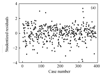
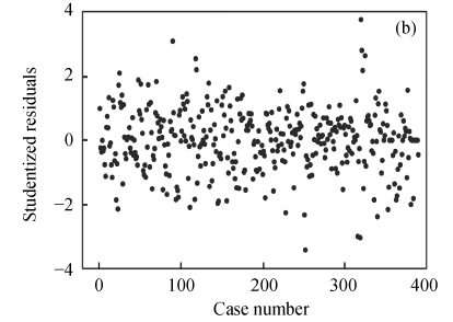
To map QTLs affecting the 1stBrain-OB and the 2ndBrain-OB in the mouse BXD population, the data were analyzed in two different ways, i.e., with and without outliers. The index plot of studentized residuals for the 1stBrain-OB and the 2ndBrain-OB was presented in Fig.1.
Fig. 1.
Index plot of studentized residuals for the phenotypes of 1stBrain-OB (a) and 2ndBrain-OB (b) in the mouse BXD population
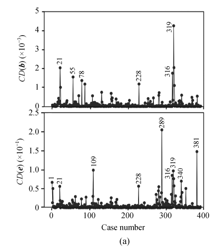
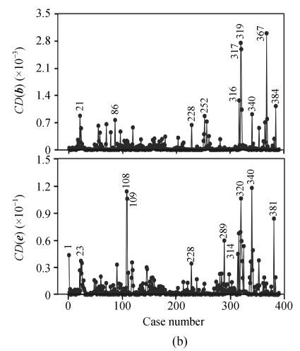
For both of the traits, the values of studentized residuals are more scattered, which provides the indication of outliers (P<0.05). It revealed that the studentized residuals for each of the phenotype values are lying in the range of ±4SD (standard deviation). Studentized residual analysis resolved the existence of 4.36% of outliers in both of the traits, respectively. In a similar way, very few influential observations in the 1stBrain-OB were observed but their existence was large in the 2ndBrain-OB, influencing the fixed and random components of the fitted model (Fig.2).
Fig. 2.
Influence diagnostic plots of CD(b) and CD(e) affecting the fixed and random effects of a linear mixed model, respectively, for the 1stBrain-OB (a) and the 2ndBrain-OB (b) of the mouse BXD population
The results regarding QTLs affecting the 1stBrain-OB and the 2ndBrain-OB with and without outliers and influential observations are listed in Table 1. Prior to the outliers and influence analysis, two and three QTLs were detected, respectively, for the 1stBrain-OB and 2ndBrain-OB. The two QTLs affecting the 1stBrain-OB were located on chromosomes 15 and 19 with positive additive effects. In a similar way, the three QTLs associated with the 2ndBrain-OB were observed on chromosomes 4, 11, and 13. The individual effect of QTL on chromosome 4 was negative while others showed positive effects. When outliers were removed from the phenotype data (clean data), one additional QTL on chromosome 15 was detected for controlling the 1stBrain-OB and three additional QTL were recorded for the 2ndBrain-OB. No QTL showed interaction with sex in either case (with and without outliers) affecting the studied traits. However, one pair of epistatic loci was detected for the 2ndBrain-OB, explaining a small amount of phenotype variation (Table 2). In addition, remarkable changes were obtained in estimating the proportion of variance components for the clean datasets of both the phenotypes (Table 3).
Table 1.
QTL affecting the 1stBrain-OB and the 2ndBrain-OB in the mouse BXD population with and without outliers and influential observations
| Trait | QTL | SI (cM) | a | h(a)2 (%) | |
| With outliers | 1stBrain-OB | 1stb15-35 | 71.2~73.6 | 7.354 (1.206)* | 6.63 |
| 1stb19-11 | 10.0~11.9 | 10.017 (1.189) | 14.21 | ||
| 2ndBrain-OB | 2ndb4-61 | 97.6~99.5 | −8.122 (1.361) | 5.61 | |
| 2ndb11-7 | 6.3~9.6 | 7.088 (1.361) | 8.39 | ||
| 2ndb13-16 | 42.7~49.5 | 9.449 (1.399) | 7.92 | ||
| Without outliers | 1stBrain-OB | 1stb15-32 | 68.7~69.9 | 7.251 (1.047) | 8.11 |
| 1stb19-11 | 10.0~11.9 | 9.474 (1.047) | 16.51 | ||
| 2ndBrain-OB | 2ndb2-78 | 93.3~96.8 | 12.615 (1.183) | 7.80 | |
| 2ndb8-23 | 38.0~41.5 | −10.148 (1.183) | 12.72 | ||
| 2ndb11-12 | 10.7~15.2 | 8.236 (1.204) | 9.32 | ||
QTL expressed as trait name (1stb and 2ndb) followed by the chromosome number and the marker interval separated by hyphen; SI: the support interval of a QTL; a: the additive effect of a QTL; h (a) 2: the heritability (phenotypic variation) explained by the QTL with additive (a) effect
The values in brackets show the standard errors (SE);
Table 2.
QTLs with additive×additive (aa) epistasis effect
| Trait | QTL1 | SI1 (cM) | QTL2 | SI2 (cM) | aa | h(aa)2 (%) |
| 2ndBrain-OB | 2ndb4-8 | 8.5~13.3 | 2ndb7-6 | 5.2~12.7 | 4.81 (1.183)* | 2.70 |
SI 1 and SI 2: the support intervals of QTL1 and QTL2, respectively; h (aa) 2: the phenotype variation explained by the QTLs having aa effects;
The value in brackets is the standard error of aa epistasis effect
Table 3.
Estimates of proportion of variance components (%) for 1stBrain-OB and 2ndBrain-OB with and without outliers in the mouse BXD population
| Trait | VG/VP | VE/VP | VGE/VP | Vε/VP | |
| With outliers | 1stBrain-OB | 20.84 | 0.07 | 0.53 | 78.55 |
| 2ndBrain-OB | 21.92 | 0.03 | 1.48 | 76.57 | |
| Without outliers | 1stBrain-OB | 24.61 | 0.40 | 0.15 | 74.83 |
| 2ndBrain-OB | 32.54 | 0.08 | 1.34 | 66.04 | |
V G, V P, V E, V GE, and Vε are the variances explained by the genotype (G), phenotype (P), environment (E), genotype×environment (G×E) interaction and the residual error (ε), respectively
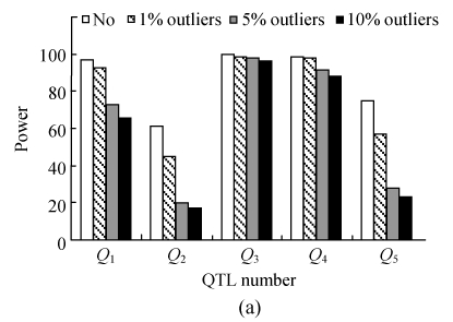
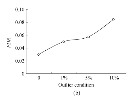
Fig.3 indicates the detection powers and false discovery rates of QTLs in the presence and absence of outliers for the simulated data. It is evident that outliers could severely affect the detection powers (Fig.3a) and increase the FDR (Fig.3b) of putative QTLs when outliers were present in the data. An increasing trend for FDR was observed with the increase in the percentage of outliers, and hence the detection power of QTLs decreases. For example, an increase of 5.55% FDR was recorded when 10% of outliers were present in the data. A drastic decrease was obvious in the estimates of standard errors for position, a and ae effects of QTLs in the presence of outliers. In addition, the lengths of support intervals of QTL positions were larger in the presence of outliers as compared with those in the absence of outliers (Table 4).
Fig. 3.
QTL detection power (a) and the false discovery rates (b) from 200 replicates of the simulated data
DISCUSSION
Identification of outliers and influential observations is important in obtaining improved estimates of the parameters and various statistical tests involved in a model (Hayat et al., 2007). Little is known about the influence of outliers in QTL mapping analysis (Jansen and Stam, 1994). In the present investigation, a series of simulations for the clean data and the datasets with outliers were performed to study the detection powers and FDRs of QTL. It was observed that the powers (or FDRs) of QTL detection could be increased (or decreased) if the dataset had no outliers. It indicated the indirect proportionality of QTL detection powers with a percentage of outliers present in the data and their direct relationship with the FDRs (Fig.3). On the other hand, smaller standard errors for various estimated effects (position, a and ae effects) of QTLs and the lengths of support intervals could be obtained in the absence of outliers (Table 4).
Cheng et al.(2003) adopted a simple approach to detect outliers in the linkage analysis on a body mass index from the Framingham heart study and the data for complex diseases and related cardiovascular risk factors. But our approach could be used in a mixed modeling framework and detect outliers in terms of their significance (P-values). We detected 4.36% of outliers and influential observations in either of the 1stBrain-OB and 2ndBrain-OB of the BXD RIL (recombinant inbred lines) mice population. Removal of outliers and influential data points brought substantial change in the identification of QTLs and their estimated effects. It suggests that outliers and influential observations can largely affect the chromosomal locations as well as their estimated effects (Cheng et al., 2003). Tilquin et al.(2001) argued that outliers contribute excessively to the residual variation, and hence decrease the detection power of QTL while using a parametric approach. A drastic decrease in the residual variance was observed when outliers and the influential phenotypes were removed from the 2ndBrain-OB, but this decrease was not so large in the phenotypes of the 1stBrain-OB values.
It is interesting to mention that one pair of epistatic loci were detected when outliers and influential observations were removed from the data of the 2ndBrain-OB. In addition, none of the two epistatic QTLs were detected with significant individual effects. However, the effect of epistatic loci was smaller (explaining 2.70% of the phenotype variation) and also showed no significant interaction to environments (sex). It indicates that epistatic interaction from modifier loci could be a common type of epistasis (Yang et al., 2007) which could act as modifying agents activating the effect of other loci (Cao et al., 2001). Li et al.(2001) suggested the achievement of local adaptation and the primary genetic basis of inbreeding depression and heterosis by strong epistasis in the fitness traits of a rice population. Williams et al.(2001) performed a detailed study for genetic dissection of the olfactory bulbs in the same BXD population and detected that four chromosomes (QTL) modulate the bulb size. However, none of the QTLs affecting bulb size were detected for both of the studied traits in either case (with and without outliers), which suggest that they could not share any of the QTL with the 1stBrain-OB and the 2ndBrain-OB.
In the present study, we performed outliers and influence analysis to investigate their effects on QTLs affecting the traits of interest. Outlier analysis tends to decompose the phenotypic variation more powerfully into genetic, environmental and other sources of variations, thus improving the accuracy of QTL and their estimated effects (Jansen and Stam, 1994). The current study throws light on the importance of clean datasets in regard to the detection of additional QTLs, with individual effects controlling the 1stBrain-OB and the 2ndBrain-OB, and additive×additive epistatic loci (Tables 1 and 2), and increasing the QTL detection powers or decreasing the FDRs (Fig.3). We are mindful that such types of studies will need extra computational load and time while performing millions of tests for the evidence of QTL and/or their interactions in the whole genome, utilizing a real dataset. However, it will increase our confidence to obtain those QTLs whose effects can be masked by outlying phenotypes in a dataset, as detected in the present investigation. An outlier may or may not be influential (Hadi and Simonoff, 1993) and here we have not considered the effect of only influential observations on the QTLs affecting the 1stBrain-OB and the 2ndBrain-OB. However, influential observations, if they exist in the phenotype data, could have a substantial impact on the estimates of various parameters and statistical tests involved in a model (our unpublished results).
Footnotes
Project supported by the National Basic Research Program (973) of China (No. 2004CB117306) and the Hi-Tech Research and Development Program (863) of China (No. 2006AA10A102)
References
- 1.Benjamini Y, Hochberg Y. Controlling the false discovery rate: a practical and powerful approach to multiple testing. J R Stat Soc Ser B. 1995;57:289–300. [Google Scholar]
- 2.Cao GQ, Zhu J, He CX, Gao YM, Wu P. Study on epistatic effects and QTL×environment interaction effects of QTLs for panicle length in rice (Oryza sativa L.) J Zhejiang Univ (Agric & Life Sci) 2001;27(1):55–61. [Google Scholar]
- 3.Cheng R, Park N, Hodge SE, Juo SHH. Comparison of the linkage results of two phenotypic constructs from longitudinal data in the Framingham Heart Study: analyses on data measured at three time points and on the average of three measurements. BMC Genet. 2003;4(Suppl. 1):S20. doi: 10.1186/1471-2156-4-S1-S20. [DOI] [PMC free article] [PubMed] [Google Scholar]
- 4.Cook RD. Detection of influential observations in linear regression. Technometrics. 1977;19(1):15–18. doi: 10.2307/1268249. [DOI] [Google Scholar]
- 5.Doerge RW, Churchill GA. Permutation tests for multiple loci affecting a quantitative character. Genetics. 1996;142:285–294. doi: 10.1093/genetics/142.1.285. [DOI] [PMC free article] [PubMed] [Google Scholar]
- 6.Fernandes E, Pacheco A, Penha-Gonçalves C. Mapping of quantitative trait loci using the skew-normal distribution. J Zhejiang Univ Sci B. 2007;8(11):792–801. doi: 10.1631/jzus.2007.B0792. [DOI] [PMC free article] [PubMed] [Google Scholar]
- 7.Hadi AS, Simonoff JS. Procedures for the identification of multiple outliers in linear models. J Am Stat Assoc. 1993;88(424):1264–1272. doi: 10.2307/2291266. [DOI] [Google Scholar]
- 8.Haley CS, Knott SA. A simple regression method for mapping quantitative trait loci in line crosses using flanking marker. Heredity. 1992;69:315–324. doi: 10.1038/hdy.1992.131. [DOI] [PubMed] [Google Scholar]
- 9.Hayat Y, Salahuddin , Mahmood Q, Islam E, Yang J. Comparative study of outliers based on statistical methods to evaluate and select the optimum regression model for fertilizers utilization. Scientific Research Monthly. 2007;3:81–84. [Google Scholar]
- 10.Jansen RC, Stam P. High resolution of quantitative traits into multiple loci via interval mapping. Genetics. 1994;136:1447–1455. doi: 10.1093/genetics/136.4.1447. [DOI] [PMC free article] [PubMed] [Google Scholar]
- 11.Lander ES, Botstein D. Mapping Mendelian factors underlying quantitative traits using RFLP linkage maps. Genetics. 1989;121(1):185–199. doi: 10.1093/genetics/121.1.185. [DOI] [PMC free article] [PubMed] [Google Scholar]
- 12.Li ZK, Luo LJ, Mei HW, Wang DL, Shu QY, Tabien R, Zhong DB, Ying CS, Stansel JW, Khush GS, et al. Over-dominant epistatic loci are the primary genetic basis of inbreeding depression and heterosis in rice. I. Biomass and grain yield. Genetics. 2001;158:1737–1753. doi: 10.1093/genetics/158.4.1737. [DOI] [PMC free article] [PubMed] [Google Scholar]
- 13.Pérez-Enciso M, Toro MA. Robust QTL effect estimation using the Minimum Distance method. Heredity. 1999;83(3):347–353. doi: 10.1038/sj.hdy.6885800. [DOI] [PubMed] [Google Scholar]
- 14.SAS. SAS STAT User’s Guide. Cary, NC, USA: SAS Institute Inc; 1999. p. 2118. Versions 7 and 8. [Google Scholar]
- 15.Schabenberger O. Mixed Model Influence Diagnostics; Proceedings of the twenty-Ninth Annual SAS Users Group International Conference; May 9-12; Montreal. Cary, NC, USA: SAS Institute Inc; 2004. pp. 1–17. Paper 189-29. [Google Scholar]
- 16.Searle SR, Casella G, McCulloch CE. Variance Components. New York: John Wiley & Sons; 1992. [Google Scholar]
- 17.Tilquin P, Coppieters W, Elsen JM, Lantier F, Moreno C, Baret PV. Statistical powers of QTL mapping methods applied to bacteria counts. Genet Res Camb. 2001;78:303–316. doi: 10.1017/s0016672301005365. [DOI] [PubMed] [Google Scholar]
- 18.Wang DL, Zhu J, Li ZK, Paterson HA. Mapping QTLs with epistatic effects and QTL×environment interactions by mixed linear model approaches. Theor Appl Genet. 1999;99(7-8):1255–1264. doi: 10.1007/s001220051331. [DOI] [Google Scholar]
- 19.Williams RW, Airey DC, Kulkarni A, Zhou G, Lu L. Genetic dissection of the olfactory bulbs of mice: QTLs on four chromosomes modulate bulb size. Behav Genet. 2001;31(1):61–77. doi: 10.1023/A:1010209925783. [DOI] [PubMed] [Google Scholar]
- 20.Yang J, Zhu J, William R. Mapping genetic architecture of complex trait in experimental populations. Bioinformatics. 2007;23(12):1527–1536. doi: 10.1093/bioinformatics/btm143. [DOI] [PubMed] [Google Scholar]
- 21.Zeng ZB. Precision mapping of quantitative traitloci. Genetics. 1994;136:1457–1468. doi: 10.1093/genetics/136.4.1457. [DOI] [PMC free article] [PubMed] [Google Scholar]
- 22.Zewotir T, Galpin JS. Influence diagnostics for linear mixed model. J Data Sci. 2005;3:153–177. [Google Scholar]
- 23.Zewotir T, Galpin JS. A unified approach on residuals, leverages and outliers in the linear mixed model. Test. 2007;16(1):58–75. doi: 10.1007/s11749-006-0001-2. [DOI] [Google Scholar]
- 24.Zhu J. Analysis Methods for Genetic Models. Beijing: Agricultural Publication House of China; 1997. p. 160. (in Chinese) [Google Scholar]
- 25.Zhu J, Weir BS. Analysis of cytoplasmic and maternal effects. I. A genetic model for diploid plant seeds and animals. Theor Appl Genet. 1994;89(2-3):153–159. doi: 10.1007/BF00225135. [DOI] [PubMed] [Google Scholar]
- 26.Zhu J, Weir BS. Analysis of cytoplasmic and maternal effects. II. Genetic model for triploid endosperms. Theor Appl Genet. 1994;89(2-3):160–166. doi: 10.1007/BF00225136. [DOI] [PubMed] [Google Scholar]


