A site-renormalized molecular fluid theory

Abstract

The orientation-dependent pair distribution function for molecular fluids on site-site potentials is expanded in a topological analog of the diagrammatically proper site-site theory of liquids [D. Chandler et al., Mol. Phys. 46, 1335 (1982)]. The resulting functions are then used to diagrammatically renormalize the molecular fluid theory. A result is that the diagrammatically proper interaction site model theory is shown to be a linearized, minimal angular basis set approximation to this site-renormalized molecular theory. This framework is used to propose a new, exact, and proper closure to the diagrammatically proper interaction site model theory. The resulting equation system contains a bridge function expansion in the proper site-site theory. In addition, the construction of the theory is such that the molecular pair distribution function, in full dimensionality, is intrinsic to the theory. Furthermore, the theory is equivalent to the molecular Ornstein-Zernike treatment of site-site molecules in the basis set expansion of Blum and Torruella [J. Chem. Phys. 56, 303 (1971)]. A significant formal result of the theory is the demonstration that certain classes of diagrams which would otherwise be considered improper in the interaction site model formalism are included in the angular expansion of molecular interactions. Numerical results for several apolar homonuclear models and an apolar heteronuclear model are shown to quantitatively improve upon those of reference interaction site model and our recent proper variant with respect to simulation. Significant numerical results are that the various thermodynamic quantities obey the exact symmetries and sum rules within numerical error for the different sites in the heteronuclear case, even for the low order approximation used in this work, and the theory is independent of the so-called auxiliary site problem common to previous site-site theories.

I. Introduction

Integral equation methods for single-center angular expansion models of molecular fluids have been well explored for some time.^1,2 These methods continue to be extended in application to new single-center models,³ reactive models,⁴ and self-consistent electronic structure calculations.⁵ For molecular potentials defined on atomic sites, however, these more general methods have usually been neglected in favor of the reduced dimensionality of the site-site radial distribution function methods.^6,7 There have also been efforts to use intermediate, three-dimensional (3D) functions.^8–10 These methods, especially the reference interaction site model¹¹ (RISM) and the diagrammatically proper interaction site model^12,13 (PISM) equations, have been applied across many areas of interest in the theory of liquids. The reduced dimensionality of the radial distribution functions makes them much more numerically convenient than the more general angular functions. However, quantitatively predictive results from the ISM equations have proven difficult to refine.^13–15

The efforts to produce quantitatively predictive results for site-site models share certain basic problems. At the most fundamental level, as in the simple fluid case, the closure equation¹⁶ used in a particular level of theory can be viewed as determining the formal exactness of any particular approach. The formal system is further complicated in the 3D and site-site pair functions by the information lost in the angle averaging procedure. This is directly reflected by an increase in the number and types of bridge function terms which must be accounted for explicitly at each level of reduction. In the more general cases, the dimensionality of the full molecular and 3D cases requires a level of numerical complexity not necessary to the radial ISM treatments. In the full molecular case, the angular basis set methods used require a large number of terms for convergence on detailed models, while the 3D case requires a substantial grid and thus significant computer memory access to obtain converged answers.

In recent work,¹⁷ we took advantage of the molecular equations to propose a simple bridge function approximation in the proper interaction site theory. The result was an effective density theory which gave very encouraging results for the site-site pair functions of a simple homonuclear model. In this work, our goal is to address the molecular equations directly, by explicitly expanding the orientation-dependent molecular pair distribution functions in site-based diagrams.

We expand the molecular Ornstein-Zernike (OZ) equation as an n-component mixture in order to simultaneously generate the molecular distribution functions on the various and sometimes symmetrically degenerate site origins. We separate the molecular functions into orientation-dependent functions analogous to the radially symmetric equivalents in the diagrammatically proper site-site theory. We then show that this decomposition allows us to resum or renormalize over angles the site-site molecular potential in a manner similar to the Coulomb renormalization commonly used for simple fluids. We use the renormalized equations to show that the site-site hypernetted-chain (HNC)-like PISM equations¹³ are equivalent to one particular, renormalized linearization of the orientation-dependent functions truncated at a minimal, isotropic basis set approximation. We then generate a new, exact, proper closure which includes the full molecular potential by construction. For diatomic molecules, the resulting equations have a similar complexity and form to the four-point h-bond bridge diagram expansions utilized in simple fluid mixtures.^18,19 Finally, by including a restricted chain sum²⁰ of cross terms from the molecular (angular-dependent) OZ equation, which are not included in the PISM OZ equations, in combination with the new closure relation, we generate a set of ISM equations that are fully equivalent to the orientation-dependent molecular fluid theory.¹ A significant formal result of this equivalence is that certain subclasses of diagrams which would otherwise be considered diagrammatically improper in the ISM formalism are properly included in the context of the complete angular description of the interactions of molecular fluids.

We give numerical results for several homonuclear and heteronuclear, apolar, Lennard-Jones model diatomic models in comparison to RISM, PISM, and our effective density variant of PISM, all with respect to simulation. We present both the site-site radial distribution function, g(r), and the next, more complicated pair function, 〈g(r, Ω₁, Ω₂)〉_Ω2, the diatomic analog of the 3D pair distribution function. The results here are for the lowest order, isotropic approximation to the full angular basis expansion. However, even in this simple approximation, the numerical results are a significant improvement over the previous methods. An important result is that the various thermodynamic results measured obey the expected symmetries and sum rules within numerical error for all site pairs. Finally, by setting the interaction potential of one of the sites in a heteronuclear model to zero, we show that this theory does not have the so-called auxiliary site problem that is otherwise a part of the RISM and PISM class of theories.

II. Theory

A. Angular-dependent site-site correlations

We begin by considering the molecular pair distribution,^16,21,22 g(r_αγ, Ω₁, Ω₂), of a site-site model molecular fluid. We use standard notation, where Ω_i refers to the orientation of molecule i, with the additional site-site species labeling of the displacement vector, r_αγ, where we mean the displacement of molecule 2 from molecule 1 measured between site α on molecule 1 and γ on molecule 2 in the coordinate frame coincident with site α on molecule 1. That is, we choose to simultaneously represent the molecular distribution functions in the n² possible equivalent coordinate systems coincident with the site-site pairs between molecules, where there are n different sites on each molecule. In this case, the complete complement of direct correlation functions, c(r_αγ, Ω₁, Ω₂), can be generated at once through the mixture form of the molecular OZ equation in Fourier space,

$$\mathbf{\text{h}}=\mathbf{\text{c}}+{\langle \mathbf{\text{c}}\mathbf{\rho }\mathbf{\text{h}}\rangle }_{{\mathrm{\Omega }}_3},$$ (1)

where c represents the species labeled matrices whose elements are the Fourier transforms c˜(k_αγ, Ω₁, Ω₂), h represents the total correlation functions defined as h=g−1, and ρ is the diagonal matrix with ρ_αα=ρ/n for ρ the molecular number density of the system and n the number of sites in the molecule. In a standard convention, the brackets represent the Ω=∫dΩ₃-weighted average over the orientation of molecule 3. For this system, the OZ equation is closed by

$$\begin{array}{l}c({\mathbf{\text{r}}}_{\alpha \gamma },{\mathrm{\Omega }}_1,{\mathrm{\Omega }}_2)=e^{-\beta U({\mathbf{\text{r}}}_{\alpha \gamma },{\mathrm{\Omega }}_1,{\mathrm{\Omega }}_2)+t({\mathbf{\text{r}}}_{\alpha \gamma },{\mathrm{\Omega }}_1,{\mathrm{\Omega }}_2)+d({\mathbf{\text{r}}}_{\alpha \gamma },{\mathrm{\Omega }}_1,{\mathrm{\Omega }}_2)}\\ -t({\mathbf{\text{r}}}_{\alpha \gamma },{\mathrm{\Omega }}_1,{\mathrm{\Omega }}_2)-1,\hfill \end{array}$$ (2)

where β⁻¹=k_BT, k_B is the Boltzmann constant, T is the absolute temperature, U(r_αγ,Ω₁,Ω₂) is the total intermolecular potential, t=h−c is the indirect correlation function, and d(r_αγ,Ω₁,Ω₂) is the bridge function. For the case of a heteronuclear diatomic, the site-site intermolecular potential has a convenient form

$$\begin{array}{l}U({\mathbf{\text{r}}}_{\alpha \gamma },{\mathrm{\Omega }}_1,{\mathrm{\Omega }}_2)=u_{\alpha \gamma }(r_{\alpha \gamma })+u_{\gamma \gamma }(|{\mathbf{\text{r}}}_{\alpha \gamma }-{\mathbf{\text{l}}}_1|)\\ +u_{\alpha \alpha }(|{\mathbf{\text{r}}}_{\alpha \gamma }+{\mathbf{\text{l}}}_2|)+u_{\gamma \alpha }(|{\mathbf{\text{r}}}_{\alpha \gamma }-{\mathbf{\text{l}}}_1+{\mathbf{\text{l}}}_2|),\hfill \end{array}$$ (3)

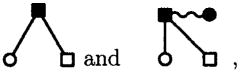
where l_i is the intramolecular bond vector between the sites of molecule i, and u_αγ(r) is the potential between site α on molecule 1 and site γ on molecule 2. Throughout this work on diatomics, our labeling of r and l is an assumed reduction of Chandler's labeling convention,⁷ r_αγ=r_1α2γ and l_i=l_iαiγ, respectively, where r_1α2γ is the vector displacement between site α on molecule 1 and site γ on molecule 2, while l_iαiγ is the vector displacement between sites α and γ, both on molecule i. As used here, then, the site label pairs αα, αγ, γγ as occur in, e.g., Eq. (3) always refer to distinct site pairs on different molecules, and α ≠ γ throughout. We use this reduction for notational convenience only, a more general discussion will require the full notation. This labeling is graphically represented as

(4)

where the wiggly lines represent the intramolecular bond vectors, the squares and circles represent different atomic species, and the dashed lines represent the intermolecular site-site interactions of Eq. (3). The vector expressions of Eqs. (3) and (4) are easily written in the angular coordinates of the two molecules as

$$\begin{array}{l}U({\mathbf{\text{r}}}_{\alpha \gamma },{\mathrm{\Omega }}_1,{\mathrm{\Omega }}_2)=u_{\alpha \gamma }(r_{\alpha \gamma })+u_{\gamma \gamma }({\mathbf{\text{r}}}_{\alpha \gamma },{\mathrm{\Omega }}_1)+u_{\alpha \alpha }({\mathbf{\text{r}}}_{\alpha \gamma },{\mathrm{\Omega }}_2)\hfill \\ +u_{\gamma \alpha }({\mathbf{\text{r}}}_{\alpha \gamma },{\mathrm{\Omega }}_1,{\mathrm{\Omega }}_2)\hfill \\ =u^{\text{o}}(r_{\alpha \gamma })+u^l({\mathbf{\text{r}}}_{\alpha \gamma },{\mathrm{\Omega }}_1)+u^r({\mathbf{\text{r}}}_{\alpha \gamma },{\mathrm{\Omega }}_2)\hfill \\ +u^b({\mathbf{\text{r}}}_{\alpha \gamma },{\mathrm{\Omega }}_1,{\mathrm{\Omega }}_2),\hfill \end{array}$$ (5)

where in the second line we make the natural notational correspondence of the o, l, r, b labeling of Chandler, Silbey, and Ladanyi¹² (CSL) to here indicate that o or none means that there is no angular dependence, l or left means that the term is dependent on the orientation of the left, or “1,” molecule, r or right means that the term is dependent on the orientation of the right, or “2,” molecule, and b or both means that the term is dependent on the orientation of both molecules.

Given this separation of the potential terms, we expand the distribution functions. The closure becomes

$$\begin{array}{c}{c}^o(r_{\alpha \gamma })=e^{-\beta u^o(r_{\alpha \gamma })+t^o(r_{\alpha \gamma })+d^o(r_{\alpha \gamma })}-t^o(r_{\alpha \gamma })-1,\hfill \\ c^l({\mathbf{\text{r}}}_{\alpha \gamma },{\mathrm{\Omega }}_1)=e^{-\beta u^o(r_{\alpha \gamma })+t^o(r_{\alpha \gamma })+d^o(r_{\alpha \gamma })}(e^{-\beta u^l({\mathbf{\text{r}}}_{\alpha \gamma },{\mathrm{\Omega }}_1)+t^l({\mathbf{\text{r}}}_{\alpha \gamma },{\mathrm{\Omega }}_1)+d^l({\mathbf{\text{r}}}_{\alpha \gamma },{\mathrm{\Omega }}_1)}-1)-t^l({\mathbf{\text{r}}}_{\alpha \gamma },{\mathrm{\Omega }}_1),\hfill \\ c^r({\mathbf{\text{r}}}_{\alpha \gamma },{\mathrm{\Omega }}_2)=e^{-\beta u^o(r_{\alpha \gamma })+t^o(r_{\alpha \gamma })+d^o(r_{\alpha \gamma })}(e^{-\beta u^r({\mathbf{\text{r}}}_{\alpha \gamma },{\mathrm{\Omega }}_2)+t^r({\mathbf{\text{r}}}_{\alpha \gamma },{\mathrm{\Omega }}_2)+d^r({\mathbf{\text{r}}}_{\alpha \gamma },{\mathrm{\Omega }}_2)}-1)-t^r({\mathbf{\text{r}}}_{\alpha \gamma },{\mathrm{\Omega }}_2),\hfill \\ c^b({\mathbf{\text{r}}}_{\alpha \gamma },{\mathrm{\Omega }}_1,{\mathrm{\Omega }}_2)=e^{-\beta u^o(r_{\alpha \gamma })+t^o(r_{\alpha \gamma })+d^o(r_{\alpha \gamma })}(\text{exp}[-\beta u^b({\mathbf{\text{r}}}_{\alpha \gamma },{\mathrm{\Omega }}_1,{\mathrm{\Omega }}_2)+t^b({\mathbf{\text{r}}}_{\alpha \gamma },{\mathrm{\Omega }}_1,{\mathrm{\Omega }}_2)+d^b({\mathbf{\text{r}}}_{\alpha \gamma },{\mathrm{\Omega }}_1,{\mathrm{\Omega }}_2)-\beta u^l({\mathbf{\text{r}}}_{\alpha \gamma },\mathrm{\Omega }-1)\hfill \\ +t^l({\mathbf{\text{r}}}_{\alpha \gamma },{\mathrm{\Omega }}_1)+d^l({\mathbf{\text{r}}}_{\alpha \gamma },{\mathrm{\Omega }}_1)-\beta u^r({\mathbf{\text{r}}}_{\alpha \gamma },{\mathrm{\Omega }}_2)+t^r({\mathbf{\text{r}}}_{\alpha \gamma },{\mathrm{\Omega }}_2)+d^r({\mathbf{\text{r}}}_{\alpha \gamma },{\mathrm{\Omega }}_2)]-e^{-\beta u^l({\mathbf{\text{r}}}_{\alpha \gamma },{\mathrm{\Omega }}_1)+t^l({\mathbf{\text{r}}}_{\alpha \gamma },{\mathrm{\Omega }}_1)+d^l({\mathbf{\text{r}}}_{\alpha \gamma },{\mathrm{\Omega }}_1)}\hfill \\ -e^{-\beta u^r({\mathbf{\text{r}}}_{\alpha \gamma },{\mathrm{\Omega }}_2)+t^r({\mathbf{\text{r}}}_{\alpha \gamma },{\mathrm{\Omega }}_2)+d^r({\mathbf{\text{r}}}_{\alpha \gamma },{\mathrm{\Omega }}_2)}+1)-t^b({\mathbf{\text{r}}}_{\alpha \gamma },{\mathrm{\Omega }}_1,{\mathrm{\Omega }}_2).\hfill \end{array}$$ (6)

Since this expansion is still expressed in terms of the full orientation-dependent molecular coordinate system, these are molecularly proper equations in the sense of the CSL theory. As we show below, as long as care is taken to properly account for certain subsets of diagrams through diagrammatic resummation or renormalization, a subset of exponential terms can be properly constructed for each radial site-site function.

The molecular OZ equation (1) expands in the various site-site origin labels as a site-site labeled block matrix, such that the submatrices h_αγ and c_αγ are defined as

$$\begin{array}{l}{\mathbf{\text{h}}}_{\alpha \gamma }=\left(\begin{array}{cc}\begin{array}{c}{h}^o(k_{\alpha \gamma })\\ h^l({\mathbf{\text{k}}}_{\alpha \gamma },{\mathrm{\Omega }}_1)\end{array}& \begin{array}{c}{h}^r({\mathbf{\text{k}}}_{\alpha \gamma },{\mathrm{\Omega }}_2)\\ h^b({\mathbf{\text{k}}}_{\alpha \gamma },{\mathrm{\Omega }}_1,{\mathrm{\Omega }}_2)\end{array}\end{array}\right),\\ {\mathbf{\text{c}}}_{\alpha \gamma }=\left(\begin{array}{cc}\begin{array}{c}{c}^o(k_{\alpha \gamma })\\ c^l({\mathbf{\text{k}}}_{\alpha \gamma },{\mathrm{\Omega }}_1)\end{array}& \begin{array}{c}{c}^r({\mathbf{\text{k}}}_{\alpha \gamma },{\mathrm{\Omega }}_2)\\ c^b({\mathbf{\text{k}}}_{\alpha \gamma },{\mathrm{\Omega }}_1,{\mathrm{\Omega }}_2)\end{array}\end{array}\right),\end{array}$$ (7)

and ρ is now block diagonal, with ρ_αγ=0 in all terms when α ≠ γ and, for this diatomic case,

$${\rho }_{\alpha \alpha }=\left(\begin{array}{cc}\rho /2& \rho /2\\ \rho /2& \rho /2\end{array}\right).$$ (8)

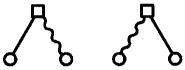
This expansion can be used to diagrammatically resum, or angularly renormalize, the intermolecular distributions in a manner similar to the methods used to treat long-ranged Coulomb potentials in simple fluids.^16,23,24 For example, we consider the expansion of the left molecular diagrams. In the standard diagrammatic notation,^16,25 the left indirect correlation function for a site-site fluid may contain

(9)

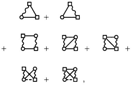
where the solid lines represent site-site Mayer f-bonds, the wiggly bonds represent the rigid, nondissociable intramolecular bonds, circles and squares denote different site species, filled circles and squares represent integrated site position variables, and open circles and squares represent unintegrated site positions. Notice that in this expansion we have not integrated over the 1_γ site or, equivalently, any of the configuration angles of molecule 1. We make the distinction between subsets of diagrams in t^l(r_αγ, Ω₁). which are dependent on only the site in the left molecule labeled 1_γ and those terms which depend on both sites 1_α and 1_γ. We will renormalize the closure by collecting the terms which are exclusively 1_γ dependent in t^l(r_αγ, Ω₁). We note that, by a simple coordinate change, these diagrams are equivalent to the none indirect correlation function between sites 1γ and 2γ, $t_{\gamma \gamma }^o(|{\mathbf{\text{r}}}_{\alpha \gamma }-{\mathbf{\text{l}}}_1|\text{)}$ as determined from the site origin mixture equations, with the γγ labeling here used in the same sense as above for the potential decomposition. Specifically, we change the coordinate system of $t^o(r_{\gamma \gamma })\to t_{\gamma \gamma }^o({\mathbf{\text{r}}}_{\alpha \gamma },{\mathrm{\Omega }}_1)=t_{\gamma \gamma }^o(|{\mathbf{\text{r}}}_{\alpha \gamma }-{\mathbf{\text{l}}}_1|)$ through the coordinate shift r_γγ=r_αγ−l₁. Similarly, t^r(r_αγ, Ω₂) can be renormalized by $t_{\alpha \alpha }^o(|{\mathbf{\text{r}}}_{\alpha \gamma }+{\mathbf{\text{l}}}_2|)$, so that the resummed left and right closure equations, labeled c̄, become

$$\begin{array}{l}{c}^{-l}({\mathbf{\text{r}}}_{\alpha \gamma },{\mathrm{\Omega }}_1)=G^o(r_{\alpha \gamma })[e^{-u^{-l}({\mathbf{\text{r}}}_{\alpha \gamma },{\mathrm{\Omega }}_1)+{\tau }^l({\mathbf{\text{r}}}_{\alpha \gamma },{\mathrm{\Omega }}_1)+d^l({\mathbf{\text{r}}}_{\alpha \gamma },{\mathrm{\Omega }}_1)}-1]\\ -{\tau }^l({\mathbf{\text{r}}}_{\alpha \gamma },{\mathrm{\Omega }}_1),\hfill \\ c^{-r}({\mathbf{\text{r}}}_{\alpha \gamma },{\mathrm{\Omega }}_2)=G^o(r_{\alpha \gamma })[e^{-u^{-r}({\mathbf{\text{r}}}_{\alpha \gamma },{\mathrm{\Omega }}_2)+{\tau }^r({\mathbf{\text{r}}}_{\alpha \gamma },{\mathrm{\Omega }}_2)+d^r({\mathbf{\text{r}}}_{\alpha \gamma },{\mathrm{\Omega }}_2)}-1]\hfill \\ -{\tau }^r({\mathbf{\text{r}}}_{\alpha \gamma },{\mathrm{\Omega }}_2),\hfill \end{array}$$ (10)

which, together with G^o(r_αγ)=exp(−βu^o(r_ay)+t^o(r_αγ) +d^o(r_αγ)), $u^{-l}({\mathbf{\text{r}}}_{\alpha \gamma },{\mathrm{\Omega }}_1)=u^l({\mathbf{\text{r}}}_{\alpha \gamma },{\mathrm{\Omega }}_1)-t_{\gamma \gamma }^o(|{\mathbf{\text{r}}}_{\alpha \gamma }-{\mathbf{\text{l}}}_1|),u^{-r}({\mathbf{\text{r}}}_{\alpha \gamma },{\mathrm{\Omega }}_2)=u^r({\mathbf{\text{r}}}_{\alpha \gamma },{\mathrm{\Omega }}_2)-t_{\alpha \alpha }^o(|{\mathbf{\text{r}}}_{\alpha \gamma }+{\mathbf{\text{l}}}_2|)$, and

$$\begin{array}{l}{\tau }^l({\mathbf{\text{r}}}_{\alpha \gamma },{\mathrm{\Omega }}_1)\equiv t^l({\mathbf{\text{r}}}_{\alpha \gamma },{\mathrm{\Omega }}_1)-t_{\gamma \gamma }^o(|{\mathbf{\text{r}}}_{\alpha \gamma }-{\mathbf{\text{l}}}_1|),\\ {\tau }^r({\mathbf{\text{r}}}_{\alpha \gamma },{\mathrm{\Omega }}_2)\equiv t^r({\mathbf{\text{r}}}_{\alpha \gamma },{\mathrm{\Omega }}_2)-t_{\alpha \alpha }^o(|{\mathbf{\text{r}}}_{\alpha \gamma }+{\mathbf{\text{l}}}_2|),\\ c^l({\mathbf{\text{r}}}_{\alpha \gamma },{\mathrm{\Omega }}_1)=c^{-l}({\mathbf{\text{r}}}_{\alpha \gamma },{\mathrm{\Omega }}_1)-t_{\gamma \gamma }^o(|{\mathbf{\text{r}}}_{\alpha \gamma }-{\mathbf{\text{l}}}_1|)\\ =c^{-l}({\mathbf{\text{r}}}_{\alpha \gamma },{\mathrm{\Omega }}_1)-{\phi }^l({\mathbf{\text{r}}}_{\alpha \gamma },{\mathrm{\Omega }}_1),\hfill \\ c^r({\mathbf{\text{r}}}_{\alpha \gamma },{\mathrm{\Omega }}_2)=c^{-r}({\mathbf{\text{r}}}_{\alpha \gamma },{\mathrm{\Omega }}_2)-t_{\alpha \alpha }^o(|{\mathbf{\text{r}}}_{\alpha \gamma }+{\mathbf{\text{l}}}_2|)\hfill \\ =c^{-r}({\mathbf{\text{r}}}_{\alpha \gamma },{\mathrm{\Omega }}_2)-{\phi }^r({\mathbf{\text{r}}}_{\alpha \gamma },{\mathrm{\Omega }}_2),\hfill \end{array}$$ (11)

give the complete expansion for the c functions and define φ^l(r_αγ, Ω₁) and φ^r(r_αγ, Ω₂). These equations are analogous in form to the short-range form resulting from the renormalization of the Coulomb potential in simple fluid theory.²³ In the “both” case, we similarly use the none, left, and right terms to renormalize the both terms, such that

$$\begin{array}{c}{c}^{-b}({\mathbf{\text{r}}}_{\alpha \gamma },{\mathrm{\Omega }}_1,{\mathrm{\Omega }}_2)=G^o(r_{\alpha \gamma })(\text{exp}[-\beta u^b({\mathbf{\text{r}}}_{\alpha \gamma },{\mathrm{\Omega }}_1,{\mathrm{\Omega }}_2)+t_{\gamma \alpha }^o(|{\mathbf{\text{r}}}_{\alpha \gamma }-{\mathbf{\text{l}}}_1+{\mathbf{\text{l}}}_2|)+{\tau }_{\alpha \alpha }^l({\mathbf{\text{r}}}_{\alpha \gamma }+{\mathbf{\text{l}}}_2,{\mathrm{\Omega }}_1^{\prime })+{\tau }_{\gamma \gamma }^r({\mathbf{\text{r}}}_{\alpha \gamma }-{\mathbf{\text{l}}}_1,{\mathrm{\Omega }}_2^{\prime })+{\tau }^b({\mathbf{\text{r}}}_{\alpha \gamma },{\mathrm{\Omega }}_1,{\mathrm{\Omega }}_2)\hfill \\ +d^b({\mathbf{\text{r}}}_{\alpha \gamma },{\mathrm{\Omega }}_1,{\mathrm{\Omega }}_2)]-G^l({\mathbf{\text{r}}}_{\alpha \gamma },{\mathrm{\Omega }}_1)-G^r({\mathbf{\text{r}}}_{\alpha \gamma },{\mathrm{\Omega }}_2)+1)-{\tau }^b({\mathbf{\text{r}}}_{\alpha \gamma },{\mathrm{\Omega }}_1,{\mathrm{\Omega }}_2)\hfill \\ =G^o(r_{\alpha \gamma })[e^{-u^{-b}({\mathbf{\text{r}}}_{\alpha \gamma },{\mathrm{\Omega }}_1,{\mathrm{\Omega }}_2)+{\tau }^b({\mathbf{\text{r}}}_{\alpha \gamma },{\mathrm{\Omega }}_1,{\mathrm{\Omega }}_2)+d^b({\mathbf{\text{r}}}_{\alpha \gamma },{\mathrm{\Omega }}_1,{\mathrm{\Omega }}_2)}{G}^l{G}^r-G^l({\mathbf{\text{r}}}_{\alpha \gamma },{\mathrm{\Omega }}_1)-G^r({\mathbf{\text{r}}}_{\alpha \gamma },{\mathrm{\Omega }}_2)+1]-{\tau }^b({\mathbf{\text{r}}}_{\alpha \gamma },{\mathrm{\Omega }}_1,{\mathrm{\Omega }}_2),\hfill \end{array}$$ (12)

and

$$\begin{array}{c}{\tau }^b({\mathbf{\text{r}}}_{\alpha \gamma },{\mathrm{\Omega }}_1,{\mathrm{\Omega }}_2)\equiv t^b({\mathbf{\text{r}}}_{\alpha \gamma },{\mathrm{\Omega }}_1,{\mathrm{\Omega }}_2)-{\phi }^b({\mathbf{\text{r}}}_{\alpha \gamma },{\mathrm{\Omega }}_1,{\mathrm{\Omega }}_2),\hfill \\ c^b({\mathbf{\text{r}}}_{\alpha \gamma },{\mathrm{\Omega }}_1,{\mathrm{\Omega }}_2)=c^{-b}({\mathbf{\text{r}}}_{\alpha \gamma },{\mathrm{\Omega }}_1,{\mathrm{\Omega }}_2)-{\phi }^b({\mathbf{\text{r}}}_{\alpha \gamma },{\mathrm{\Omega }}_1,{\mathrm{\Omega }}_2),\hfill \\ {\phi }^b({\mathbf{\text{r}}}_{\alpha \gamma },{\mathrm{\Omega }}_1,{\mathrm{\Omega }}_2),=t_{\gamma \alpha }^o(|{\mathbf{\text{r}}}_{\alpha \gamma }-{\mathbf{\text{l}}}_1+{\mathbf{\text{l}}}_2|)+{\tau }_{\alpha \alpha }^l({\mathbf{\text{r}}}_{\alpha \gamma }+{\mathbf{\text{l}}}_2,{\mathrm{\Omega }}_1^{\prime })\hfill \\ +{\tau }_{\gamma \gamma }^r({\mathbf{\text{r}}}_{\alpha \gamma }-{\mathbf{\text{l}}}_1,{\mathrm{\Omega }}_2^{\prime }),\hfill \\ G^l({\mathbf{\text{r}}}_{\alpha \gamma },{\mathrm{\Omega }}_1)=e^{-u^{-l}({\mathbf{\text{r}}}_{\alpha \gamma },{\mathrm{\Omega }}_1)+{\tau }^l({\mathbf{\text{r}}}_{\alpha \gamma },{\mathrm{\Omega }}_1)+d^l({\mathbf{\text{r}}}_{\alpha \gamma },{\mathrm{\Omega }}_1),}\hfill \\ G^r({\mathbf{\text{r}}}_{\alpha \gamma },{\mathrm{\Omega }}_2)=e^{-u^{-\mathbf{\text{r}}}({\mathbf{\text{r}}}_{\alpha \gamma },{\mathrm{\Omega }}_2)+{\tau }^r({\mathbf{\text{r}}}_{\alpha \gamma },{\mathrm{\Omega }}_2)+d^r({\mathbf{\text{r}}}_{\alpha \gamma },{\mathrm{\Omega }}_2).}\hfill \end{array}$$ (13)

Here, we use ${\mathrm{\Omega }}_i^{\prime }$ as part of the generalized coordinate change, e.g.,

$${\tau }^l({\mathbf{\text{r}}}_{\gamma \alpha },{\mathrm{\Omega }}_1)\to {\tau }_{\gamma \alpha }^l({\mathbf{\text{r}}}_{\alpha \gamma }+\mathbf{\text{l}},{\mathrm{\Omega }}_1^{\prime }),$$ (14)

which is necessary for the statement of the τ^l and τ^r functions in the both coordinate system. The explicit form of the coordinate change will in general be dependent on the particular choice of coordinate representation. The τ¹ and τ^r functions, and not the t^l and t^r functions, are an appropriate choice for resummation in the definition of c^b so as to avoid overcounting many classes of diagrams.

The premise of this approach is succinctly stated in diagrammatic terms. Specifically, we have taken advantage of the equivalence

(15)

where by the operator Lˆ we mean the operation of writing the diagram on the right in the coordinate system on the left by inverting the left bond, which is formally equivalent to changing the coordinate system to coincide with either the circle or square site, respectively. That is, for f₁(r_αγ, Ω₁) the left diagram, f₂(r_γγ) the radially symmetric right diagram before the inversion (equivalently, with the coordinate system coincident with but not rotationally fixed to the square), and l the intramolecular displacement vector between the circle and square sites, we have that

$$f_1({\mathbf{\text{r}}}_{\alpha \gamma },{\mathrm{\Omega }}_1)=f_2(|{\mathbf{\text{r}}}_{\gamma \gamma }-\mathbf{\text{l}}|).$$ (16)

Further, the separation into o, l, r, b terms allows us to renormalize without violating the order of integration, i.e., it maintains the diagrammatically proper construction throughout. Below we show that this renormalization leads directly to the radial PISM equations, and by extension, to an entirely equivalent set of orientation-dependent equations generated from the PISM OZ equations.

B. Low order angular expansion of the site-site equations

Here, we show that the proper site-site integral equation theory is equivalent to a linearized, minimal basis set approximation to the full molecular theory. From the renormalized closure equations above, we linearize with respect to the τ^l, τ^r, and τ^b functions, and expand the l, r, and b e-bonds, i.e., terms such as exp(−ū^l). Ignoring the cross terms and linearizing, we have

$$\begin{array}{l}{h}^o(r_{\alpha \gamma })=e^{-\beta u(r_{\alpha \gamma })+t^o(r_{\alpha \gamma })+d^o(r_{\alpha \gamma })}-1,\hfill \\ h^l({\mathbf{\text{r}}}_{\alpha \gamma },{\mathrm{\Omega }}_1)=G^o(r_{\alpha \gamma })[e^{-u^{-l}({\mathbf{\text{r}}}_{\alpha \gamma },{\mathrm{\Omega }}_1)}-1+{\tau }^l({\mathbf{\text{r}}}_{\alpha \gamma },{\mathrm{\Omega }}_1)\hfill \\ +d^l({\mathbf{\text{r}}}_{\alpha \gamma },{\mathrm{\Omega }}_1)],\hfill \\ h^r({\mathbf{\text{r}}}_{\alpha \gamma },{\mathrm{\Omega }}_2)=G^o(r_{\alpha \gamma })[e^{-u^{-r}({\mathbf{\text{r}}}_{\alpha \gamma },{\mathrm{\Omega }}_2)}-1+{\tau }^r({\mathbf{\text{r}}}_{\alpha \gamma },{\mathrm{\Omega }}_2)\hfill \\ +d^r({\mathbf{\text{r}}}_{\alpha \gamma },{\mathrm{\Omega }}_2)],\hfill \\ h^b({\mathbf{\text{r}}}_{\alpha \gamma },{\mathrm{\Omega }}_1,{\mathrm{\Omega }}_2)=G^o(r_{\alpha \gamma })[e^{-u^{-b}({\mathbf{\text{r}}}_{\alpha \gamma },{\mathrm{\Omega }}_1,{\mathrm{\Omega }}_2)-u^{-l}({\mathbf{\text{r}}}_{\alpha \gamma },{\mathrm{\Omega }}_1)-u^{-r}({\mathbf{\text{r}}}_{\alpha \gamma },{\mathrm{\Omega }}_2)}\hfill \\ +{\tau }^b({\mathbf{\text{r}}}_{\alpha \gamma },{\mathrm{\Omega }}_1,{\mathrm{\Omega }}_2)+d^b({\mathbf{\text{r}}}_{\alpha \gamma },{\mathrm{\Omega }}_1,{\mathrm{\Omega }}_2)\hfill \\ +({\tau }^l({\mathbf{\text{r}}}_{\alpha \gamma },{\mathrm{\Omega }}_1)+d^l({\mathbf{\text{r}}}_{\alpha \gamma },{\mathrm{\Omega }}_1))({\tau }^r({\mathbf{\text{r}}}_{\alpha \gamma },{\mathrm{\Omega }}_2)\hfill \\ +d^r({\mathbf{\text{r}}}_{\alpha \gamma },{\mathrm{\Omega }}_2))-e^{-u^{-l}({\mathbf{\text{r}}}_{\alpha \gamma },{\mathrm{\Omega }}_1)}-e^{-u^{-r}({\mathbf{\text{r}}}_{\alpha \gamma },{\mathrm{\Omega }}_2)}\hfill \\ +1].\hfill \end{array}$$ (17)

Now, in the terminology of Blum and Torruella¹ restricted to linear diatomic molecules, h(r_αγ, Ω₁, Ω₂) may be expanded in rotational invariants Φ^mnl, such that

$$h({\mathbf{\text{r}}}_{\alpha \gamma },{\mathrm{\Omega }}_1,{\mathrm{\Omega }}_2)=\sum _{\mathit{\text{mnl}}}{h}^{\mathit{\text{mnl}}}(r_{\alpha \gamma }){\Phi }^{\mathit{\text{mnl}}}({\mathrm{\Omega }}_1,{\mathrm{\Omega }}_2,R_{\alpha \gamma }),$$ (18)

where the Φ^mnl functions are usually defined in terms of either of two generalized spherical harmonics conventions (Edmonds²⁶ or Messiah²⁷), m, n, l are the indices of the three rotation matrices or rotation angles, R_αγ is the unit vector along the displacement, r_αγ, between molecules in the αγ system, and the h^mnl(r_αγ) are the coefficients of (projections on) the Φ^mnl expansion. If the molecular functions are expanded in this form, then the coefficients in the expansion of h or c may be determined via the molecular OZ equation. In the Edmonds phase and normalization convention¹

$$\begin{array}{l}{h}^{\mathit{\text{mnl}}}(k)-c^{\mathit{\text{mnl}}}(k)=\rho \sum _{n_1{l}_1{l}_2}\frac{(2l+1)}{(2n_1+1)}{(-1)}^{m+n+n_1}\left\{\begin{array}{ccc}{l}_2& l_1& l\\ m& n& n_1\end{array}\right\}\hfill \\ \times \left(\begin{array}{ccc}{l}_1& l_2& l\\ 0& 0& 0\end{array}\right)h^{m{n}_1{l}_1}(k)c^{n_{1}n{l}_2}(k),\hfill \end{array}$$ (19)

where the h^mnl(k) and c^mnl(k) functions are the Hankel transforms of h^mnl(r) and c^mnl(r), respectively, defined as

$$\begin{array}{c}{h}^{\mathit{\text{mnl}}}(k)=4\pi i^l{\int }_0^{\infty }{r}^2{j}_l(kr)h^{\mathit{\text{mnl}}}(r)dr,\\ c^{\mathit{\text{mnl}}}(k)=4\pi i^l{\int }_0^{\infty }{r}^2{j}_l(kr)c^{\mathit{\text{mnl}}}(r)dr,\end{array}$$ (20)

with the j_l(kr) the spherical Bessel functions, the term in parentheses, ( ), in Eq. (19) is the Wigner 3j-symbol,²⁶ and the term in curly braces, { }, is the 6j-symbol. If we now take the minimal, or isotropic, case, h(r_αγ, Ω₁, Ω₂)≈h⁰⁰⁰(r_αγ), then Eq. (19) transformed and expanded in the site coordinate systems reduces to the matrix equation in Fourier space

$$\begin{array}{c}\left(\begin{array}{cc}{\mathbf{\text{h}}}_{\alpha \alpha }\hfill & {\mathbf{\text{h}}}_{\alpha \gamma }\\ {\mathbf{\text{h}}}_{\gamma \alpha }\hfill & {\mathbf{\text{h}}}_{\gamma \gamma }\hfill \end{array}\right)=\left(\begin{array}{cc}{\mathbf{\text{c}}}_{\alpha \alpha }& {\mathbf{\text{c}}}_{\alpha \gamma }\\ {\mathbf{\text{c}}}_{\gamma \alpha }& {\mathbf{\text{c}}}_{\gamma \gamma }\end{array}\right)+\left(\begin{array}{cc}{\mathbf{\text{c}}}_{\alpha \alpha }& {\mathbf{\text{c}}}_{\alpha \gamma }\\ {\mathbf{\text{c}}}_{\gamma \alpha }& {\mathbf{\text{c}}}_{\gamma \gamma }\end{array}\right)\left(\begin{array}{cc}{\mathbf{\rho }}_{\alpha \alpha }& 0\\ 0& {\mathbf{\rho }}_{\gamma \gamma }\end{array}\right)\hfill \\ \times \left(\begin{array}{cc}{\mathbf{\text{h}}}_{\alpha \alpha }& {\mathbf{\text{h}}}_{\alpha \gamma }\\ {\mathbf{\text{h}}}_{\gamma \alpha }& {\mathbf{\text{h}}}_{\gamma \gamma }\end{array}\right),\hfill \end{array}$$ (21)

where the submatrices are defined as

$$\begin{array}{l}{\mathbf{\text{h}}}_{\alpha \gamma }=\left(\begin{array}{cc}{h}^{o,000}(k_{\alpha \gamma })& h^{r,000}(k_{\alpha \gamma })\\ h^{l,000}(k_{\alpha \gamma })& h^{b,000}(k_{\alpha \gamma })\end{array}\right),\\ {\mathbf{\text{c}}}_{\alpha \gamma }=\left(\begin{array}{cc}{c}^{o,000}(k_{\alpha \gamma })& c^{r,000}(k_{\alpha \gamma })\\ c^{l,000}(k_{\alpha \gamma })& c^{b,000}(k_{\alpha \gamma })\end{array}\right),\end{array}$$ (22)

and ρ_αγ=0 if α≠γ,

$${\mathbf{\rho }}_{\alpha \alpha }=\left(\begin{array}{cc}{\rho }^{-o}& {\rho }^{-r}\\ {\rho }^{-l}& {\rho }^{-b}\end{array}\right)=\left(\begin{array}{cc}\rho /2& \rho /2\\ \rho /2& \rho /2\end{array}\right)$$ (23)

otherwise. The closure equations in this approximation can be defined by noting that, as in any basis set expansion, any particular coefficient h^mnl(r_αγ) ∝ ∫dΩ₁dΩ₂h(r_αγ, Ω₁, Ω₂)Φ^mnl, with the proportionality constant given as Ω²=∫dΩ₁dΩ₂(Φ^mnl)². In the minimal basis, this has the convenient form

$$\begin{array}{c}{h}^{000}(r_{\alpha \gamma })={\langle h({\mathbf{\text{r}}}_{\alpha \gamma },{\mathrm{\Omega }}_1,{\mathrm{\Omega }}_2)\rangle }_{{\mathrm{\Omega }}_1{\mathrm{\Omega }}_2}\hfill \\ ={\mathrm{\Omega }}^{-2}\int d{\mathrm{\Omega }}_{1}d{\mathrm{\Omega }}_{2}h({\mathbf{\text{r}}}_{\alpha \gamma },{\mathrm{\Omega }}_1,{\mathrm{\Omega }}_2),\hfill \end{array}$$ (24)

which gives, upon o, l, r, b decomposition, the closure equations

$$\begin{array}{c}{h}^o(r_{\alpha \gamma })=e^{-\beta u^o(r_{\alpha \gamma })+t^o(r_{\alpha \gamma })+d^o(r_{\alpha \gamma })}-1,\hfill \\ h^{l,000}(r_{\alpha \gamma })=G^o(r_{\alpha \gamma })\langle e^{-u^{-l}({\mathbf{\text{r}}}_{\alpha \gamma },{\mathrm{\Omega }}_1)}-1+{\tau }^{l,000}(r_{\alpha \gamma })\hfill \\ +d^l{({\mathbf{\text{r}}}_{\alpha \gamma },{\mathrm{\Omega }}_1)\rangle }_{{\mathrm{\Omega }}_1},\begin{array}{cccc}\begin{array}{cccc}& & & \end{array}\hfill & & \begin{array}{ccc}& & \end{array}& \end{array}\hfill \\ h^{r,000}(r_{\alpha \gamma })=G^o(r_{\alpha \gamma })\langle e^{-u^{-r}({\mathbf{\text{r}}}_{\alpha \gamma },{\mathrm{\Omega }}_2)}-1+{\tau }^{r,000}(r_{\alpha \gamma })\hfill \\ +d^r{({\mathbf{\text{r}}}_{\alpha \gamma },{\mathrm{\Omega }}_2)\rangle }_{{\mathrm{\Omega }}_2},\hfill \\ h^{b,000}(r_{\alpha \gamma })=G^o(r_{\alpha \gamma })[\langle e^{-u^{-b}({\mathbf{\text{r}}}_{\alpha \gamma },{\mathrm{\Omega }}_1,{\mathrm{\Omega }}_2)-u^{-l}({\mathbf{\text{r}}}_{\alpha \gamma },{\mathrm{\Omega }}_1)-u^{-r}({\mathbf{\text{r}}}_{\alpha \gamma },{\mathrm{\Omega }}_2)}\hfill \\ +{\tau }^{b,000}(r_{\alpha \gamma })+d^b({\mathbf{\text{r}}}_{\alpha \gamma },{\mathrm{\Omega }}_1,{\mathrm{\Omega }}_2){\rangle }_{{\mathrm{\Omega }}_1,{\mathrm{\Omega }}_2}\hfill \\ -\langle e^{-u^{-l}({\mathbf{\text{r}}}_{\alpha \gamma },{\mathrm{\Omega }}_1)}\rangle {\mathrm{\Omega }}_1-\langle e^{-u^{-r}({\mathbf{\text{r}}}_{\alpha \gamma },{\mathrm{\Omega }}_2)}\rangle {\mathrm{\Omega }}_2\hfill \\ +({\tau }^{l,000}(r_{\alpha \gamma })+d^{l,000}(r_{\alpha \gamma }))({\tau }^{r,000}(r_{\alpha \gamma })\hfill \\ +d^{r,000}(r_{\alpha \gamma }))+1],\hfill \end{array}$$ (25)

together with the renormalizations

$$\begin{array}{l}{c}^{l,000}(r_{\alpha \gamma })=c^{-l,000}(r_{\alpha \gamma })-{\langle {\phi }^l({\mathbf{\text{r}}}_{\alpha \gamma },{\mathrm{\Omega }}_1)\rangle }_{{\mathrm{\Omega }}_1}\hfill \\ =h^{l,000}(r_{\alpha \gamma })-{\tau }^{l,000}(r_{\alpha \gamma })-{\langle t_{\gamma \gamma }^o(|{\mathbf{\text{r}}}_{\alpha \gamma }-{\mathbf{\text{l}}}_1|)\rangle }_{{\mathrm{\Omega }}_1},\hfill \\ c^{r,000}(r_{\alpha \gamma })=c^{-r,000}(r_{\alpha \gamma })-{\langle {\phi }^r({\mathbf{\text{r}}}_{\alpha \gamma },{\mathrm{\Omega }}_2)\rangle }_{{\mathrm{\Omega }}_2}\hfill \\ =h^{r,000}(r_{\alpha \gamma })-{\tau }^{r,000}(r_{\alpha \gamma })-{\langle t_{\alpha \alpha }^o(|{\mathbf{\text{r}}}_{\alpha \gamma }+{\mathbf{\text{l}}}_2|)\rangle }_{{\mathrm{\Omega }}_2},\hfill \\ c^{b,000}(r_{\alpha \gamma })=c^{-b,000}(r_{\alpha \gamma })-{\langle {\phi }^b({\mathbf{\text{r}}}_{\alpha \gamma },{\mathrm{\Omega }}_1{\mathrm{\Omega }}_2)\rangle }_{{\mathrm{\Omega }}_1,{\mathrm{\Omega }}_2}\hfill \\ =h^{b,000}(r_{\alpha \gamma })-{\tau }^{b,000}(r_{\alpha \gamma })-\langle t_{\gamma \alpha }^o(|{\mathbf{\text{r}}}_{\alpha \gamma }-{\mathbf{\text{l}}}_1+{\mathbf{\text{l}}}_2|)\hfill \\ {+{\tau }_{\alpha \alpha }^{l,000}(|{\mathbf{\text{r}}}_{\alpha \gamma }+{\mathbf{\text{l}}}_2|)+{\tau }_{\gamma \gamma }^{r,000}(|{\mathbf{\text{r}}}_{\alpha \gamma }-{\mathbf{\text{l}}}_1|)\rangle }_{{\mathrm{\Omega }}_1,{\mathrm{\Omega }}_2}.\hfill \end{array}$$ (26)

The forms of φ may be checked against the PISM equations by noting that, by definition, if S_αγ(r)=δ(|r−l|)/(4πl²ρ) is the intramolecular distribution function as normally defined for rigid molecules, then,

$$\begin{array}{l}{x}_{\alpha \gamma }(r)=S_{\alpha \gamma }\ast \rho c_{\gamma \gamma }^o\hfill \\ =\langle e^{-\beta u_{\gamma \gamma }(|{\mathbf{\text{r}}}_{\alpha \gamma }-{\mathbf{\text{l}}}_1|)+t_{\gamma \gamma }^o(|{\mathbf{\text{r}}}_{\alpha \gamma }-{\mathbf{\text{l}}}_1|)}\hfill \\ {-t_{\gamma \gamma }^o(|{\mathbf{\text{r}}}_{\alpha \gamma }-{\mathbf{\text{l}}}_1|)-1\rangle }_{{\mathrm{\Omega }}_1}\hfill \\ ={\langle e^{-\beta u^{-l}({\mathbf{\text{r}}}_{\alpha \gamma },{\mathrm{\Omega }}_1)}-{\phi }^l({\mathbf{\text{r}}}_{\alpha \gamma },{\mathrm{\Omega }}_1)-1\rangle }_{{\mathrm{\Omega }}_1},\hfill \end{array}$$ (27)

where the star denotes the usual convolution product. This, together with similar identities for the other functions, leads to the form derived by Rossky and Chiles for the proper CSL (Ref. 12) OZ equations.

To fully recover the h's in Eq. (25) as the “HNC-like” results of Rossky and Chiles¹³ requires two things. First, we must reform ρ in Eq. (21) such that

$${\mathbf{\rho }}_{\alpha \alpha }=\left(\begin{array}{cc}\rho & \rho \\ \rho & 0\end{array}\right).$$ (28)

This deserves some comment.

First, the elimination of the factor 1/2 in ρ is not ad hoc. In particular, the double counting associated with the split of the original molecular functions of Eq. (1) into site-site coordinates occurs through the ρ^b element alone. Elimination of this element eliminates the doubly counted diagrams which required the 1/2 factor.

To see this, consider the diagram pair,

(29)

which is generated from two different source terms in Eq. (1), i.e., the diagram on the left is generated by the $c^o(r_{ij})\ast {\rho }_{jj}^o{h}^o(r_{jj})$ term, while the diagram on the right, which is obviously equivalent due to the normalization of the molecular S-bond, is generated from the $c^r(r_{ij},{\mathrm{\Omega }}_2)\ast {\rho }_{jj}^b{h}^l(r_{jj},{\mathrm{\Omega }}_1)$ source term in the OZ equations. Note that this particular combination occurs because the diagrams

(30)

are elements of c(r,Ω₁, Ω₂) in the molecular expansion, whereas in the site-site systems, these diagrams are generated in the site-site OZ equations, and necessarily elements of t. Our renormalization assures that these diagrams occur only in φ, not c̄ or τ.

Similar diagram pairs are generated simultaneously in all of the elements of h when the ρ^b elements are included in the OZ matrix, which shows the necessity of the $\frac{1}{2}$ factor in the full ρ matrix. However, by eliminating the ρ^b element, each source term in h becomes unique, and thus the $\frac{1}{2}$ factor is eliminated. This factor will reoccur below, however, when we reintroduce a subset of the source terms contributed via the ρ^b elements; in that case, the $\frac{1}{2}$ factor remains necessary due to doubly counting a certain class of site-site bridge diagrams.

Second, elimination of the ρ^b element together with the linearization of the closure forms a closed set, in that the diagrams which are included may be calculated exactly, i.e., there is no basis set truncation error associated with the diagrams of the minimal angular basis set for those diagrams explicitly included.

Finally, for the HNC-like approximation, the molecular bridge functions must be set to 0, d^o=d^l=d^r=d^b=0, and we must subtract one additional site-site function from h^b,000 [Eq. (25)], such that

$$\begin{array}{c}{h}_{\text{HNC}}^{b,000}(r_{\alpha \gamma })=G^o(r_{\alpha \gamma })[\langle e^{-u^{-b}({\mathbf{\text{r}}}_{\alpha \gamma },{\mathrm{\Omega }}_1,{\mathrm{\Omega }}_2)-u^{-l}({\mathbf{\text{r}}}_{\alpha \gamma },{\mathrm{\Omega }}_1)-u^{-r}({\mathbf{\text{r}}}_{\alpha \gamma },{\mathrm{\Omega }}_2)}\hfill \\ {+{\tau }^{b,000}(r_{\alpha \gamma })+d^b({\mathbf{\text{r}}}_{\alpha \gamma },{\mathrm{\Omega }}_1,{\mathrm{\Omega }}_2)\rangle }_{{\mathrm{\Omega }}_1,{\mathrm{\Omega }}_2}\hfill \\ -\langle (e^{-u^{-b}({\mathbf{\text{r}}}_{\alpha \gamma },{\mathrm{\Omega }}_1,{\mathrm{\Omega }}_2)}-1)(e^{-u^{-l}({\mathbf{\text{r}}}_{\alpha \gamma },{\mathrm{\Omega }}_1)}-1)\hfill \\ {\times (e^{-u^{-r}({\mathbf{\text{r}}}_{\alpha \gamma },{\mathrm{\Omega }}_2)}-1)\rangle }_{{\mathrm{\Omega }}_1,{\mathrm{\Omega }}_2}-{\langle e^{-u^{-l}({\mathbf{\text{r}}}_{\alpha \gamma },{\mathrm{\Omega }}_1)}\rangle }_{{\mathrm{\Omega }}_1}\hfill \\ {-\langle e^{-u^{-r}({\mathbf{\text{r}}}_{\alpha \gamma },{\mathrm{\Omega }}_2)}\rangle }_{{\mathrm{\Omega }}_2}+({\tau }^{l,000}(r_{\alpha \gamma })+d^{l,000}(r_{\alpha \gamma }))\hfill \\ \times ({\tau }^{r,000}(r_{\alpha \gamma })+d^{r,000}(r_{\alpha \gamma }))+1].\hfill \end{array}$$ (31)

For molecules with more than two sites, there would necessarily be similar terms subtracted from h^l,000 and h^r,000, but for diatomics this extension is not necessary.

C. An exact site-renormalized theory for the PISM-OZ equations

The linearization used in generating the diagrammatically proper interaction site formalism directly from the molecular theory is not strictly necessary. Consider Eq. (11). If we truncate at the isotropic basis, we have

$$\begin{array}{l}{h}^{l,000}(r_{\alpha \gamma })=G^o(r_{\alpha \gamma })({\langle e^{-u^{-l}({\mathbf{\text{r}}}_{\alpha \gamma },{\mathrm{\Omega }}_1)+d^l({\mathbf{\text{r}}}_{\alpha \gamma },{\mathrm{\Omega }}_1)+{\tau }^{l,000}(r_{\alpha \gamma })}\rangle }_{{\mathrm{\Omega }}_1}-1)\\ =G^o(r_{\alpha \gamma })({\langle e^{-u^{-l}({\mathbf{\text{r}}}_{\alpha \gamma },{\mathrm{\Omega }}_1)+d^l({\mathbf{\text{r}}}_{\alpha \gamma },{\mathrm{\Omega }}_1)}\rangle }_{{\mathrm{\Omega }}_1}{e}^{{\tau }^{l,000}(r_{\alpha \gamma })}-1).\hfill \end{array}$$ (32)

That is, exp(τ^l,000(r_αγ)) is independent of the angular integrations, by construction, and thus can be factored exactly from the closure statements. We can take advantage of this in the proper formulation by suitably renormalizing the proper OZ site-site matrix equations. In the notation of Rossky and Chiles¹³ together with the modified, screened density approach recently proposed¹⁷, the proper site-site matrix equations in Fourier space are

$$\mathbf{\text{H}}=\mathbf{\text{C}}+\mathbf{\text{C}}\mathbf{\rho }\mathbf{\text{H}},$$ (33)

where

$$\begin{array}{l}{\mathbf{\rho }}_{\alpha \alpha }=\left(\begin{array}{cc}\rho & \eta \\ \eta & 0\end{array}\right),\\ {\mathbf{\text{H}}}_{\alpha \gamma }=\left(\begin{array}{cc}{h}^o(k_{\alpha \gamma })& h^{r,000}(k_{\alpha \gamma })\\ h^{l,000}(k_{\alpha \gamma })& h^{b,000}(k_{\alpha \gamma })+S(k_{\alpha \gamma })\end{array}\right),\\ {\mathbf{\text{C}}}_{\alpha \gamma }=\left(\begin{array}{cc}{c}^o(k_{\alpha \gamma })& c^{r,000}(k_{\alpha \gamma })\\ c^{l,000}(k_{\alpha \gamma })& c^{b,000}(k_{\alpha \gamma })+S(k_{\alpha \gamma })\end{array}\right),\\ S(r_{\alpha \gamma })=\frac{\delta (|r_{\alpha \gamma }-l_{\alpha \gamma }|)}{4\pi l_{\alpha \gamma }^2\eta },\end{array}$$ (34)

l_αγ is the intramolecular bond length, S(r) is the (rigid) intramolecular distribution, and we use η in the general sense, whether as the normalization appropriate to reactive fluids^28–30 or as a bridge function approximation variable.¹⁷ If we now renormalize such that

$$\begin{array}{l}{\mathbf{\tau }}_{\alpha \gamma }={\mathbf{\text{H}}}_{\alpha \gamma }-{\mathbf{\text{C}}}_{\alpha \gamma }-{\mathbf{\phi }}_{\alpha \gamma }={\mathbf{\text{H}}}_{\alpha \gamma }-{\mathbf{\text{C}}}_{\alpha \gamma }\\ =\left(\begin{array}{cc}{t}^o(k_{\alpha \gamma })& {\tau }^{r,000}(k_{\alpha \gamma })\\ {\tau }^{l,000}(k_{\alpha \gamma })& {\tau }^{b,000}(k_{\alpha \gamma }),\end{array}\right),\end{array}$$ (35)

that is, we restrict the functions from the site-site equations to the τ set from Eqs. (11)–(13), then we close the system by

$$\begin{array}{l}{c}^{-o}(r_{\alpha \gamma })=c^o(r_{\alpha \gamma })=e^{-\beta u(r_{\alpha \gamma })+t^o(r_{\alpha \gamma })+d^o(r_{\alpha \gamma })}-t^o(r_{\alpha \gamma })-1,\\ c^{-l,000}(r_{\alpha \gamma })=G^o(r_{\alpha \gamma })({\langle e^{-u^{-l}({\mathbf{\text{r}}}_{\alpha \gamma },{\mathrm{\Omega }}_1)+d^l({\mathbf{\text{r}}}_{\alpha \gamma },{\mathrm{\Omega }}_1)}\rangle }_{{\mathrm{\Omega }}_1}{e}^{{\tau }^{l,000}(r_{\alpha \gamma })}-1)-{\tau }^{l,000}(r_{\alpha \gamma }),\\ c^{-r,000}(r_{\alpha \gamma })=G^o(r_{\alpha \gamma })({\langle e^{-u^{-r}({\mathbf{\text{r}}}_{\alpha \gamma },{\mathrm{\Omega }}_2)+d^r({\mathbf{\text{r}}}_{\alpha \gamma },{\mathrm{\Omega }}_2)}\rangle }_{{\mathrm{\Omega }}_2}{e}^{{\tau }^{r,000}(r_{\alpha \gamma })}-1)-{\tau }^{r,000}(r_{\alpha \gamma }),\\ c^{-b,000}(r_{\alpha \gamma })=G^o(r_{\alpha \gamma })({\langle e^{-u^{-b}({\mathbf{\text{r}}}_{\alpha \gamma },{\mathrm{\Omega }}_1,{\mathrm{\Omega }}_2)-u^{-l}({\mathbf{\text{r}}}_{\alpha \gamma },{\mathrm{\Omega }}_1)-u^{-r}({\mathbf{\text{r}}}_{\alpha \gamma },{\mathrm{\Omega }}_2)+d^b({\mathbf{\text{r}}}_{\alpha \gamma },{\mathrm{\Omega }}_1,{\mathrm{\Omega }}_2)+d^l({\mathbf{\text{r}}}_{\alpha \gamma },{\mathrm{\Omega }}_1)+d^r({\mathbf{\text{r}}}_{\alpha \gamma },{\mathrm{\Omega }}_2)}\rangle }_{{\mathrm{\Omega }}_1,{\mathrm{\Omega }}_2}{e}^{{\tau }^{b,000}(r_{\alpha \gamma })+{\tau }^{l,000}(r_{\alpha \gamma })+{\tau }^{r,000}(r_{\alpha \gamma })}\\ -{\langle e^{-u^{-l}({\mathbf{\text{r}}}_{\alpha \gamma },{\mathrm{\Omega }}_1)+d^l({\mathbf{\text{r}}}_{\alpha \gamma },{\mathrm{\Omega }}_1)}\rangle }_{{\mathrm{\Omega }}_1}{e}^{{\tau }^{l,000}(r_{\alpha \gamma })}-{\langle e^{-u^{-r}({\mathbf{\text{r}}}_{\alpha \gamma },{\mathrm{\Omega }}_2)+d^r({\mathbf{\text{r}}}_{\alpha \gamma },{\mathrm{\Omega }}_2)}\rangle }_{{\mathrm{\Omega }}_2}{e}^{{\tau }^{r,000}(r_{\alpha \gamma })}+1)-{\tau }^{b,000}(r_{\alpha \gamma }),\end{array}$$ (36)

and the renormalization functions are

$$\begin{array}{l}{\phi }^{l,000}(r_{\alpha \gamma })={\langle e^{-u^{-l}({\mathbf{\text{r}}}_{\alpha \gamma },{\mathrm{\Omega }}_1)+d^l(\mathbf{\text{r}},{\mathrm{\Omega }}_1)}\rangle }_{{\mathrm{\Omega }}_1}-1,\\ {\phi }^{r,000}(r_{\alpha \gamma })={\langle e^{-u^{-r}({\mathbf{\text{r}}}_{\alpha \gamma },{\mathrm{\Omega }}_2)+d^r({\mathbf{\text{r}}}_{\alpha \gamma },{\mathrm{\Omega }}_2)}\rangle }_{{\mathrm{\Omega }}_2}-1,\\ {\phi }^{b,000}(r_{\alpha \gamma })={\langle e^{-u^{-b}({\mathbf{\text{r}}}_{\alpha \gamma },{\mathrm{\Omega }}_1,{\mathrm{\Omega }}_2)+d^b({\mathbf{\text{r}}}_{\alpha \gamma },{\mathrm{\Omega }}_1,{\mathrm{\Omega }}_2)-u^{-l}({\mathbf{\text{r}}}_{\alpha \gamma },{\mathrm{\Omega }}_1)+d^l({\mathbf{\text{r}}}_{\alpha \gamma },{\mathrm{\Omega }}_1)-u^{-r}({\mathbf{\text{r}}}_{\alpha \gamma },{\mathrm{\Omega }}_2)+d^r({\mathbf{\text{r}}}_{\alpha \gamma },{\mathrm{\Omega }}_2)}\rangle }_{{\mathrm{\Omega }}_1,{\mathrm{\Omega }}_2}-\langle (e^{-u^{-b}({\mathbf{\text{r}}}_{\alpha \gamma },{\mathrm{\Omega }}_1,{\mathrm{\Omega }}_2)+d^b({\mathbf{\text{r}}}_{\alpha \gamma },{\mathrm{\Omega }}_1,{\mathrm{\Omega }}_2)}-1)\\ \times (e^{-u^{-l}({\mathbf{\text{r}}}_{\alpha \gamma },{\mathrm{\Omega }}_1)+d^l({\mathbf{\text{r}}}_{\alpha \gamma },{\mathrm{\Omega }}_1)}-1){(e^{-u^{-r}({\mathbf{\text{r}}}_{\alpha \gamma },{\mathrm{\Omega }}_2)+d^r({\mathbf{\text{r}}}_{\alpha \gamma },{\mathrm{\Omega }}_2)}-1)\rangle }_{{\mathrm{\Omega }}_1,{\mathrm{\Omega }}_2}-\langle {(e^{-u^{-l}({\mathbf{\text{r}}}_{\alpha \gamma },{\mathrm{\Omega }}_1)+d^l({\mathbf{\text{r}}}_{\alpha \gamma },{\mathrm{\Omega }}_1)-u^{-r}({\mathbf{\text{r}}}_{\alpha \gamma },{\mathrm{\Omega }}_2)+d^r({\mathbf{\text{r}}}_{\alpha \gamma },{\mathrm{\Omega }}_2)})\rangle }_{{\mathrm{\Omega }}_1,{\mathrm{\Omega }}_2}.\end{array}$$ (37)

Though Eqs. (36) and (37) are labeled for the 000 coefficients, the form of these equations does not change for any particular c^mnl(r) coefficient, since the only change then would be to sum over the various terms in τ^mnl in the exponentials rather than truncating at 000, and then take into account the Φ^mnl weighting in the angular average for each coefficient. Therefore, with this labeling caveat, Eqs. (36) and (37) are general and exact for any arbitrary mnl coefficient required. We also note that, by construction, we have, for the HNC approximation truncated at the isotropic basis,

$$\begin{array}{l}g({\mathbf{\text{r}}}_{\alpha \gamma },{\mathrm{\Omega }}_1,{\mathrm{\Omega }}_2)=\text{exp}(-\beta u(r_{\alpha \gamma })+t^o(r_{\alpha \gamma })-u^{-l}({\mathbf{\text{r}}}_{\alpha \gamma },{\mathrm{\Omega }}_1)\\ +{\tau }^{l,000}(r_{\alpha \gamma })-u^{-r}({\mathbf{\text{r}}}_{\alpha \gamma },{\mathrm{\Omega }}_2)+{\tau }^{r,000}(r_{\alpha \gamma })\\ -u^{-b}({\mathbf{\text{r}}}_{\alpha \gamma },{\mathrm{\Omega }}_1,{\mathrm{\Omega }}_2)+{\tau }^b(r_{\alpha \gamma })),\end{array}$$ (38)

that is, we can generate g(r_αγ,Ω₁, Ω₂) self-consistently from the site-site distribution functions through Eqs. (36) and (37). We will use this result below to calculate the diatomic analog of the 3D site-site distribution functions, 〈g(r_αγ,Ω₁,Ω₂)〉_Ω2.

We note that the last two diagrams on h-bonds in the definition of φ^b,000 [the second and third functions of the φ^b,000 definition in Eq. (37)] must be accounted for explicitly, since in the site-site theory the first is a bridge function and necessarily contained in c^−b,000 due to the construction of the OZ matrix, while the l×r multiplication for the second is a c^b diagram in the site-site construction. Further, we only need to restrict the HNC approximation for this closure to the molecular HNC, i.e., d^o=d^l=d^r=d^b=0. Thus, unlike the HNC-like closure of PISM or XRISM, this closure is exact to order ρ⁰, since the intermolecular site-site bridge diagrams of order ρ⁰ are included by construction. Generalization to arbitrary molecules preserves this exactness, since the generalization would be in additional (angular) dimensions, not diagrammatic terms.

Finally, we return the complete isotropic approximation to Eqs. (11)–(13) and (21), and make the system formally exact to order ρ¹, by writing the proper site-site OZ equation as

$$\begin{array}{c}\mathbf{\text{H}}=\mathbf{\chi }+\mathbf{\text{S}}+(\mathbf{\chi }+\mathbf{\text{S}})\mathbf{\rho }\mathbf{\text{H}},\hfill \\ \mathbf{\tau }={[\mathbf{\text{I}}-(\mathbf{\chi }+\mathbf{\text{S}})\mathbf{\rho }]}^{-1}(\mathbf{\chi }+\mathbf{\text{S}})-\overline{\text{c}}-\mathbf{\text{S}},\end{array}$$ (39)

where χ is the proper chain sum²⁰ defined by

$$\mathbf{\chi }={[\mathbf{\text{I}}-\mathbf{\text{c}}{\mathbf{\rho }}^{\prime }]}^{-1}\mathbf{\text{c}},$$ (40)

ρ is the same as Eq. (34), C = c+S=c̄−φ+S, the components of c̄ are the Fourier transforms of Eq. (36), the φ are the Fourier transforms of the functions defined in Eq. (37) (and φ^o,000=0), and ρ′ is defined in general as ${\mathbf{\rho }}_{ij}^{\prime }=0$ when i≠j and

$${\mathbf{\rho }}_{ii}^{\prime }=\left(\begin{array}{cc}0& 0\\ 0& \eta /2\end{array}\right)$$ (41)

otherwise.

That χ is diagrammatically proper, and that the $\frac{1}{2}$ factor in ρ′ is necessary, is easily demonstrated. Consider first the convolution of two angular-dependent molecular f-bonds in the same conventions as Eq. (19),

$$\begin{array}{c}{\langle f({\mathbf{\text{k}}}_{13},{\mathrm{\Omega }}_1,{\mathrm{\Omega }}_3)\rho f({\mathbf{\text{k}}}_{23},{\mathrm{\Omega }}_2,{\mathrm{\Omega }}_3)\rangle }_{{\mathrm{\Omega }}_3}=\sum _{n_1{l}_1{l}_2}\frac{2l+1}{2n_1+1}\\ \times {(-)}^{m+n+n_1}\left\{\begin{array}{ccc}{l}_2& l_1& l\\ m& n& n_1\end{array}\right\}\left(\begin{array}{ccc}{l}_1& l_2& l\\ 0& 0& 0\end{array}\right)\hfill \\ \times f^{m{n}_1{l}_1}(k)\rho f^{n_{1}n{l}_2}(k){\mathbf{\Phi }}^{\text{mnl}}.\hfill \end{array}$$ (42)

If we now expand the molecular f-bonds in site-site potentials, then the site-site diagram

(43)

is clearly a site-site diagrammatic element of the set included in Eq. (42). This is a molecular convolution integral for rigid molecules, but if we use only site-site pair functions, this is a site-site bridge diagram. Now, consider the series in Eq. (42) truncated at (m₁, n₁, l₁, l₂)=(0, 0, 0, 0),

$$\begin{array}{c}{\langle f({\mathbf{\text{k}}}_{13},{\mathrm{\Omega }}_1,{\mathrm{\Omega }}_3)\rho f({\mathbf{\text{k}}}_{23},{\mathrm{\Omega }}_2,{\mathrm{\Omega }}_3)\rangle }_{{\mathrm{\Omega }}_3}\hfill \\ \approx (2l+1){(-)}^{m+n}\left\{\begin{array}{ccc}0& 0& l\\ m& n& 0\end{array}\right\}\left(\begin{array}{ccc}0& 0& l\\ 0& 0& 0\end{array}\right)\hfill \\ \times f^{m00}(k)\rho f^{0n0}(k){\mathbf{\Phi }}^{\text{mnl}}=f^{000}(k)\rho f^{000}(k).\hfill \end{array}$$ (44)

That is, the convolution product diagram

(45)

is then necessarily a member of both Eq. (42) and the truncated series in Eq. (44), and is the first term in the molecular convolution series expansion of the bridge diagram in Eq. (43). Again, as with the exponentiation in the closure, some convolution diagrams which are apparently improper are, in fact, required and a simple consequence of the topological expansion when the generalization to complete angular dependence is accounted for in a full molecular expansion.

Finally, the $\frac{1}{2}$ factor is reintroduced for ρ′ only, due to the symmetry of the S-bond between field points in Eq. (43). Since the site-renormalized series expansions of c^l(r_ij,Ω₁), c^r(r_ij,Ω₂), and c^b(r_ij,Ω₁,Ω₂) from the angular generalizations of Eqs. (36) and (37) collectively begin with the diagram series

(46)

respectively, the class of diagrams which can only be introduced by chaining S-bonds is generated only through Eq. (39), ensuring that each source term in Eqs. (39) and (40) generates a unique, different set of diagrams. However, the χ source equation reintroduces the site-site bridge diagrams, such as Eq. (43), which have S-bonds attached across field points and are generated by the molecular convolution integral. If we were using only one unique coordinate system, then only one of, for instance, the two diagrams such as

(47)

would be generated from the χ equation. Thus, since the χ equation generates all of the possible site-site pair functions simultaneously, and thus generates n equivalent pairs of these bridge diagrams, the 1/n factor, 1/2 here for diatomics, remains for the χ series alone.

In general, χ(r,Ω₁,Ω₂) componentwise in the Φ^mnl expansions is given by

$$\begin{array}{c}{\mathbf{\chi }}^{\mathit{\text{mnl}}}(k)={\mathbf{\text{c}}}^{\mathit{\text{mnl}}}(k)+\sum _{n_1{l}_1{l}_2}\frac{2l+1}{2n_1+1}{(-)}^{m+n+n_1}\left\{\begin{array}{ccc}{l}_2& l_1& l\\ m& n& n_1\end{array}\right\}\\ \times \left(\begin{array}{ccc}{l}_1& l_2& l\\ 0& 0& 0\end{array}\right){\mathbf{\text{c}}}^{m{n}_1{l}_1}{\mathbf{\rho }}^{\prime }{\mathbf{\chi }}^{n_{1}n{l}_2}.\hfill \end{array}$$ (48)

Equation (48) is generated from c, not C, to avoid indiscriminately chaining S-bonds together, which would generate truly improper topological inconsistencies, as in the RISM theory, while still including those (fully connected site-site) molecular diagrams not generated directly by Eq. (39). In the site-site theory, then, χ is another necessary bridge diagram series, and in general, using the expansions of Eq. (48), the proper site-site renormalized OZ equation (39), and the complete Φ^mnl expansions for Eqs. (36) and (37), forms a proper site-site orientation-dependent molecular fluid integral equation theory formally equivalent to the molecular OZ theory of Blum and Torruella. It is thus formally exact, yet embeds the form of the PISM radial site-site theory.

This makes clear the difference in consequences of a derivable mathematical cluster theory for molecular fluids versus augmenting theories with physical cluster rules.¹² Notice above that those diagrams which involve the indiscriminant chaining of S with itself are still disallowed. Yet, there remain classes of diagrams which are consistent with the exponentiation and convolution of the rotational invariants that though they would at first appear to be topologically inconsistent (e.g., RISM) are allowed and required once we make the complete generalization to full molecular rotational dimensionality. These real-space and convolution products contribute to the isotropic correlations even though each diagrammatic term may individually be anisotropic.

III. Results

Here, we present numerical results in the first, isotropic approximation to the theory outlined above. We have calculated the radial distribution functions in the molecular HNC approximation according to Eqs. (36), (37), (39), and (40) for three homonuclear Lennard-Jones diatomic models. For two of the models, l*=l/σ=0.729, 0.547, we have used η=ρ. In the smallest bond length considered here, l*=0.329, which case is a notoriously difficult test of theory, we were unable to obtain a stable solution with η=ρ, and thus took the approximation η≈ρ/(1+(ρπd⁴/3l))=ρ/2.668 from our effective density treatment of homonuclear diatomics.¹⁷ However, following the principle that a solution with η as close to ρ as possible is the best test of the theory as presented, by successive iteration, we were able to effectively minimize the difference between η and ρ and calculate a solution with η=ρ/1.24. We report both results below. Also, for an apolar Lennard-Jones model of HCl we used again η=ρ. Since a self-consistent construction for g(r_αγ, Ω₁,Ω₂) is integral to these calculations, we have also calculated the diatomic analog of the 3D site-site distribution functions, 〈g(r_αγ,Ω₁,Ω₂)〉_Ω2. In the first section, we detail some of the numerical considerations necessary for these calculations. In the second section, we show the results for the homonuclear models, including comparisons of the site-site averages to our effective density variant of PISM and as measured from simulation. In the third section, we present results for the apolar HCl model in comparison to RISM, the standard construction of PISM, and simulation.

Since we published the effective density theory, subsequent analysis has found that the solution for η used in that and prior work³¹ was an asymptotic equation. In those cases, we used a hard sphere result η≈ρ/(1+ρπd⁴/3l). Further work shows that this result is a special case of the general solution, valid for l⪡d. However while this result is a special formal case, in the vast majority of bond lengths, it is still remarkably close to the general result which can be obtained by numerical integration.³² This is further demonstrated in the work using the effective density theory in extension to other closure approximations (work in progress).

A. Numerical methods

Though the angular-dependent terms in Eqs. (36) and (37) are topologically similar to the four-point bridge diagrams previously calculated,^18,19,33 the rigid molecule approximation greatly simplifies these terms, so that the angular averages can be readily calculated using direct integration methods. We use the relative coordinate definitions (r_αγ,Ω₁,Ω₂)=(r_αγ,θ₁,θ₂,φ₁₂) throughout. We choose the intermolecular axis, z, aligned along r_αγ, θ₁ and θ₂ the angles of the intramolecular bond vectors l₁ and l₂ with respect to z, and φ₁₂=φ₁−φ₂ the dihedral angle between the two molecules. For the left and right terms we require the integrals

$$\begin{array}{c}{G}^{l,000}(r_{\alpha \gamma })={\langle e^{-u^{-l}({\mathbf{\text{r}}}_{\alpha \gamma },{\mathrm{\Omega }}_1)}\rangle }_{{\mathrm{\Omega }}_1}=\frac{1}{2}{\int }_0^{\pi }\text{sin}{\theta }_{1}d{\theta }_1\hfill \\ \times e^{-\beta u_{\gamma \gamma }(\sqrt{r_{\alpha \gamma }^2+l^2-2r_{\alpha \gamma }l\text{cos}{\theta }_1})+t_{\gamma \gamma }^o(\sqrt{r_{\alpha \gamma }^2+l^2-2r_{\alpha \gamma }l\text{cos}{\theta }_1}),}\hfill \\ G^{r,000}(r_{\alpha \gamma })={\langle e^{-u^{-r}({\mathbf{\text{r}}}_{\alpha \gamma },{\mathrm{\Omega }}_2)}\rangle }_{{\mathrm{\Omega }}_2}=\frac{1}{2}{\int }_0^{\pi }\text{sin}{\theta }_{2}d{\theta }_2\hfill \\ \times e^{-\beta u_{\alpha \alpha }(\sqrt{r_{\alpha \gamma }^2+l^2+2r_{\alpha \gamma }l\text{cos}{\theta }_2})+t_{\alpha \alpha }^o(\sqrt{r_{\alpha \gamma }^2+l^2+2r_{\alpha \gamma }l\text{cos}{\theta }_2}),}\hfill \end{array}$$ (49)

where l is the bond length, u_γγ(|r_αγ−l|) is the potential between sites γ on molecule 1 and γ on molecule 2 written in the αγ coordinate system, and similarly for the $t_{\gamma \gamma }^o$ terms. These integrals were calculated using a trapezoid rule, with 16 points in θ found to be sufficient for numerical convergence in the cases investigated here. For the both terms, we require

$$\begin{array}{ll}{G}^{b,000}(r_{\alpha \gamma })\hfill & ={\langle e^{-u^{-b}({\mathbf{\text{r}}}_{\alpha \gamma },{\mathrm{\Omega }}_1,{\mathrm{\Omega }}_2)-u^{-l}({\text{r}}_{\alpha \gamma },{\mathrm{\Omega }}_2)-u^{-r}(r_{\alpha \gamma },{\mathrm{\Omega }}_2)}\rangle }_{{\mathrm{\Omega }}_1,{\mathrm{\Omega }}_2}\hfill \\ \hfill & =\frac{1}{8\pi }{\int }_0^{\pi }{\int }_0^{\pi }{\int }_0^{2\pi }\text{sin}{\theta }_{1}d{\theta }_1\text{sin}{\theta }_{2}d{\theta }_{2}d{\phi }_{12}\text{exp}(-\beta u_{\gamma \alpha }(\sqrt{r_{\alpha \gamma }^2+2l^2+2r_{\alpha \gamma }l\text{cos}{\theta }_2-2r_{\alpha \gamma }l\text{cos}{\theta }_1-2l^2\text{cos}{\gamma }_{12}})\hfill \\ \hfill & +t_{\gamma \alpha }^o(\sqrt{r_{\alpha \gamma }^2+2l^2+2r_{\alpha \gamma }l\text{cos}{\theta }_2-2r_{\alpha \gamma }l\text{cos}{\theta }_1-2l^2\text{cos}{\gamma }_{12}})+{\tau }_{\alpha \alpha }^{l,000}(\sqrt{r_{\alpha \gamma }^2+l^2+2r_{\alpha \gamma }l\text{cos}{\theta }_2})\hfill \\ \hfill & +{\tau }_{\gamma \gamma }^{r,000}(\sqrt{r_{\alpha \gamma }^2+l^2-2r_{\alpha \gamma }l\text{cos}{\theta }_1})-\beta u_{\gamma \gamma }(\sqrt{r_{\alpha \gamma }^2+l^2-2r_{\alpha \gamma }l\text{cos}{\theta }_1})+t_{\gamma \gamma }^0(\sqrt{r_{\alpha \gamma }^2+l^2-2r_{\alpha \gamma }l\text{cos}{\theta }_1})\hfill \\ \hfill & -\beta u_{\alpha \alpha }(\sqrt{r_{\alpha \gamma }^2+l^2+2r_{\alpha \gamma }l\text{cos}{\theta }_2})+t_{\alpha \alpha }^0(\sqrt{r_{\alpha \gamma }^2+l^2+2r_{\alpha \gamma }l\text{cos}{\theta }_2})),\hfill \end{array}$$ (50)

with cos γ₁₂ ≡ cos θ₁ cos θ₂ + sin θ₁ sin θ₂ cos φ₁₂, and the other terms required in c^b and the φ^b definitions have similar expansions. For the models examined here, we found sufficient convergence with 16 points in θ and 32 points in φ. The two-dimensional (2D) functions,

$${\langle g({\mathbf{\text{r}}}_{\alpha \gamma },{\mathrm{\Omega }}_1,{\mathrm{\Omega }}_2)\rangle }_{{\mathrm{\Omega }}_2}=g(r_{\alpha \gamma },{\theta }_1)=\frac{1}{4\pi }{\int d{\theta }_{2}d{\phi }_{12}g(r_{\alpha \gamma },{\theta }_1,{\theta }_2,\phi }_{12}),$$ (51)

where g(r_αγ, θ₁, θ₂, φ₁₂) is taken from Eq. (38) in relative coordinates, are a straightforward extension of these integration types, and require only accumulation at the appropriate integration step in the full 3D integrals for the both functions. We also calculate the excess internal energy directly in the usual molecular method from g(r_αγ,θ₁,θ₂,φ₁₂),

$$\begin{array}{ll}\frac{\beta U^{\text{ex}}}{N}\hfill & =2\pi \rho \int r_{\alpha \gamma }^{2}d{r}_{\alpha \gamma }{\langle \beta U({\mathbf{\text{r}}}_{\alpha \gamma },{\mathrm{\Omega }}_1,{\mathrm{\Omega }}_2)g({\mathbf{\text{r}}}_{\alpha \gamma },{\mathrm{\Omega }}_1,{\mathrm{\Omega }}_2)\rangle }_{{\mathrm{\Omega }}_1,{\mathrm{\Omega }}_2}\hfill \\ \hfill & =\frac{1}{4}\rho \int r_{\alpha \gamma }^{2}d{r}_{\alpha \gamma }\text{sin}{\theta }_{1}d{\theta }_1\text{sin}{\theta }_{2}d{\theta }_{2}d{\phi }_{12}(\beta u(r_{\alpha \gamma })+\beta u_{\gamma \gamma }(\sqrt{r_{\alpha \gamma }^2+l^2-2r_{\alpha \gamma }l\text{cos}{\theta }_1})+\beta u_{\alpha \alpha }(\sqrt{r_{\alpha \gamma }^2+l^2+2r_{\alpha \gamma }l\text{cos}{\theta }_2})\hfill \\ \hfill & +\beta u_{\gamma \alpha }(\sqrt{r_{\alpha \gamma }^2+2l^2+2r_{\alpha \gamma }l\text{cos}{\theta }_2-2r_{\alpha \gamma }l\text{cos}{\theta }_1-2l^2\text{cos}{\gamma }_{12}}))g(r_{\alpha \gamma },{\theta }_1,{\theta }_2,{\phi }_{12}),\hfill \end{array}$$ (52)

rather than through the regular site-site expression. For the homonuclear cases, we previously reported βU^ex/N∊* termwise¹⁷ and continue that practice here, which requires dividing the total energy result by 4∊*, where ∊*=T*⁻¹. For the heteronuclear case, we report the full value, βU^ex/N. In principle, though we do not carry out that analysis here, the pressure could also be calculated in closed form from the full molecular definitions, which has not yet proven satisfactory in the standard site-site methods.

In terms of iteration procedures, we treat this system in the same way as was done for atomic h-bonded bridge diagrams,^18,19 in that the angular-averaged terms are held constant while iterating the closure and OZ equations to convergence, and then the new angular averages computed. In all cases considered here, machine-precision convergence for the equations required approximately 12 such total iterations of the angular-averaged functions. In these particular cases, we found no need to use relaxation techniques on the angular terms, though the standard Picard relaxation-iteration procedure for the OZ-closure cycle was necessary.

B. Homonuclear models

Here, we report the results of our calculations for three homonuclear diatomic systems. In all cases, we use the phase point defined in reduced units as ρ*=ρσ³=0.524 and T*=k_BT/∊=2.20, where σ and ∊ are the usual Lennard-Jones parameters. In the homonuclear cases, we report results using a radial grid of 512 points and a range of 15σ, except for both N₂ results, where a grid of 2048 points over a range of 60σ was employed. The three models are for “N₂” or short bond length, l*=l/σ=0.329, “Cl₂” or medium bond length, l*=0.547, and a long bond length model, l*=0.729. We use the approximation defined previously¹⁷ for η for the N₂ model only, with η=ρ/2.668 and η=ρ/1.24, which last was the effective density closest to η=ρ for which we could calculate stable results through successive iteration. For the two longer bond lengths, we use η=ρ.

The g⁰⁰⁰(r) results are summarized in Fig. 1 for the homonuclear cases. In the first case, the structural results using η=ρ/2.668 are not significantly different than our previous calculations in the work on η for this difficult model geometry and phase point. However, the η=ρ/1.24 results are a significant qualitative and quantitative improvement. For the longer bond lengths, with η=ρ, the results are also an overall improvement over the previous results. These changes contribute to an improvement in the thermodynamic values over those previously reported for the η approximation. This is summarized in Tables I and II. Table I gives the results for the Kirkwood-Buff G integral, G_αγ=4π∫r²dr_{α γ}h⁰⁰⁰(r_{α γ}), and Table II gives the (termwise, ∊* reduced) excess internal energy. In these tables, η-HNC is the η=ρ/2.668 approximation with the HNC-like closure, while the results labeled mHNC are the results of this work using Eqs. (36), (37), (39), and (40), here with the η=ρ/1.24 approximation for N₂ and η=ρ otherwise. The results for both thermodynamic quantities investigated are very encouraging, especially in comparison to the results found using previous theories.

FIG. 1.

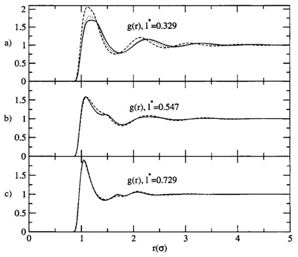
Numerical results for the site-site radial distribution functions for the homonuclear models, the phase points, and model parameters are detailed in the text. r is in units of σ. (a) The l* =0.329 model, the solid line is the simulation result, and the dashed line is the result from this work, with η=ρ/2.668. The dotted line is the result from this work with η=ρ/1.24. (b) The l*=0.547 model, the line types are the same as in (a), with η=ρ here. (c) The l* =0.729 model, the line types are the same as in (a), with η=ρ here.

TABLE I.

Kirkwood-Buff G from simulation and predicted by the various integral equation theories for the homonuclear models in this work.

l*	CSL-HNC	η-HNC	mHNC	Simulation
0.547	−1.77	−1.92	−1.72	−1.79
0.729	−1.78	−2.11	−1.83	−1.88

TABLE II.

Excess internal energy, βU^ex/N∊ per site pair, from simulation and predicted by the various integral equation theories for the homonuclear models.

l*	CSL-HNC	η-HNC	mHNC	Simulation
0.329	…	−3.63	−3.53	−3.50
0.547	−3.52	−3.31	−3.08	−2.99
0.729	−3.05	−2.85	−2.61	−2.64

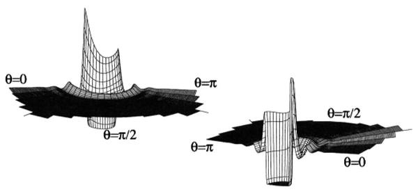
The angular distributions for these models are summarized using two different perspectives in Figs. 2–4 for the short, medium, and long bond lengths, respectively. These are the 2D site-site distribution functions, g(r_αγ, θ₁), calculated self-consistently according to Eqs. (38) and (51). Here, we note the fundamental asymmetries of the homonuclear diatomic system, with the first solvation shell being maximal close to θ₁=π/2, or the x-like configuration, and gradually minimizing to θ₁=0 and θ₂=π, with θ₁=0 being the most favored secondary orientation for all bond lengths. In these cases, we label the σ distance across the right hand figure in order to give perspective, and show that the solvation peaks at θ₁=0 are pushed out by the bond distance, and thus the first shell is pushed out to σ+l in the θ₁=0 case for each bond length, while the θ₁=π first shell distance is approximately σ for each case. In the second shell, the effect of the bond length is also evident, with the N₂ model being the most asymmetric, and the region θ₁=π/2 → θ₁=0 somewhat favored, while in the medium and long bond lengths the secondary solvation shell echoes the first solvation shell of the long bond length, with θ₁=π/2 the most favored orientation, and the θ₁=π,0 orientations symmetrically the secondary orientations. Another interesting feature is the θ₁=π/4 → 0 region in the first solvation shell. Comparing the different bond lengths, it appears that a secondary orientation effect of the first solvation shell towards θ₁=0 is present for all three bond lengths, so that an almost united-atom type “shared” solvation can occur between sites 1 and 2 on molecule 1 for the short and medium bond length models.

FIG. 2.

Two different perspectives of the 2D site-site distribution function g (r_N–N, θ₁) for the N₂ model. The ragged edges are an artifact of the plotting procedure and are not representative of the functions themselves. This is a right-handed coordinate system, with three values for θ=0,π/2, π marked on the plot for orientational convenience. In this figure and Figs. 4 and 5, σ, the contact distance, is labeled along the x axis for perspective.

FIG. 4.

Two different perspectives of the 2D site-site distribution function g(r_αα, θ₁) for the l*=0.729 model.

C. A heteronuclear model

Next, we consider the results for an apolar, heteronuclear model of HCl.³⁴ The presence of an essentially auxiliary site for the H atom makes this model especially interesting. The phase point we use here is ρ=0.018 molecules/ų and T=610 K. We use the standard Lorentz-Berthelot mixing rules, ${∊}_{\mathit{\text{ij}}}=\sqrt{{∊}_{\mathit{\text{ii}}}{∊}_{\mathit{\text{jj}}}}$ and ${\sigma }_{\mathit{\text{ii}}}=\frac{1}{2}({\sigma }_{\mathit{\text{ii}}}+{\sigma }_{\mathit{\text{jj}}})$. The model parameters we use here are a bond length of l=1.3 Å, σ_Cl=3.353 Å, ∊_Cl/k_B=259 K, σ_H=0.4 Å, and ∊_H/k_B=20 K. Strictly speaking, since we are using a complete potential description, the parameters for H are unnecessary in this apolar model. However, RISM and PISM both require an explicit potential for H to avoid collapse at the origin. So, as is a standard practice in integral equation theories, for both simulation and the integral equations, we include the H–H interactions. For emphasis and completeness, we also report results using the theory derived in this work for the HCl model with the H interaction set to 0. The thermodynamic and one-dimensional g(r) results are indistinguishable between the two different models for the calculations from this work and so are not shown, but the g(r,Ω₁) results are significantly different, and are a graphic illustration of the fact that this is a site-site theory which properly solves the so-called auxiliary site problem.

In calculating results for this model, we use a radial grid of 2048 points and range of 30 Å. For clarity and emphasis, we present the RISM and PISM results in Figs. 5(a)–5(c), and the results using the new closure (here with η=ρ, the standard construction) in Figs. 6(a)–6(c). The failures of the RISM and PISM equations are evident in this system. The g_ij(r) results for the new set of equations show clear, significant improvements in all main features over the standard results, and indeed are all but indistinguishable from the simulation results.

FIG. 5.

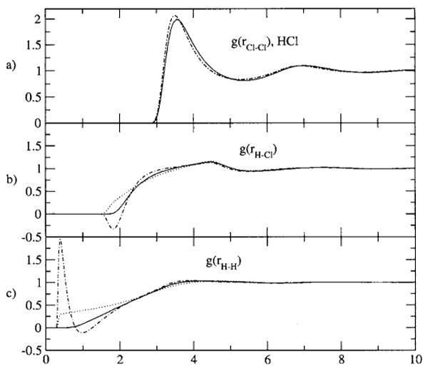
The site-site radial distribution functions as predicted by RISM and standard PISM in comparison to simulation for the HCl model. The model and phase parameters are detailed in the text. r is in angstroms. (a) The Cl-Cl g(r) results, the solid line is simulation, the dotted line is the XRISM result, and the dotted-dashed line is the CSL-HNC result. Here, the XRISM and CSL-HNC results are virtually indistinguishable. (b) The H-Cl g(r) results, the line types are the same as in (a). (c) The H-H g(r) results, the line types are the same as in (a).

FIG. 6.

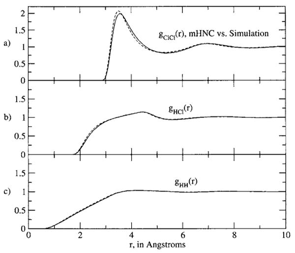
The site-site radial distribution functions predicted by this work for the HCl model. (a) The Cl–Cl g(r) results, with the solid line the simulation result and the dashed line the result of this work, with η=ρ. (b) The H-Cl g(r) results, with the line types the same as in (a). (b) The H–H g(r) results, with the line types the same as in (a). The H–H and H–Cl theory results are essentially indistinguishable from simulation.

The thermodynamic results for this model are summarized in Tables III and IV, where we label CSL-HNC and mHNC as the standard CSL equations with the HNC-like closure and the molecular equations from this work, respectively. For the Kirkwood-Buff G result, we report the results as calculated from the various possible site origins. The results agree to nearly within numerical error across the various site origins, which is a significant and important result as compared to the CSL-HNC equations. In contrast to the homonuclear models, the results for βU/N are essentially equivalent to the CSL-HNC result. It appears to us that the predictions for the thermodynamic quantities for both diagrammatically proper theories are dominated by g_ClCl(r), which is essentially the same in all theories for this particular model. However, these results may prove to be limited by our numerical method, and will be a subject of future investigation.

TABLE III.

Kirkwood-Buff G from simulation and predicted termwise by the various integral equation theories for the apolar HCl model in this work.

G	XRISM	CSL-HNC	mHNC	Simulation
G HH	−43.6	−47.4	−44.7	−48
G HCl	−43.6	−49.9	−44.6	−48
G ClCl	−43.6	−44.3	−44.3	−48

TABLE IV.

Total βU/N from simulation and predicted by the various integral equation theories for the apolar HCl model in this work.

	XRISM	CSL-HNC	mHNC	Simulation
βU/N	−1.69	−1.73	−1.74	−1.69

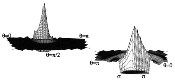
The angular dependence for this model is summarized in Fig. 7, in which we plot g(r_Cl–Cl, θ₁). Unlike the homonuclear cases, this model, as expected from the model parameters, is almost completely symmetric, with only the first solvation shell exhibiting any significant asymmetry. We should also point out that the location of the first solvation shell maximum at θ₁=0, not π/2 as in the homonuclear cases, is consistent with there being little to no direct angular correlation for this model. The inclusion of a H potential in this system is enough to emphasize this dipolelike orientation in the potential, but the H interaction is so small that the intricately detailed effects noted for the angular correlations in the homonuclear cases are not indicated here. A graphic contrast to this model is presented by setting the H potential interaction to 0, which is shown in Fig. 8. For confirmation that this resulting auxiliary site was properly accounted for in the theory, we also calculated the result of changing the bond length as well as zeroing the H potential, and, as expected, the g_ClCl(r, θ₁) results for any bond length investigated were completely identical.

FIG. 7.

Two different perspectives of the 2D Cl–Cl site-site distribution function, g(r_Cl–Cl, θ₁), for the HCl model.

FIG. 8.

Two different perspectives of the 2D Cl–Cl site-site distribution function, g(r_Cl–Cl, θ₁), for the modified HCl model with the H–H interaction parameters set to 0.

This figure demonstrates two things. First, because the H potential is nonexistent, the results for this model are a graphic illustration of the fact that this theory is molecularly complete, and thus does not suffer the so-called auxiliary-site problem, in stark contrast to the RISM and PISM theories. By molecularly complete, we mean that each site-site function in the theory contains the same diagrammatic series, diagrammatically exact to order ρ¹, though each such series is written in a different coordinate system. This is not the case for the RISM and PISM cases, and is the primary reason for the auxiliary site problem in each, as well as the reason that the Kirkwood-Buff G functions are not equivalent in the PISM theory. Furthermore, the generating function of the theory used here is the full molecular f-bond, and thus any expansion element of c which includes the phantom H–H or H–Cl interaction for this model is simply 0, by construction, and thus trivially propagated by the OZ equations. Second, this figure shows that, while the g(r)'s and some thermodynamic quantities may be unaffected by the presence or absence of a small potential around the H, the angular projections and averages can still be significantly and profoundly affected by that potential. This fact will have significant implications in the growing use of the 3D and higher order correlation functions in the study of site-site molecular fluids.

IV. Conclusions

In this work, we have analyzed the molecular pair distribution function for site-site model potentials. We have extended the diagrammatically proper decomposition of Chandler et al.¹² to full angular generality for diatomic site-site molecules, and have used this decomposition to resum, or renormalize, the molecular functions in terms of the resulting orientation-dependent site-site functions. A significant formal result of this analysis is the explicit derivation of the radial diagrammatically proper interaction site theory as a minimal angular basis set approximation to the orientation-dependent molecular fluid theory. This analysis of the minimal site-renormalized theory was then inverted to derive the complete molecular theory as generated from a generalization of the PISM-OZ equations to the orientation-dependent Blum-Torruella expansions. Another significant formal result was that certain subclasses of diagrams which would otherwise be considered diagrammatically improper are instead properly included when the complete angular dependence of site-site molecular interactions is formally accounted for. Thus, we have derived the exact orientation-dependent PISM-OZ analog of the molecular OZ theory. We calculated the radial and 3D distribution functions using the molecular HNC approximation and the isotropic basis for four simple diatomic models, and found improved results for all of the models examined, and in the heteronuclear case the quantitative structural improvement was particularly significant. In addition, the thermodynamic averages for the heteronuclear model preserved necessary symmetries across the various site-site origin pairs of the model. This is also a significant improvement over the standard PISM equations.

The completeness of this theory with respect to the molecular potential of the model under consideration was demonstrated through considering the so-called auxiliary site problem. In particular, because the theory here includes the full molecular potential, we were able to address the problem of auxiliary sites by turning off the interaction potential of one of the sites in the heteronuclear model investigated. The radially symmetric distribution functions and site-site pair dependent thermodynamic quantities investigated here were left unaffected by this for the theory developed here, but the effect of zeroing out the interaction of one of the sites in the angular distribution functions was significant. These results indicate that, first, as would be expected of a molecularly complete theory, the auxiliary site problem that affects the RISM and PISM theory is solved in this case. Second, the introduction of a small potential to such auxiliary sites in molecular potentials in order to avoid this problem in the application of RISM and PISM equations unavoidably introduces nonphysical behavior into higher order correlations which might be generated by or inferred from these theories. This has strong implications for the continuing development of the 3D generalizations of these theories.

These results suggest that further analytic work in this area will be useful. In particular, it seems clear to us that this analysis should be especially useful upon extension to polar fluids. In addition, though the computational method used here may be somewhat cumbersome, the extension to molecules with arbitrary numbers of sites is straightforward. Combined with the fact that the 3D distribution functions are easy to generate from this theory, the work set forth here should provide both a formal and a numerical path forward in investigating more complex molecules.

FIG. 3.

Two different perspectives of the 2D site-site distribution function g(r_Cl–Cl, θ₁) for the Cl₂ model.

References

- 1.Blum L, Torruella AJ. J Chem Phys. 1971;56:303. [Google Scholar]
- 2.Fries PH, Patey GN. J Chem Phys. 1985;82:429. [Google Scholar]
- 3.Carlevaro CM, Blum L, Vericat F. J Chem Phys. 2003;119:5198. [Google Scholar]
- 4.Fries PH, Richardi J. J Chem Phys. 2000;113:9169. [Google Scholar]
- 5.Yoshida N, Kato S. J Chem Phys. 2000;113:4974. [Google Scholar]
- 6.Andersen HC, Chandler D. J Chem Phys. 1972;57:1918. [Google Scholar]
- 7.Chandler D. In: The Liquid State of Matter: Fluids, Simple and Complex. Montroll EW, Lebowitz JL, editors. North-Holland; Amsterdam: 1982. p. 275. [Google Scholar]
- Cortis CM, Rossky PJ, Friesner RA. J Chem Phys. 1997;107:6400. [Google Scholar]
- 9.Kovalenko A, Hirata F. J Chem Phys. 1999;110:10095. [Google Scholar]
- 10.Beglov D, Roux B. J Chem Phys. 1996;104:8678. [Google Scholar]
- 11.Chandler D, Andersen HC. J Chem Phys. 1972;57:1930. [Google Scholar]
- 12.Chandler D, Silbey R, Ladanyi BM. Mol Phys. 1982;46:1335. [Google Scholar]
- 13.Rossky PJ, Chiles RA. Mol Phys. 1984;51:661. [Google Scholar]
- 14.Høye JS, Stell G. J Chem Phys. 1976;65:18. [Google Scholar]
- 15.Lue L, Blankschtein D. J Chem Phys. 1995;102:4203. [Google Scholar]
- 16.Hansen JP, McDonald IR. Theory of Simple Liquids. 2nd. Academic; London: 1986. [Google Scholar]
- 17.Dyer KM, Perkyns JS, Pettitt BM. J Chem Phys. 2005;123:204512. doi: 10.1063/1.2116987. [DOI] [PMC free article] [PubMed] [Google Scholar]
- 18.Perkyns JS, Dyer KM, Pettitt BM. J Chem Phys. 2002;116:9404. [Google Scholar]
- 19.Dyer KM, Perkyns JS, Pettitt BM. J Chem Phys. 2002;116:9413. [Google Scholar]
- 20.Rossky PJ, Dale WDT. J Chem Phys. 1980;73:2457. [Google Scholar]
- 21.Gray CG, Gubbins KE. Theory of Molecular Fluids. Vol. 1 Clarendon; Oxford: 1984. [Google Scholar]
- 22.Friedman HL. A Course in Statistical Mechanics. Prentice-Hall; Engle-wood Cliffs, NJ: 1985. [Google Scholar]
- 23.Allnatt AR. Mol Phys. 1964;8:533. [Google Scholar]
- 24.Ng KC. J Chem Phys. 1974;61:2680. [Google Scholar]
- 25.Ladanyi BM, Chandler D. J Chem Phys. 1975;62:4308. [Google Scholar]
- 26.Edmonds AR. Angular Momenta in Quantum Mechanics. Princeton University Press; Princeton: 1960. [Google Scholar]
- 27.Messiah A. Quantum Mechanics. Wiley; New York: 1958. [Google Scholar]
- 28.Wertheim MS. J Chem Phys. 1987;87:7323. [Google Scholar]
- 29.Kalyuzhnyi YV, Stell G. Mol Phys. 1993;78:1247. [Google Scholar]
- 30.Stell G. Physica A. 1996;231:1. [Google Scholar]
- 31.Dyer KM, Perkyns JS, Pettitt BM. J Chem Phys. 2005;122:236101. doi: 10.1063/1.1893829. [DOI] [PubMed] [Google Scholar]
- 32.Marucho M, Pettitt BM. J Chem Phys. 2007;126:124107. doi: 10.1063/1.2711205. [DOI] [PMC free article] [PubMed] [Google Scholar]
- 33.Perkyns JS, Pettitt BM. Theor Chem Acc. 1997;96:61. [Google Scholar]
- 34.Hirata F, Pettitt BM, Rossky PJ. J Chem Phys. 1982;77:509. [Google Scholar]