A Graphical User Interface for BIOEQS: A Program for Simulating and Analyzing Complex Bio-molecular Interactions

Abstract

BIOEQS is a global analysis and simulations program for complex biomolecular interaction data developed in the 1990’s [1, 2]. Its continued usefulness derives from the fact that it is based on a numerical solver for complex coupled biological equilibria, rather than on closed-form analytical equations for the binding isotherms. It is therefore quite versatile, allowing easy testing of multiple binding models and analysis of systems too complex for closed form solutions. However, a major drawback to a generalized use of this program has been the lack of a graphical user interface (GUI) for setting up the binding models and experimental conditions, as well as visualizing the results. We present here a new GUI for BIOEQS that should be useful in both research and teaching applications.

Simulation and analysis of complex biomolecular binding equilibria are key elements to both the design of binding experiments and the interpretation of interaction data. Moreover, these approaches are covered in many graduate and undergraduate courses in biochemistry and biophysics. BIOEQS is a relatively powerful numerically based program designed for the simulation and global analysis of such complex data sets [1, 2]. Rather than solving a closed form analytical expression for the binding isotherm, the BIOEQS solver uses a numerical constrained optimization algorithm, with the mass balance constraints incorporated as Lagrange multipliers, to solve the set of non-linear equations for the free energies of formation of each species, in terms of the species concentration vector. This solver is called at each point of the binding isotherm to calculate the isotherm based on the input free energy and observable asymptotic parameters. To obtain best fit free energy and other parameters, the fitting routine is based on a non-linear Marquardt-Levenberg algorithm. The program was originally conceived to treat a very broad range of binding experiments, in terms of number of elements, number of species, observable parameters and thermodynamic variable (temperature, pressure or chemical potential).

The advantage of the GUI described here resides in the ready accessibility of many of the available options of BIOEQS. These can be modified quickly with the corresponding results examined at a faster pace and with little knowledge of the intricacies of the subroutines. BIOEQS functions using ASCII format I/O files (2 input and 4 output), the structures of which have been preserved for compatibility and for advanced users. However, in the GUI, the user no longer needs to modify these files directly.

We describe here the basic structure of the graphical user interface (GUI) designed for BIOEQS by following the necessary steps from model making to confidence limit interval analysis. Here, we have simulated data for a binding model including six species, a DNA-protein interaction with stoichiometries from one to four proteins. The other two species are the free DNA and the free protein. Then these simulated data were analyzed globally to demonstrate the GUI analysis output.

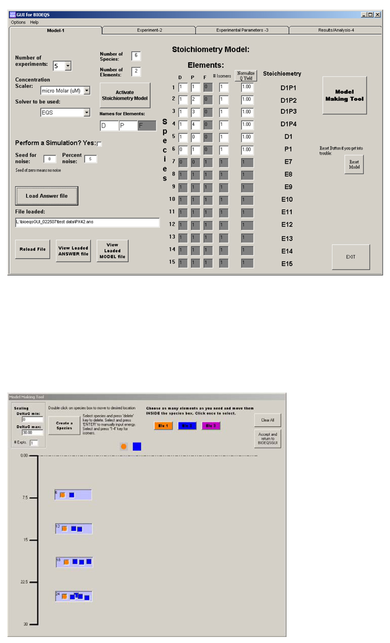
The BIOEQS GUI is divided into four pages or tabs; a model, an experiment, a fitting parameters and a results page. The program initializes in the model page (Figure 1a) where the first step is to create the model containing all the information necessary for composition of each species including stoichiometry and number of site isomers. (A quantum yield factor allows for assignment of unequal weighting of the species in the observable). A model making tool (Figure 1b) allows for creating species by dragging and dropping elements into species boxes that can also be dragged and placed within a specific free energy range. The model can also be built manually. The BIOEQS program has a limit of three different elements and the GUI has a limit of fifteen unique species (100 for the kernel). Drop down menus allow the user to specify the concentration range and the number of experiments (maximum 16). The default solver of the GUI is the numerical one mentioned above, but a closed-form analytical solver for monomeric protein folding can also be specified. If a simulation is performed, a seed for the noise and percent noise become available options.

Figure 1.

a) The Model page is shown with six species (including the identity matrix) with the Model Making Tool in (b) showing the four species containing DNA and protein elements with color coded icons.

The next two pages involve the specification of the experimental and fitting parameters. The available options depend on the type of experiment. For each experiment, the user must specify what type of observable is to be mapped (i.e. total or fractional contribution to the total signal for a particular element, or the population of a specific species) and the actual experiment type performed, i.e. titration, folding, pressure or temperature. Also, depending on the type of the experiment, the concentration for the other elements, the concentration of chemical additive (denaturant, salt, osmolyte), the pressure or the temperature of the experiment may be required. In our example, for all the experiments, we chose a fractional population (with respect to total DNA) for each of the species containing DNA (species 1–5). The experiment type was a titration of the first element (DNA) at 0.1 µM with protein at a temperature of 291 K and at 1 bar. If a simulation is performed, the simulated data files are also created on this page. We created five files starting at 0.1 and ending at 1000 µM with a step of log 0.1 units, each file corresponding to the fractional population of each of the DNA containing species.

The fitting parameters (free energies of formation (from the free elements) for each of the species, asymptotic observable values, and thermodynamic parameters such as m-values, volume changes or enthalpy changes) are found in the Master Table on the Experimental Parameters page (page 3). Because BIOEQS is a global analysis program, the GUI includes algorithms to deduce the appropriate parameter numbering scheme, and thus linking of the different parameters energies across experiments is also done on this table. For our example, the energies were linked across all five experiments and allowed to vary. The initial guesses for the species were 6, 12, 18 and 24 kcal/mol. The asymptotic values of fractional populations were normalized between 0 and 1, but for real experiments they can in fact be any number resulting from an experimental observable.

The BIOEQS FORTRAN 77 code has been re-compiled as a dynamic link library (DLL) that is called directly with all the parameters (There is no longer a need to run the program in a MS-DOS window). The use of a DLL allows for multiple instances and sequential calls to the DLL, as when performing a covariance analysis (see below). The output, including any errors produced by the DLL, are displayed as the calculation progresses in textboxes located next to the Master Table in the Experiment parameters page.

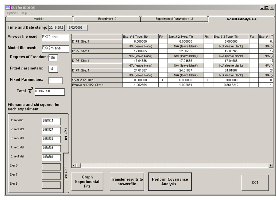
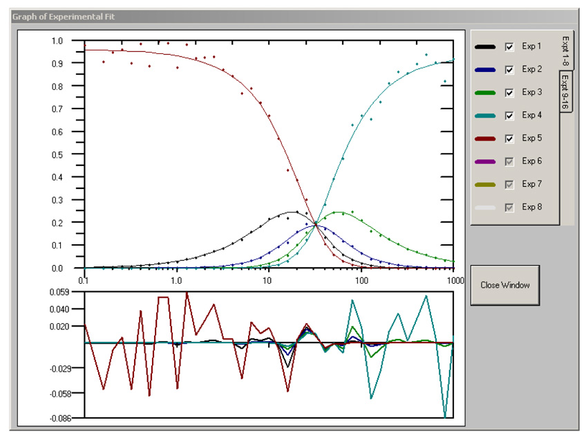
The Results page displays in table format all the returned parameter values for each experiment as well as the local and global χ² values (Figure 2a). Another useful aspect of the BIOEQS GUI is the rapid graphic display of the fit results (Figure 2b), including residuals for all the experiments. The recovered parameter values are stored in an ASCII file with a *.res extension and the initial data, fit and residuals for each experiment are placed in a file with the *.tmp extension.

Figure 2.

a) The Results page with the graphed results with residuals in (b) and the covariance analysis (c) of the first element of experiment #1.

Rigorous confidence limit testing and covariance analysis can be also performed for up to 20 unique parameters over a specified interval in specified steps. The output table includes the covariance of all the parameters for each experiment due to the change of the specified parameter. The calculated χ² for that step is used as a header on each column. Also, a graph of χ² vs parameter (confidence limit) is plotted for each variable including a line at the 67% and 97% interval (Figure 2c). In our example, we chose the first free energy of the first experiment to be rigorously tested between 5.2 to 6.4 kcal/mol with steps of 0.2 kcal/mol. For rapid recognition, the selected variable is shown in purple in the Covariance Table. The results are placed in files with a *.cov and a *.con extension.

Given the broad capabilities of the BIOEQS fitting program, we hope that the development of the GUI will allow the program to be widely used. In particular, it could be a very useful tool in upper level undergraduate or graduate courses that cover biomolecular interactions. The program with the installation package and a brief description of the I/O files can be found at the following link: http://abcis.cbs.cnrs.fr/BIOEQS/.

References

- 1.Royer CA, Smith WR, Beechem JM. Analysis of Binding in Macromolecular Complexes: A Generalized Numerical Approach. Anal. Biochem. 1990;191:287–294. doi: 10.1016/0003-2697(90)90221-t. [DOI] [PubMed] [Google Scholar]
- 2.Royer CA, Beechem JM. Numerical Analysis of Binding Data: Advantages, Practical Aspects and Implications. Methods in Enzymology. 1992;210:481–505. doi: 10.1016/0076-6879(92)10025-9. [DOI] [PubMed] [Google Scholar]