Statistical Segmentation of Surgical Instruments in 3D Ultrasound Images

Abstract

The recent development of real-time 3D ultrasound enables intracardiac beating heart procedures, but the distorted appearance of surgical instruments is a major challenge to surgeons. In addition, tissue and instruments have similar gray levels in US images and the interface between instruments and tissue is poorly defined. We present an algorithm that automatically estimates instrument location in intracardiac procedures. Expert-segmented images are used to initialize the statistical distributions of blood, tissue and instruments. Voxels are labeled through an iterative expectation-maximization algorithm using information from the neighboring voxels through a smoothing kernel. Once the three classes of voxels are separated, additional neighboring information is combined with the known shape characteristics of instruments in order to correct for misclassifications. We analyze the major axis of segmented data through their principal components and refine the results by a watershed transform, which corrects the results at the contact between instrument and tissue. We present results on 3D in-vitro data from a tank trial, and 3D in-vivo data from cardiac interventions on porcine beating hearts, using instruments of four types of materials. The comparison of algorithm results to expert-annotated images shows the correct segmentation and position of the instrument shaft.

INTRODUCTION

The recent development of clinical real-time 3D ultrasound (US) enables new intracardiac beating heart procedures (Cannon et al. 2003; Downing et al. 2002; Shapiro et al. 1998; Suematsu et al. 2005), avoiding the use of cardiopulmonary bypass with its attendant risks. Unfortunately, these images are difficult for the surgeon to interpret, due to poor signal-to-noise ratio and the distorted appearance of surgical instruments within the heart (Cannon et al. 2003). Automated techniques for tracking instrument location and orientation would permit augmentation of intraoperative displays for the surgeon as well as enable image-based robotic instrument control (Stoll et al. 2006).

Image-guided interventions require the simultaneous visualization of instruments and tissue. In US-guided procedures, metallic instruments hamper the already difficult visualization of tissue. Since US is designed to image soft tissue, the strong reflections caused by smooth metal surfaces saturate the image. This places in shadow the structures behind the instrument, while the location and orientation of the instrument remain uncertain. Reverberations and artifacts create more confusion in complex in-vivo images (Figure 1).

Figure 1.

A 2D US image of an instrument of stainless steel coated with tape in a water tank. The appearance of the metal rod is distorted by the presence of reverberations and tip artifacts.

We are working on developing US-guided cardiac procedures for atrial septal defect closures. Our project proposed using rigid instruments through the chest wall, demonstrated in animals. The feasibility of the procedures and their limitations can be found in (Downing et al. 2002; Suematsu et al. 2005). Reliable visualization of structures within the heart remains a major challenge to successful beating-heart surgical interventions and robotic-assisted procedures.

Most work in cardiac imaging relates to heart visualization and diagnosis and not to cardiac interventions. Knowledge-based constraints, similar to a priori shape knowledge, are used to segment cardiac tissue in level set approaches in (Lin et al. 2003; Paragios 2003). A combination of wavelets and deformable models is proposed in (Angelini et al. 2005), active appearance models are exploited in (Mitchell et al. 2002) and Xiao et al. (2002) use tissue texture analysis to segment cardiac images. However, little work has been devoted to correcting the distorted appearance of instruments under ultrasound imaging. Tissue and instruments have similar gray levels in US images, which makes their correct delineation difficult. Shadows, reverberations and tip artifacts can puzzle even the trained eye, and the fuzzy interface between instruments and tissue is confusing to the surgeon (Figure 1).

Researchers have recognized that US imaging of existing instruments is problematic. A variety of techniques have been applied to improve instrument imaging (mostly for needles since US has been 2D until recently). These techniques have included material selection, surface modifications and coatings (Hopkins and Bradley 2001; Nichols et al. 2003; Huang et al. 2006). As 3D US becomes widely available, more complex 3D tasks will be performed under US guidance, such as robotic interventions, and it is recognized that instruments will need to be modified for improved imaging. Obviously, techniques like applying coatings to existing instruments are the most economical, but it is also of value to predict how well alternate materials would perform.

Ortmeier et al. (2005) track instruments for visual servoing in 2D US images. Their experimental setup consists of graspers made of various materials (PVC, nylon, polyurethane) in a water tank. The position and shape of their instruments are known a priori. The head of the grasper is identified using thresholding and morphological operators. Although fast and simple, the method identifies the tips of the instrument in an in-vitro setting without the presence of tissue.

Novotny et al. (2003; Stoll et al. 2006) localize an instrument in a tank setup, but in the presence of tissue. The instrument is identified from its principal component analysis (PCA) as the longest and thinnest structure in the US image. However, the instrument and tissue are not in contact, which would change the geometry of the connected components in the image. Passive markers are placed on the instrument to help with its localization. Ding et al. (2003) segment needles from orthogonal 2D projections for breast and prostate biopsy and therapy applications. They segment needles placed in turkey breast in this fast technique, but need a priori knowledge about the needle direction and entrance points.

Our work includes instruments as well as tissue and blood in an intensity-histogram-based analysis and eliminates false positives (FP) using a priori shape information. The following section describes the methodology of the instrument segmentation, a combination of expectation-maximization (EM), principal component analysis (PCA) and watershed transform (WT) algorithms. Then, we present results on detecting instruments of various materials from tank studies and in-vivo interventions that demonstrate the successful delineation of both the position and orientation of the instrument.

METHODS

The algorithm consists of three major steps to segment surgical instruments in echocardiographic images. First, it estimates from expert-segmented intracardiac images the gray level distributions of blood, tissue and instruments. It then builds averaged probability distribution functions for the three classes and labels image voxels through an iterative EM algorithm. The next step analyzes the major axis of the labeled connected components of the image through their principal components. The results are refined by a watershed transform by immersion, which corrects the errors at the contact between instrument and tissue. Our method for segmentation of 3D US images distinguishes between three classes of voxels: blood, tissue, and instruments. Figure 2 presents a schematic diagram of the algorithm.

Figure 2.

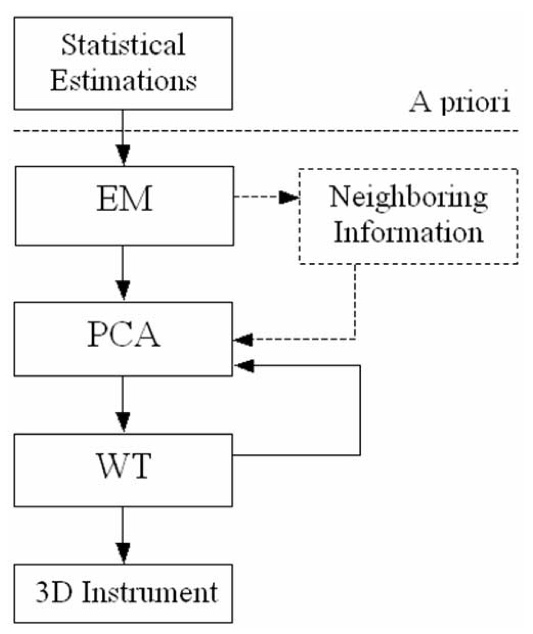
The algorithm for instrument segmentation in 3D ultrasound images. The neighboring information step is optional, as explained in the Results section.

Expectation-maximization

In the expectation-maximization (EM) algorithm (Couvreur 1996), the maximum likelihood parameters are computed iteratively starting with the initial estimation. The algorithm converges to a steady state once a local maximum is reached. At each iteration, there is:

• an expectation step: the unobserved variables are estimated from the observed variables and the current parameters;

• a maximization step: the parameters are re-evaluated to maximize likelihood, assuming that the expectation is correct.

We employ the EM algorithm to solve a mixture estimation problem and separate blood, tissue and instruments. We express the distribution function as a sum of three Gaussians

$$f\left(x\right)={\displaystyle \sum _{n=1}^3{\pi }_n·G\left(x;{\mu }_n;{\sigma }_n\right),}$$ (1)

where the parameters of the Gaussians are

$${\displaystyle \sum _{n=1}^3{\pi }_n=1,{\mu }_n=\frac{1}{N}{\displaystyle \sum _{i=1}^N{x}_i,{\sigma }_n^2=\frac{1}{N}{\displaystyle \sum _{i=1}^N{\left(x_i-{\mu }_n\right)}^2.}}}$$ (2)

The parameters of the three distributions are computed in the expectation step. Let X = (x₁, x₂,…,x_N) be the sequence of observations from the mixture of three Gaussians and θ = {π₁, π₂, π₃, σ₁, σ₂, σ₃, μ₁, μ₂, μ₃} the parameters that must be estimated from X. The values of the parameters π, σ and μ will be updated with each iteration until the algorithm converges. The likelihood maximization then requires maximizing

$$\text{ln}P\left(X|\theta \right)={\displaystyle \sum _{i=1}^N\text{ln}P\left(x_i|\theta \right)}.$$ (3)

In a simplified presentation, the EM algorithm tries to determine the probability of a voxel belonging to one of the three defined classes Γ₁, Γ₂, Γ₃. Using the parameters θ and Bayes’s law we can compute P(x_i∈ Γ_j) as

$$P\left(x_i\in {\mathrm{\Gamma }}_j\right)=\frac{{\pi }_j·G\left(x_i;{\mu }_j;{\sigma }_j\right)}{{\displaystyle \sum _n{\pi }_n·G\left(x_i;{\mu }_n;{\sigma }_n\right)}}.$$ (4)

The maximization step will update the values of the parameters

$${\mu }_j=\frac{{\displaystyle \sum _{i}P\left(x_i\in {\mathrm{\Gamma }}_j\right)·x_i}}{{\displaystyle \sum _{i}P\left(x_i\in {\mathrm{\Gamma }}_j\right)}},{\pi }_j=\frac{{\displaystyle \sum _{i}P\left(x_i\in \mathrm{\Gamma }{}_j\right)}}{{\displaystyle \sum _{i,n}P\left(x_i\in {\mathrm{\Gamma }}_n\right)}},{\sigma }_j^2=\frac{{\displaystyle \sum _{i}P\left(x_i\in {\mathrm{\Gamma }}_j\right)·{\left(x_i-{\mu }_j\right)}^2}}{{\displaystyle \sum _{i}P\left(x_i\in {\mathrm{\Gamma }}_j\right)}}.$$ (5)

The initial estimate of the three classes is extracted from expert-segmented images. This provides the statistical distributions of blood, tissue and instruments, as in Figure 3. Each observation is then approximated from the neighboring voxels through a smoothing kernel. The histograms of the three classes are not fully separated, as seen in Figure 3. The main uncertainty occurs at the overlap between tissue and instrument intensities.

Figure 3.

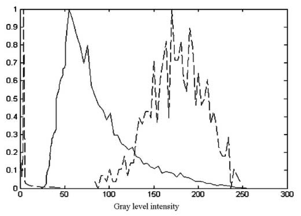
The normalized histograms of blood (dashed-left), tissue (solid-middle) and instrument (dashed-right). The example shows the histogram of a wood instrument. Note the overlap between the tissue and instrument histograms, the main source of uncertainty in the EM algorithm.

As the separation between blood and the other two classes is straightforward, the final goal of the algorithm is to split the uncertainty class between tissue and instrument. Voxels are labeled iteratively until the rate of change between iterations becomes smaller than a given limit. Due to the larger number of tissue voxels in the observation, the maximum likelihood parameters tend to give priority to tissue over instrument, if weights π are equal. For that reason, we gave larger weights to the instrument distribution. Since the percentage of instrument voxels is not known in advance, the weights are set empirically: 1 for blood, 1 for tissue and 3 for instrument. The number of iterations for convergence of the algorithm can vary slightly, and more importantly, the number of voxels correctly classified as instrument is increased.

Neighboring Information

The second stage of the method uses spatial measures based on the shape and size of instruments to correct for misclassified voxels. The assumption imposed here is that instruments are long and thin. We employ three kernels around a central voxel (CV), as seen in Figure 4:

• μ_C : a central kernel (3×3×3), smaller than the size of instruments;

• μ_N : a larger neighboring kernel (7×7×7 excluding the central kernel);

• μ_B : a large background kernel (21×21×21 excluding the neighboring kernel).

Figure 4.

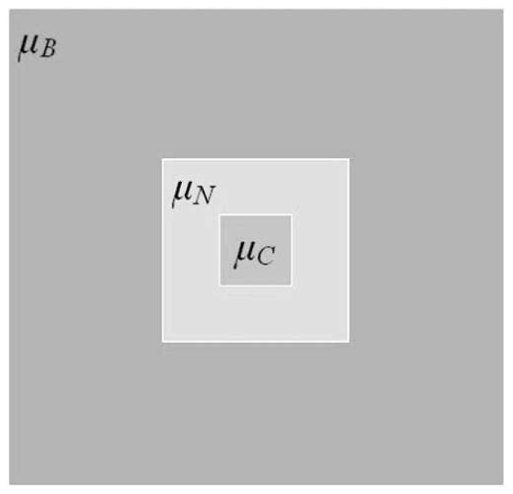
The kernel used for neighboring information. μ_C is the central kernel, μ_N is the neighboring kernel, while μ_B is the background kernel. This is a 2D representation of the 3D kernels.

The relations between the three kernels aim to correct for voxels labeled incorrectly. The kernels are applied to the labeled image, which consist of labels for blood, tissue and instrument. We compute median values for each kernel, to represent the majority of classified voxels. For instance, if μ_C is close to tissue, μ_N to instrument and μ_B to blood, this corresponds to instrument voxels misclassified as tissue on the instrument shaft placed in the blood pool. Based on observations of in vivo images, there are three situations to consider:

• small volumes misclassified as tissue within the instrument shaft or tip (an instrument is more likely to be surrounded by blood)

  IF μ_C ~=tissue AND μ_N ~=instrument AND μ_B ~=blood THEN CV ==instrument;

• small volumes mislabeled as blood within volumes labeled as instrument (there is no blood in instruments and not likely in large tissues)

  IF μ_C ~=blood AND μ_N ~=instrument THEN CV ==instrument;

  IF μ_C ~=blood AND μ_N ~=tissue AND μ_B ~=tissue THEN CV ==tissue.

• small volumes misclassified as instrument within large volumes of tissue (instruments are bigger and not fully covered by tissue)

  IF μ_C ~=instrument AND μ_N ~=tissue AND μ_B ~=tissue THEN CV ==tissue.

This neighboring information step was designed for in vitro data.

Principal Component Analysis

Next, principal component analysis (PCA) (Jackson 1991) is used to detect candidates for the instrument shaft. A practical way to compute principal component is by extracting the eigenvalues from the covariance matrix of the data. Eigenvalues represent the projected variances corresponding to principal components. For a matrix Im, the covariance matrix C_Im is computed as

$$C_{\text{Im}}=\langle \left(\text{Im}-{\mu }_{\text{Im}}\right){\left(\mathrm{Im}-{\mu }_{\mathrm{Im}}\right)}^T\rangle .$$ (6)

In our application, the image is separated in connected components (CC) before performing PCA. Voxels must share at least one corner with their neighbors to be part of the same connected component (3D 26-connected neighborhood). For each CC, we extract the spatial information of its p voxels in a p×3 matrix I_CC for which we compute a 3×3 covariance matrix C_CC. Under the assumption that an instrument is long and thin, its first principal component would account for most of its variation. Hence, if the instrument eigenvalues are calculated as

$$\left|C_{CC}-\lambda I\right|=0;F=\frac{{\lambda }_{CC1}}{{\lambda }_{CC2}},$$ (7)

The first eigenvalue λ_CC1 will be dominant and the ratio F would have a maximal value, where λ_CC2 is the second eigenvalue.

The objects with the highest ratio F are instrument candidates. If there is only one instrument in the image, it will have the maximal F. Due to estimation errors in EM at the contact between instrument and tissue, we prefer to keep more candidates and discard the remaining false positives (FP) in the next stage.

Watershed Transform

To account for errors at the contact between instrument and tissue, we use a watershed (WT) by immersion algorithm (Grau et al. 2004; Roerdinck et al. 2000; Vincent et al. 1991) that assumes that there is only one instrument in every image. WT is a morphological tool that analyses the topography of the image based on its gray level. It presumes that water penetrates minima and floods all areas below the water level to form basins. Eventually basins start merging at watershed lines.

WT is applied to the instrument candidates resulting from the previous PCA and using the estimate of instrument statistics from EM. First, the Euclidean intensity distances to the upper quartile of the instrument intensity are calculated, then a gradient of the newly computed image is used to initialize local minima.

$${\text{Im}}_q=\text{max}\left(\text{Im}\right)-\left|\text{Im}-\left({\mu }_{instr}+{\sigma }_{instr}\right)\right|;{\text{Im}}_g=\left|G_{\sigma }^{\prime }\left({\text{Im}}_q\right)\right|.$$ (8)

The computation of watershed lines is done through two topographic measures: the lower slope (LS) and the lower neighborhood (LN).

$$LS\left(x\in {\text{Im}}_g\right)={\text{max}}_{y\in N_x}\left(\frac{{\text{Im}}_g\left(x\right)-{\text{Im}}_g\left(y\right)}{d\left(x,y\right)}\right);$$ (9)

$$LN\left(x\in {\text{Im}}_g\right)=\left\{y\in N_x|\frac{{\text{Im}}_g\left(x\right)-{\text{Im}}_g\left(y\right)}{d\left(x,y\right)}=LS\left(x\right)\right\};$$ (10)

LS maximizes the relation of voxels y in the neighborhood N_x of voxel x, where d(x,y) is the Euclidian distance between the locations of voxels x and y. LN identifies the neighborhood of x that satisfies equation (10). The process iteratively expands the water basins. For every basin, the value of ratio F (see equation (7)) is evaluated. If F decreases below a limit with the water expansion at the next level, then the process is stopped and the basin becomes an instrument candidate. A substantial decrease of F happens at the level where instruments and tissue are in contact and parts of the tissue mislabeled as instrument are included in the instrument body. Otherwise the transform continues until the entire topography is flooded. Finally, the candidate with maximum F is labeled as instrument.

RESULTS

We used instruments of various materials for our experiments to prove the flexibility of our method. The distributions of blood and tissue were calculated from an arbitrarily selected US image of a porcine heart and kept constant throughout the experiments. The image was acquired with a Philips Sonos 7500 Live 3D ultrasound machine (Philips Medical Systems, Andover, MA, USA). All the experimental protocols were approved by the Children’s Hospital Boston Institutional Animal Care and Use Committee. We then estimated the distributions of instrument materials by manual segmentation, as shown in Table 1. The distributions in US images are close to Rayleigh. At this point we approximated the pdf by a Gaussian distribution, as Table 1 shows small RMS errors between the Gaussian approximation and the real distribution of objects. We used instruments made of acetal, wood, threaded stainless steel coated with fiber glass, and threaded stainless steel coated with epoxy. Figure 5 shows the approximate Gaussian distributions of blood, tissue and instrument materials. Note the consistent overlapping of distributions. Wood and cardiac tissue have the best separation, while the distribution of acetal is almost completely superimposed over that of tissue. There is no ambiguity between the distributions of blood and instruments.

Table 1.

The distributions of blood, tissue and instruments estimated from expert segmented images. For each category we present the mean value and standard deviation of the intensity (0–255), and RMS error from a Gaussian distribution of the same mean and deviation. Fiber glass refers to threaded steel coated with fiber glass and epoxy refers to threaded steel coated with epoxy. The mean gray level of instrument materials is always greater than that of tissue.

	Mean	Standard deviation	Error
Blood	16.1	14.6	0.028
Cardiac Tissue	91.5	38.0	0.003
Acetal	100.2	13.4	0.013
Wood	175.8	30.9	0.002
Fiber glass	119.3	21.9	0.002
Epoxy	130.1	28.7	0.017

Figure 5.

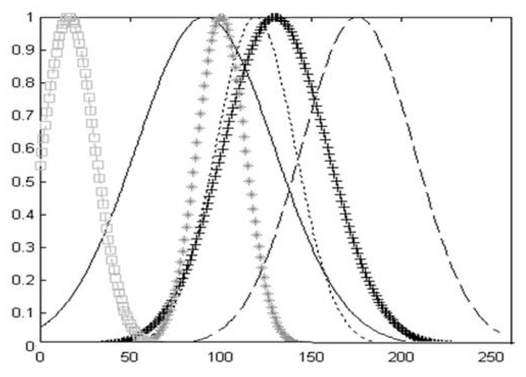
The normalized approximate Gaussian distributions of blood, tissue and instruments from Table 1. From left to right: blood (□□□), cardiac tissue (——), acetal (***), fiber glass (---), epoxy (+++) and wood (– – –). The distribution of wood is best separated from that of tissue, while the distribution of acetal is superimposed over that of tissue.

In-Vitro Experiments

The algorithm was first tested using 3D in-vitro data from a water tank trial. The training sets and test data were acquired under similar imaging conditions using the same type of instrument. All data was acquired with a Sonos 7500 Live 3D Echo scanner (Philips Medical Systems, Andover, MA, USA). An acetal rod was placed in the tank in the proximity of a flat bovine muscle tissue sample approximately 2 cm thick. There was no contact between the instrument and the tissue. Figure 6 shows detection results at various algorithm stages in 2D slices. In Figure 7 we present the 3D volumes showing in-vitro instrument detection.

Figure 6.

Tank data: (a) a 2D slice of a 3D US image of an acetal rod approaching a tissue sample in a water tank; (b) detection results after EM, where the instrument is shown in white, the tissue in gray, and the blood in black; (c) detection results employing neighboring information; (d) detection results after PCA.

Figure 7.

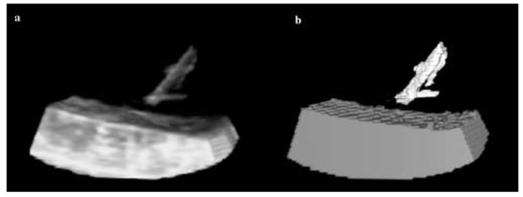
3D in-vitro data: (a) the US image of an acetal rod approaching a tissue sample in a water tank; (b) detection results where the instrument is shown in white, the tissue in gray, and the blood in black.

In-Vivo Experiments

The second segmentation example detects a wooden instrument during an intracardiac operation on a porcine beating heart. This in-vivo US image shows the wooden rod in contact with the cardiac tissue. Figure 8 shows the detection stages in in-vivo images. After PCA, the instrument is generally well detected, but FPs occur at the contact with tissue. WT eliminates the residuals and segments the instrument correctly. Figure 9 presents the 3D US segmentation results.

Figure 8.

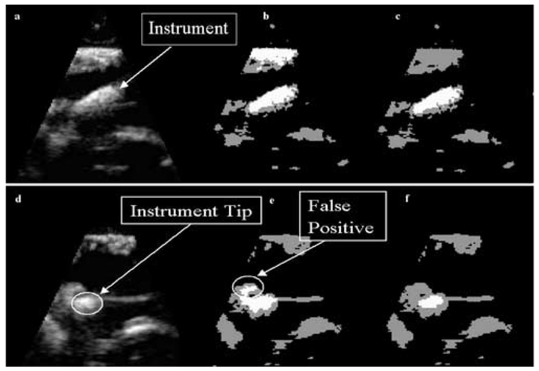
In-vivo data: (a) a 2D slice of a 3D US image of a porcine heart with a wooden rod inside acquired during an intracardiac beating-heart procedure; (b) detection results after the analysis of intensity distributions, where the instrument appears white, tissue gray and blood black; (c) the segmentation of instrument and tissue after PCA: the instrument appears correctly segmented, but this is not the case for the whole 3D US image; (d) a slice of the 3D US image at a different location, where the tip of the instrument touches the tissue; (e) detection results after PCA at the new location showing FP; (f) improved results employing the watershed algorithm.

Figure 9.

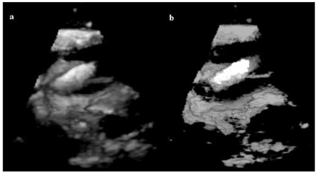
3D in-vivo results: (a) a 3D US image of a porcine heart with a wooden rod inside (in contact with the tissue); (b) 3D segmentation results for image (a) with the instrument shown in white, blood in black and tissue in gray (the gray scale appearance is an effect of the rendering algorithm).

For illustration, we compared the segmentation results of the EM framework to that of basic thresholding into three classes: dark, mid-gray and bright. We took into consideration the computed distributions of blood, tissue and instrument and present the results that reflect best the segmentation of instrument. Some comparative results are shown in Figure 10. While our EM scheme outperforms thresholding, the figure also reflects that EM plays a limited role in the segmentation algorithm.

Figure 10.

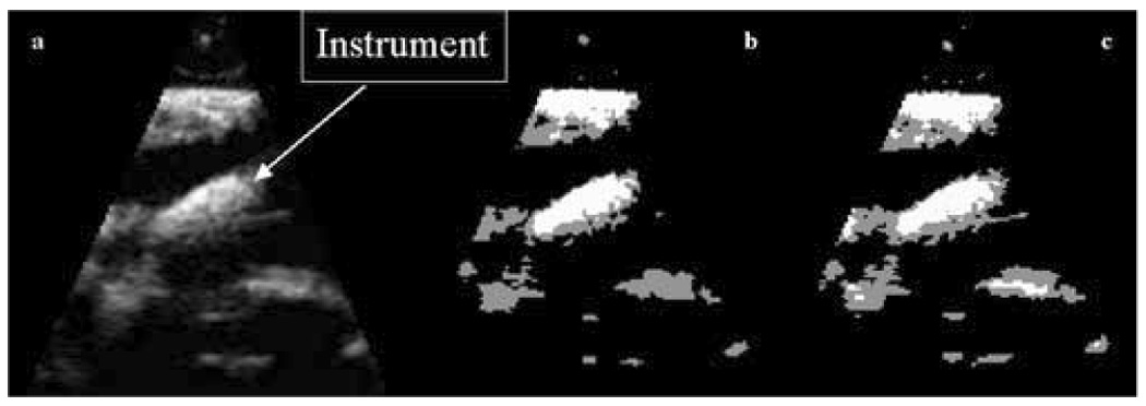
Comparative segmentation results: (a) a 3D US image of a porcine heart with a wooden rod inside; (b) results of EM segmentation; (c) results of thresholding segmentation.

More results from in-vivo intra-cardiac interventions are presented in Figure 11. We segment two instruments made of threaded stainless steel: one coated with fiber glass and the second coated with epoxy. The fiber glass rod has a clean appearance with very small reverberations and tip artifact. Although the epoxy instrument has better separated distribution from that of tissue, the presence of reverberations and the contact with tissue on the length of the rod, make this case more challenging. Comparison with expert-annotated images shows the correct segmentation and position of the instrument shaft in all situations. The instrument orientation is extracted from its principal components.

Figure 11.

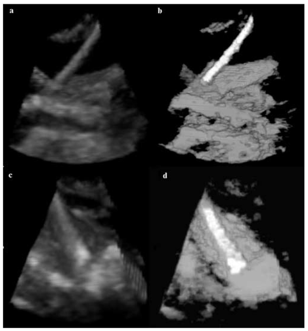
3D in-vivo results: (a) a 3D US image of a porcine heart with threaded stainless steel rod coated with fiber glass; (b) 3D segmentation results for image (a); (c) a 3D US image of a porcine heart with threaded stainless steel rod coated with epoxy; (d) 3D segmentation results for image (c).

In all our in-vitro data, the tip was correctly segmented with no error. The golden standard was provided by expertly segmented instrument tips, which were selected as the voxels (one voxel for each instrument) at the inner end of the instrument facing the US probe (the correctly visible surface of the instrument is oriented towards the probe in US images). The algorithm segmented tip is the end voxel of the segmented instrument facing the US probe and the segmentation error is the Euclidean distance between the expert and algorithm segmented tips. The combination of intensity and shape analysis finds the tip of the instrument in in-vivo images without contact between the instrument and tissue with very small errors. The segmentation is more difficult when the instrument rod touches the heart tissue. We used 50 in-vivo 3D US images with instruments placed in porcine hearts: 25 threaded steel rods coated with epoxy and 25 threaded steel instruments coated with fiber glass. Overall, the tip segmentation error in in-vivo data was of 1.77+/−1.40 voxels.

DISCUSSION

We presented a multi-step algorithm for the detection of instruments in 3D US images. It begins with finding an estimate of the statistical distributions of the classes of objects we aim to segment. Our database consists of images acquired at different times and locations, but on the same type of US machine and probe. The method is not sensitive to image acquisition conditions. It suffices to determine the distribution functions of blood and tissue once for all the subsequent segmentations, presuming that the clinician adjusts the scan parameters to derive a good image of the tissue, as it is customary in clinical practice. However, the instrument probability distribution function (pdf) is unique to the type of material it is made from. Hence, for each type of instrument material, there will be a different pdf and the method requires a small database of material types and statistics. The instrument material may be standardized for a particular procedure, or the user interface may allow the selection of the instrument material used.

Next, the image voxels are assigned to three classes: blood, tissue and instrument. The statistical classification converges to three stable classes of voxels, but the uncertainty at the overlap of the Gaussian distributions of instrument and tissue brings labeling errors. Hence, some spatial information is required. A neighboring information step improved the segmentation results of in vitro data, but was not essential in the in vivo experiments. This is due to the simpler image information in the tank trials (no contact between instrument and tissue and simpler shapes) and the superimposed distributions of acetal and cardiac tissue. For complex in-vivo data, this type of simple spatial information improves the segmentation of the instrument, but introduces errors in tissue.

US enables guided interventions, but instruments have not been designed for US. We used wood in our initial experiments, as some surgeons use wood for manipulation for the good visibility in US imaging, but not in surgery. Wood also has the best pdf separation from tissue, which helped designing our algorithm. For the rest of our experimental in-vivo results, we used coated threaded steel. These newly developed instruments have an enhanced surface visibility in ultrasound images, due to the reduction in specularity. The echo amplitude mean and standard deviation of the instrument is also better separated from that of the tissue, for these classes of instruments.

PCA is employed as a statistical measure of shape. The analysis is based on the assumption that instruments are shaped like rods, long and thin. We analyze the connected components in the image and keep only the candidates that satisfy the shape requirements. The major source of remaining errors is the contact area between instrument and tissue. Finally, WT separates the instrument from tissue in critical areas in a fine to coarse approach. This WT-PCA hybrid approach uses first PCA to reduce the computational expense and speed up the algorithm. WT then reduces the segmented volume of instrument to the portion of the instrument shaft oriented towards the US probe. This produces smaller errors in the approximation of the instrument axis. To this extent, we assume that there is only one instrument in every image.

Calibrated systems would aim for instrument mean and standard deviation to be constant, given a certain depth. The visual adjustment of TGC settings helps and we kept this in mind during image acquisition, although the system was not truly calibrated. This was possible in our cardiac applications, where the depth range of the instrument does not vary much when the US probe is placed on the atrial wall. We computed the statistics only once for tissue, blood and each type of instrument and included voxels from the entire instrument shaft over the depth-range. Although there would be some difference in the appearance of an instrument from one acquisition to the next, the relation between the three distributions (blood, tissue and instrument) does not change, as demonstrated by our segmentation results. This relation was enhanced by the use of instruments designed to separate the echo amplitude mean and standard deviation of the instrument from that of the tissue (Huang et al. 2006).

The implementation of the algorithm is done in Matlab version 7 (The MathWorks, Inc.) on a Pentium 4 machine with 1GB RAM and 2.40 GHz processor. Running the algorithm on a 128×48×208 3D US volume takes approximately 70s. Our segmentation results are for single 3D images, but a potential major application is tracking instrument movement in 4D US clinical images. Clinical applications will clearly require considerable speed improvements; the present implementation was not optimized, and considerable acceleration may be achieved, especially in the iterative portions of the algorithm, by initializing each new image with the result of the previous image.

For surgical guidance purposes, it would be useful to fit the instrument shape into the 3D US volume at the location of the surgical instrument. This is beyond the scope of this paper, which focuses the first step of this process, segmentation of instruments in US data. In 3D US, instruments appear as irregular clouds of voxels, where reverberations and tip artifacts are visible, but do not exist. For this reason, our algorithm detects the region of the instrument shaft oriented toward the US probe, which is the brightest part of the instrument in the 3D US volume. Following segmentation, a priori information on the size of the instrument (length and diameter), combined with the closest image boundary to the instrument and an estimation of the instrument tip, can be used to superimpose in the image a model mimicking the ideal appearance of the instrument. An example is presented in Figure 12, where a 2D slice of a 3D volume with a fiber glass coated rod is segmented. Note that part of the area of the instrument as appearing in US is left labeled as tissue (in gray). The area labeled as instrument gives the best estimate of the real instrument axis and position, as approximated by the white rectangle.

Figure 12.

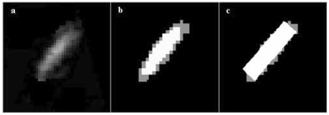
Instrument orientation and position: (a) a 2D slice of a 3D volume with part of a threaded steel rod coated with fiber glass; (b) the segmented instrument shaft (white=instrument, gray=tissue); (c) the superimposed true shape of the instrument over the segmented result, as it appears in the 2D slice; the rectangle wraps the segmented result along its main principal axis.

This work considered a simple statistical model of the tissue, blood, and instrument classes. While it achieves good segmentation, more sophisticated treatment may improve performance. Image normalization is known to reduce the deviation of the point-spread functions of object classes. We will investigate the impact of normalization to make the statistical classification more robust. Neighborhood analysis and connectivity through Markov Random Fields should also help to correct segmentation errors. More spatial and statistical information using the instrument shape and principal factor analysis (Gonzalez Ballester et al. 2005) will be implemented for a larger variety of instrument materials. Our segmentation results can be used as an initialization step for tracking instruments in 4D echocardiography. The computational speed will be a priority for real-time interventional applications.

REFERENCES

- Angelini ED, Homma S, Pearson G, Holmes JW, Laine AF. Segmentation of real-time three-dimensional ultrasound for quantification of ventricular function: a clinical study on right and left ventricles. Ultrasound Med Biol. 2005;1(9):31143–31158. doi: 10.1016/j.ultrasmedbio.2005.03.016. [DOI] [PubMed] [Google Scholar]
- Cannon JW, Stoll JA, Salgo IS, Knowles HB, Howe RD, Dupont PE, Marx GR, del Nido PJ. Real Time 3-Dimensional Ultrasound for Guiding Surgical Tasks. Computer Aided Surgery. 2003;8:82–90. doi: 10.3109/10929080309146042. [DOI] [PubMed] [Google Scholar]
- Couvreur C. The EM Algorithm: A Guided Tour. IEEE European Workshop on Computationally Intensive Methods in Control and Signal Processing. 1996:115–120. [Google Scholar]
- Ding M, Fenster A. Projection-based Needle Segmentation in 3D Ultrasound Images. Computer Aided Surgery. 2004;9(5):193–201. doi: 10.3109/10929080500079321. [DOI] [PubMed] [Google Scholar]
- Downing SW, Herzog WR, Jr, McElroy MC, Gilbert TB. Feasibility of Off-pump ASD Closure using Real-time 3-D Echocardiography. Heart Surgery Forum. 2002;5(2):96–99. [PubMed] [Google Scholar]
- Gonzalez Ballester MA, Linguraru MG, Reyes Aguirre M, Ayache N. Fitzpatrick JM, Reinhardt JM, editors. On the Adequacy of Principal Factor Analysis for the Study of Shape Variability. SPIE Medical Imaging. 2005;5747:1392–1399. [Google Scholar]
- Grau V, Mewes AUJ, Alcaniz M, Kikinis R, Warfield SK. Improved Watershed Transform for Medical Image Segmentation Using Prior Information. IEEE Trans Medical Imaging. 2004;23(4):447–458. doi: 10.1109/TMI.2004.824224. [DOI] [PubMed] [Google Scholar]
- Hopkins RE, Bradley M. In-vitro Visualization of Biopsy Needles with Ultrasound: A Comparative Study of Standard and Echogenic Needles Using an Ultrasound Phantom. Clin Radiology. 2001;56(6):499–502. doi: 10.1053/crad.2000.0707. [DOI] [PubMed] [Google Scholar]
- Huang J, Dupont PE, Undurti A, Triedman JK, Cleveland RO. Producing Diffuse Ultrasound Reflections from Medical Instruments Using a Quadratic Residue Diffuser. Ultrasound in Medicine and Biology. 2006;32(5):721–727. doi: 10.1016/j.ultrasmedbio.2006.03.001. [DOI] [PubMed] [Google Scholar]
- Jackson JE. A User's Guide to Principal Components. New York: John Wiley & Sons, Inc.; 1991. [Google Scholar]
- Lin N, Yu W, Duncan JS. Combinative Multi-Scale Level Set Framework for Echocardiographic Image Segmentation. Medical Image Analysis. 2003;7(4):529–537. doi: 10.1016/s1361-8415(03)00035-5. [DOI] [PubMed] [Google Scholar]
- Mitchell SC, Bosch JG, Lelieveldt BPF, van der Geest RJ, Reiber JHC, Sonka M. 3-D active appearance models: segmentation of cardiac MR and ultrasound images. IEEE Trans Medical Imaging. 2002;21(9):1167–1178. doi: 10.1109/TMI.2002.804425. [DOI] [PubMed] [Google Scholar]
- Nichols K, Wright LB, Spencer T, Culp WC. Changes in Ultrasonographic Echogenicity and Visibility of Needles with Changes in Angles of Insonation. J Vasc Interv Radiol. 2003;14(12):1553–1557. doi: 10.1097/01.rvi.0000099527.29957.a6. [DOI] [PubMed] [Google Scholar]
- Novotny PM, Cannon JW, Howe RD. Tool Localization in 3D Ultrasound. Medical Image Computing and Computer Assisted Intervention (MICCAI) 2003;2879:969–970. LNCS. [Google Scholar]
- Ortmaier T, Vitrani MA, Morel G, Pinault S. Robust Real-Time Instrument Tracking in Ultrasound Images for Visual Servoing. In: Fitzpatrick JM, Reinhardt JM, editors. SPIE Medical Imaging. Vol. 5750. 2005. pp. 170–177. [Google Scholar]
- Paragios N. A Level Set Approach for Shape-driven Segmentation and Tracking of the Left Ventricle. IEEE Trans Med Imaging. 2003;22(6):773–786. doi: 10.1109/TMI.2003.814785. [DOI] [PubMed] [Google Scholar]
- Roerdinck JBTM, Meijster A. The Watershed Transform: Definitions, Algorithms and Parallelization Strategies. Fundamenta Informaticae. 2000;41:187–228. [Google Scholar]
- Shapiro LM, Kenny A. Cardiac Ultrasound. Manson Publishing. 1998 [Google Scholar]
- Stoll JA, Novotny PM, Howe RD, Dupont PE. Real-time 3D Ultrasound-based Servoing of a Surgical Instrument; Proceeding of IEEE International Conference on Robotics and Automation; 2006. pp. 613–618. [Google Scholar]
- Suematsu Y, Martinez JF, Wolf BK, Marx GR, Stoll JA, DuPont PE, Howe RD, Triedman JK, del Nido PJ. Three-dimensional Echo-guided Beating Heart Surgery without Cardiopulmonary Bypass: Atrial Septal Defect Closure in a Swine Model. Journal Thoracic Cardiovascular Surgery. 2005;130(5):1348–1357. doi: 10.1016/j.jtcvs.2005.06.043. [DOI] [PubMed] [Google Scholar]
- Vincent L, Soille P. Watersheds in Digital Spaces: An Efficient Algorithm Based on Immersion Simulations. IEEE Tran. Pattern Analysis and Machine Intelligence. 1991;13(6):583–598. [Google Scholar]
- Xiao G, Brady JM, Noble JA. Segmentation of Ultrasound B-Mode Images with Intensity Inhomogeneity Correction. IEEE Trans Medical Imaging. 2002;21(1):48–57. doi: 10.1109/42.981233. [DOI] [PubMed] [Google Scholar]