Prediction of protein loop structures using a local move Monte Carlo approach and a grid-based force field

Abstract

We have developed an improved local move Monte Carlo (LMMC) loop sampling approach for loop predictions. The method generates loop conformations based on simple moves of the torsion angles of side chains and local moves of backbone of loops. To reduce the computational costs for energy evaluations, we developed a grid-based force field to represent the protein environment and solvation effect. Simulated annealing has been used to enhance the efficiency of the LMMC loop sampling and identify low-energy loop conformations. The prediction quality is evaluated on a set of protein loops with known crystal structure that has been previously used by others to test different loop prediction methods. The results show that this approach can reproduce the experimental results with the root mean square deviation within 1.8 Å for all the test cases. The LMMC loop prediction approach developed here could be useful for improvement in the quality the loop regions in homology models, flexible protein–ligand and protein–protein docking studies.

Introduction

Secondary structures of proteins can be classified into helices, strands and loops. Loops are irregular regions connecting two regular secondary structure segments (helices or sheets) in proteins. Loops are usually variable in both sequence and structure even in the same protein family, which makes loops the most difficult regions to model by comparative modeling approaches. The accuracy of homology models is generally lowest in loop regions. However, loops are important for protein functions, and play critical roles in protein recognition (Bajorath and Sheriff, 1996; Fetrow et al., 1998), ligand binding (Joseph et al., 1990; Ragona et al., 2003), and enzyme activities (Wlodawer et al., 1989; Liu et al., 2004). Consequently, loop modeling has become one of the important challenges in protein structure prediction, and has been described as a mini protein-folding problem (Fiser et al., 2000).

Over the last two decades, many different loop-modeling approaches have been developed. In general, loop-modeling methods can be divided into two classes: database search (Greer, 1980; Jones and Thirup, 1986; Chothia and Lesk, 1987; Fernandez-Fuentes et al., 2006; Peng and Yang, 2007) and ab initio (Fine et al., 1986; Moult and James, 1986; Bruccoleri and Karplus, 1987; Rohl et al., 2004; Mehler et al., 2006; Zhu et al., 2006; Soto et al., 2008; Spassov et al., 2008) methods. In the database search method, a protein structure database is searched to find main chain segments that fit the anchor regions of a loop. In the ab initio methods, a large number of conformations are generated from special algorithms, and followed by their energy evaluations based on some particular scoring or energy functions. These methods have been comprehensively reviewed elsewhere (van Vlijmen and Karplus, 1997; Fiser et al., 2000; Soto et al., 2008).

Recently, ab initio approaches for loop modeling showed more accurate predictions than database search approaches, especially for long loops (Xiang et al., 2002; Michalsky et al., 2003; Jacobson et al., 2004; Zhu et al., 2006; Soto et al., 2008). The accuracy of ab initio approaches depends on two factors: (i) the quality of loop conformational sampling algorithms; (ii) the accuracy of the scoring or energy functions used for ranking the sampled loop conformations. A number of loop conformational sampling algorithms have been developed, including analytical methods (Go and Scheraga, 1970; Bruccoleri and Karplus, 1985), random tweak (Fine et al., 1986; Shenkin et al., 1987; Smith and Honig, 1994), systematic conformational search (Moult and James, 1986; Bruccoleri and Karplus, 1987; Brower et al., 1993), genetic algorithms (McGarrah and Judson, 1993; Ring and Cohen, 1994), bond scaling (Zheng et al., 1993; Rosenbach and Rosenfeld, 1995; Zheng and Kyle, 1996), and Monte Carlo (MC) (Higo et al., 1992; Carlacci and Englander, 1993; Collura et al., 1993; Zhang et al., 1997). Scoring or energy functions that have been used include molecular mechanics force field (Cornell et al., 1995; MacKerell et al., 1998) and statistical potentials (Sippl, 1990; Samudrala and Moult, 1998; de Bakker et al., 2003), combined with different implicit solvent models, such as distance-dependent dielectric model (Bruccoleri and Karplus, 1987; Das and Meirovitch, 2001), finite difference Poisson–Boltzmann model (Smith and Honig, 1994), and Generalized Born (GB) solvation model (Rapp and Friesner, 1999).

In the present study, we employ an improved LMMC sampling approach, combined with grid mapping potentials for loop predictions. Local move (also referred to as ‘window move’) starts with changing one torsion angle (called the driver torsion) followed by the adjustment of the six subsequent torsions to allow the rest of the chain to remain in its original position while preserving all bond lengths and bond angles. The pioneering work on local move was done by Go and Scheraga (1970), who developed a solution for the system of equations defining the values of the six torsion angles that preserve the backbone bond lengths and angles. Hoffmann and Knapp first applied the local move method in a MC simulation of polyalanine folding that included a suitable Jacobian (Dodd et al., 1993), required for maintaining detailed balance. They demonstrated that this method samples the conformational space more efficiently than single move (Hoffmann and Knapp, 1996). The method has been further tested on proline-containing peptides (Wu and Deem, 1999a), proteins and nucleic acids (Dinner, 2000). Mezei introduced the ‘reverse proximity criterion’ for filtering all possible loop closure solutions to select the most structurally conservative one, and tested it on a solvated lipid bilayer (Mezei, 2003). Here we present an improved efficiency LMMC sampling for loop prediction, by substituting the rest of the protein with a grid-based force field, which includes van der Waals, electrostatics, hydrophobic, hydrogen bond potentials and solvation effects. Our loop prediction approach was then evaluated by comparing its predictions with those that have been published (van Vlijmen and Karplus, 1997; Deane and Blundell, 2000; Fiser et al., 2000; Deane and Blundell, 2001). The results show an improvement in accuracy for loop prediction, which can be attributed to the powerful LMMC sampling technique and the accurate grid-based energy function.

Methods

LMMC sampling

The proper execution of a local torsion move that changes the shortest backbone segment requires the solution of several problems. First, having changed a torsion angle by a randomly selected amount, the determination of the additional six torsion angle values poses a problem in geometry – several algorithms have been presented for its solution. This problem may have up to 16 solutions (Wedemeyer and Scheraga, 1999). The strategies suggested for choosing among the solutions include random selection (Dodd et al., 1993), selection weighted by the Jacobian and a Rosenbluth-type weight, supplemented by generating side chain conformations with the configurational bias method (Deem and Bader, 1996; Wu and Deem, 1999b) corresponding to each solution (Hoffmann and Knapp, 1996) or the one that results in the smallest change (Mezei, 2003). Each strategy has its corresponding acceptance filter to maintain microscopic reversibility, leading to Boltzmann-distributed conformational ensembles.

Here we used the reverse proximity acceptance criterion for LMMC method. In contrast to previous methods, not all possible loop closures are considered, but only the most structurally conservative one, selected by filtering local moves with the ‘reverse proximity criterion’. The method is ergodic, and was shown to be significantly more efficient than previous methods when applied to a fully solvated hydrocarbon chain with bulky side chains as well as a fully solvated lipid bilayer (Mezei, 2003).

Potential energy maps

To increase the computing speed of energy evaluations for LMMC loop sampling, we developed a grid-based force field, which includes van der Waals, electrostatics, hydrophobic, and hydrogen bond potentials to replace the protein structure and solvent effect. For the explicitly represented loop region, we used the all-atom CHARMM force field (Brooks et al., 1983) with sigmoidal distance-dependent dielectric constants (Mehler and Solmajer, 1991), hydrogen bond and hydrophobic terms (Huey et al., 2007). To increase the accuracy of energy evaluations, we used a cubic grid box size of 161 × 161 × 161 with a fine grid resolution of 0.25 Å.

Electrostatics.

Coulomb potential ϕ(r), with a sigmoidal distance-dependent dielectric function was used to model solvent screening, based on the work of Mehler and Solmajer (1991):

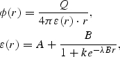where Q is partial charge; B= e0− A; e0 = 78.4 (the dielectric constant of bulk water at 25°C); A= 6.02944, λ = 0.018733345 and k = 213.5782 are parameters (See Supplementary data available at PEDS online). The original parameter set has been modified to produce better results comparing with the GB model. When the distance between two charges is <1.32 Å, a dielectric constant of 8 is used.

van der Waals.

A 12-6 Lennard-Jones potential was used:

where the C₁₂ and C₆ Lennard-Jones parameters of five atom types (united atoms C, N, O, S and polar H) are from the AUTODOCK program (Morris et al., 1998).

Desolvation.

The general approach of Wesson and Eisenberg (1992) was used, and the atomic solvation parameters were calculated based on the absolute partial charge on the atom:

where i= index of atoms in the ligand; j = index of atoms in the receptor; W_desolv= linear regression coefficient or weight for the desolvation free energy term; S_i = solvation term for atom i; V_i = atomic fragmental volume of atom i; r_ij = distance between atom i and atom j (in Å); σ = Gaussian distance constant = 3.5 Å. The parameters are obtained from the AUTODOCK4 program (Huey et al., 2007). Only non-polar carbon atoms (the absolute value of charge is <0.2) were used for desolvation energy calculations.

Hydrogen bond.

A 12-10 potential was used:

where C₁₂ and C₁₀ are 12-10 parameters. We developed the hydrogen bond parameters based on different donor and acceptor types (See Supplementary data available at PEDS online). The hydrogen bond energies are angle-dependent (the angle (θ) of acceptor atom-polar hydrogen-donor atom), and were calculated only when the distance between hydrogen and acceptor atoms was between 1.65 and 3.00 Å, and 90° <θ≤180°.

System setup

The coordinates of the protein are partitioned into two sets: the loop, with a few anchoring atoms (that will be kept fixed) and the bulk of the fixed atoms. The list of loop atoms is used to generate the list of torsions, both side chain and backbone. The maximum possible extent the loop conformations can sample also has to be established to define the limits of the grid box. In a preparatory calculation the electrostatic, van der Waals, desolvation and hydrogen bond acceptor energies are calculated at every grid point. However, hydrogen bonds where the loop hydrogen is the donor depend on the bond orientation between the donor hydrogen and its heavy atom, and thus they have to be calculated explicitly. This necessitated the generation of a list of hydrogen bond acceptors on the fixed part of the protein, and a link list, based on a ∼3 Å grid, listing the possible hydrogen bond acceptors for loop atoms falling into each of these grids. For the calculations designed to reproduce the crystal structure of the loop the mobile loop atoms were removed and regenerated by the Modloop server (http://modbase.compbio.ucsf.edu/modloop///modloop.html) (Fiser and Sali, 2003) to provide an initial configuration independent of the crystal structure.

MC loop sampling and simulated annealing

To improve the efficiency of LMMC loop sampling, we used a simulated annealing approach to identify the local minima on the energy surface. First, we sampled loop conformations at the high temperature of 5000 K to explore the loop conformational space. In order to lower the energy barriers and thereby speeding up the sampling of the conformational space we used reduced map potentials in this phase of the calculations: every grid point potential >2 kcal/mol was set to 2 kcal/mol. The loop conformations with the lowest total energies were recorded over every 50 000 MC steps. The saved conformations were clustered with the SIMULAID program (http://inka.mssm.edu/~mezei/simulaid) using the loop backbone root mean square deviation (RMSD) as the distance measure. The clustering algorithm used picks the element that has the largest number of conformations within the distance cutoff and makes it a cluster. This cluster is then removed and the procedure is repeated on the remaining configurations until no more configurations are left. The lowest energy loop conformation in each cluster was selected as the representative loop structure. Each cluster-representative loop structure was used as the initial structure to conduct simulated annealing simulations from 5000 to 20.68 K by using the Exponential Cooling Scheme (also called geometric cooling scheme) with scaling factor 0.95, for 5.35 million MC steps; followed by Linear Cooling Scheme from 20.68 to 0.68 K for 200 000 MC steps, and each segment took 50 000 MC steps. Unlike during the initial loop sampling stage, we used a non-reduced potential map to accurately calculate the interaction energies between the loop and the rest of the protein. In general, the more clusters we use, the better prediction results we expect to get. However, computational costs will be increased in proportion to the number of clusters. We also found that a slower cooling process can improve the accuracy of loop predictions; similarly, it will increase the computational costs as well.

Results and discussion

To evaluate the performance of our newly developed grid-based LMMC loop prediction approach, we applied it to a test set of protein loops, which was originally used by van Vlijmen and Karplus (1997), and later by Fiser et al. (2000), and by Deane and Blundell (2000; 2001), Michalsky et al. (2003), and Rohl et al. (2004).

Loop test set

The loop test set contains 14 protein loop crystal structures, with the loop lengths ranging from four to nine residues. We subjected all the protein structures in the test set to 1000 steps of Steepest Descent (SD) energy minimization by using CHARMM program with GB solvation module (Im et al., 2003). Then the loops were removed from the protein structures. Since we have not developed a loop generation program, we regenerated each loop by the Modloop web server (Modloop generates only one loop for each structure) (Fiser and Sali, 2003) to obtain an initial conformation for our high-temperature run. Note, however, that any available program can be used to generate the initial loop structures with reasonable bond lengths and bond angles. Since we will sample the entire loop conformational space by LMMC method at very high temperature, the initial loop conformations are not be expected to affect the final loop prediction results. Each newly generated loop region in proteins was refined by the same method and protocol for energy minimization described earlier.

Crystal packing

Protein structures in the test set were determined by x-ray crystallography. Thus it is possible that loop conformations could be affected by crystal packing. We have reconstructed the crystal packing protein structures for all the proteins in the test set by using Swiss PDB Viewer program (http://www.expasy.org/spdbv/) (Guex and Peitsch, 1997). We found that in six out of the 14 crystal structures, loops are located at the interface between subunits in the crystal, and thus native loop conformations could be affected by the crystal packing. So the related monomers in these structures need to be included in loop predictions if the goal is to model the loop conformation in these crystals. However, the effect of crystal packing in this loop test set has not been considered in previous studies. We expect that this will improve the prediction due to the additional restraints imposed on the loops. In this work we included the crystal packing information by introducing additional related monomer structures for loop predictions. A typical crystal packing example is shown in Fig. 1, in which the protein (3grs) forms a trimer in the crystal packing, the loops to be predicted are very close, and located at the interface of the two monomers. This crystal packing is thus critical to the formation of this conformation observed in the experiment, and it must be included for the evaluation of loop predictions.

Fig. 1.

Protein (3grs) forms trimer in the crystal packing. The loops to be predicted are located at the interface of two monomers. The gray wires represent the protein structures in trimer form; black sticks represent loops [L1, L2 and L3 (83–89) are from different monomers] to be predicted.

Loop sampling and clustering

Two additional N- and C-terminal residues are included as fixed anchors of each loop structure for MC local move sampling. During the LMMC sampling, the loop side chain torsion angles and backbone torsion angles phi (ϕ) and psi (ψ) are allowed to change by any amount, while the backbone torsion angles omega (ω) are allowed to change <90° from their original values (∼180°). Two types of MC moves are performed: simple moves (single torsion angle rotations) and local moves.

We sampled each loop in the test set at 5000 K for 100 million MC steps, and recorded the lowest total energy loop conformations over every 50 000 MC steps. We found the use of the reduced maps at this stage of the calculation was essential to enable crossing the high-energy barriers between separate local minima during loop conformation sampling.

The loop conformations extracted were first clustered to yield 100 clusters. If the backbone RMSD cutoff resulting in 100 clusters exceeded 1 Å then the clustering was repeated for better results with 1 Å cutoff, resulting in more clusters. We selected one representative loop structure with the lowest total energy from each cluster as the initial loop structure for the following simulated annealing simulations. A typical example of loop sampling is shown in Figs 2 and 3. From Figs 2 and 3 we can see that although the initial loop structure is 6.0 Å (RMSD based on the backbone atoms of loops) away from the crystal loop structure [5cpa (231–237)], LMMC sampling can cover large conformational space that includes the vicinity of the crystal loop conformation (as demonstrated in Fig. 2). The largest RMSD between any two sampled loop conformations is 8.77 Å.

Fig. 2.

Loop structures of 5cpa (231–237) produced by LMMC method at 5000 K and followed by clustering to generate 100 representative conformations. Black stick represents the crystal loop structure, and gray wires represent the 100 representative loop conformations.

Fig. 3.

Total energies versus RMSD of the 100 representative loop conformations of 5cpa (231–237) from LMMC sampling (before simulated annealing). The RMSD calculations are based on the backbone atoms of the crystal and representative loop structures.

MC simulated annealing

The loop structure with the lowest total energy generated by each MC simulated annealing simulation was saved as a putative prediction of loop structure. For each system the loop conformation with the lowest total energy was selected as the final predicted loop structure. Beside the RMSD between the final prediction and the crystal structure, the quality of a scoring function is usually characterized with the plot of the total energy versus RMSD. A typical example [8tln (248–255)] is shown in Fig. 4 (RMSD was based on backbone atoms). The RMSD difference of predicted loop configurations of 8tln (248–255) before and after LMMC simulated annealing is shown in Supplementary Figure 5 available at PEDS online, and the average RMSD before and after MC simulated annealing for all cases is listed in Supplementary Table I available at PEDS online. From Fig. 4 we can see that the loop conformation with the lowest total energy also corresponds to the lowest RMSD from the crystal loop structure. We also calculated the correlation efficients between the interaction energies and the RMSD, and listed in Supplementary Table I available at PEDS online, which shows that there are no correlations. The crystal, initial and predicted loop structures in the protein of 8tln (248–255) are shown in Fig. 5. As can be seen from the figure, this loop is located at the interface of two monomers and is thus interacting with both monomers; therefore the crystal packing information was included for our MC loop prediction. The RMSD of the final predicted loop is 0.67 Å from the crystal loop structure.

Fig. 4.

Total energies versus RMSD [100 predicted loop conformations (the energies >27 900 kcal/mol are not shown) of 8tln (248–255) from LMMC simulated annealing]. The RMSD calculations are based on the backbone atoms of the crystal and predicted loop structures.

Fig. 5.

Crystal, initial and predicted loop structures in the protein dimer of 8tln (248–255). The gray wires represent the crystal structures, the gray stick represents the initial loop structure (6.0 Å of RMSD from crystal loop structure), and the black stick represents the MC predicted loop structure (0.67 Å of RMSD from crystal loop structure).

Energy minimization

We also tested whether further energy minimization will improve the accuracy of predicted loop structures. We performed energy optimization on the lowest energy structures for 1000 steps SD (loop only) by using GB implicit solvent model in CHARMM program, and found that nine out 14 structures have been slightly improved comparing with crystal structures while the remaining five became slightly worse (Table I).

Table I.

Comparison of loop prediction results from LMMC simulated annealing method and others [the results are based on the backbone global RMSD (in Å) between the crystal and predicted loop structures]

PDB code	Loop	Length	LMMC	LMMC-MM	van Vlijmen and Karplus	CODA	PETRA	Fiser	LIP	Rosetta
2apr	76–83	8	0.37	0.29	5.16	2.2	2.6	1.31	0.50	2.54
8abp	203–208	6	0.29	0.22	0.28	0.8	2.5	0.38	0.79	0.56
2acta	198–205	8	1.52	1.69	1.58	3.1	1.5	1.04	0.13	3.79
8tlna	E32–E38	7	0.46	0.25	3.70	1.9	—	2.03	0.24	2.62
3grsa	83–89	7	1.15	1.20	4.55	1.4	2.0	0.42	2.13	0.97
5cpa	231–237	7	1.05	0.95	2.14	0.2	1.3	0.95	0.23	1.22
2fb4a	H26–H32	7	1.10	1.09	1.62	0.4	1.9	4.20	0.19	1.79
2fbja	H100–H106	7	0.85	0.86	0.49	1.4	3.2	0.84	9.00	0.98
8tlna	E248–E255	8	0.63	0.50	1.83	1.8	—	0.87	0.61	1.52
3sgb	E199–E211	9	1.68	1.73	1.79	—	—	0.28	0.22	1.10
3dfr	20–23	4	0.46	0.37	2.64	0.4	1.7	1.15	1.07	0.80
3dfr	89–93	5	0.72	0.75	1.62	0.6	1.2	1.02	3.13	0.96
3dfr	120–124	5	0.57	0.46	0.47	0.7	1.2	0.26	1.92	0.76
3blm	131–135	5	0.25	0.11	0.82	0.2	1.8	0.16	0.24	0.43

^aCrystal packing information is included for loop prediction by LMMC method only.

Comparison of loop prediction results

We predicted the loop structures for the entire test set by using LMMC simulated annealing method with the same protocol as described earlier. The predicted loop results together with the results from others are listed in Table I. It should be stressed that, unlike in our calculations, crystal packing was not considered by in the other prediction methods, which could have some potential effect on these prediction results (more likely positive effect due to the additional constraints for loops). Six out of 14 native loop conformations in this test set could be affected by crystal packing. From Table I we can see that 12 out of 14 of the loop predictions in our study are better than those from van Vlijmen and Karplus method; 10 out of 13 are better than those from the CODA method; 10 out of 11 are better than those from PETRA method; eight out of 14 are better than those of Fiser; nine out of 14 are better than those from LIP method; 11 out of 14 are better than those from Rosetta method. The worst RMSD of loop predictions from our method is 1.73 Å comparing with 5.16 Å from van Vlijmen and Karplus method; 3.1 Å from CODA method; 3.2 Å from PETRA method; 4.2 Å from Fiser method; 9.0 Å from LIP method; 3.79 Å from Rosetta method. Note also that—unlike in the other methods—all our predictions had global RMSD < 2 Å, the threshold that is considered to define a good loop prediction (Fiser et al., 2000). However, our method is significantly slower than the others in this comparison, representing the ‘price’ of the increased accuracy of our loop predictions.

Computational costs

The first stage of LMMC sampling for 100 million MC steps takes <20 h/CPU (Apple G5 processor). Each LMMC simulated annealing simulation for 6 million MC steps takes <1 h/CPU. Usually, one loop prediction by this method takes 120 h/CPU. Since the simulated annealing can be run in parallel, the whole calculation can be completed within a day using 25 CPUs or within 2 days using 4 CPUs. The replacement of the protein by a potential map reduced the computational costs significantly. For example without using the grid-based potential map, a similar loop prediction protocol with explicit protein would take ∼72 CPU days.

Conclusions

We have developed an improved LMMC loop sampling approach for loop structure prediction. The MC algorithm samples the torsion angles of loops only, while keeping bond lengths and bond angles fixed. Two types of MC moves are performed: simple moves for torsion angles of amino acid side chains in the loop; and local moves for the seven consecutive backbone torsion angles in a window of loops. The total energy of loop conformation is evaluated at every MC step. To reduce the computational cost of energy evaluation in this method we developed a potential map, which include van der Waals, electrostatics, hydrophobic as well as hydrogen bond potentials to replace the bulk protein environment and solvation effect. We also reparametrized the Mehler–Solmajer distance-dependent dielectric function (Mehler and Solmajer, 1991) to reflect the contributions of the other potential energy contributions. To improve the efficiency of LMMC sampling we employed a two-step protocol: (i) loop sampling at high temperature by using a reduced potential map to lower the energy barriers for exploring a larger conformational space; (ii) clustering of loop conformations extracted from the high-temperature run followed by multiple simulated annealing simulations to identify the loop conformations in local energy minima.

To evaluate the performance of our newly developed grid-based LMMC loop prediction approach, we applied it to a test set of protein loop predictions, which has been previously used by others. The results showed a significant improvement in the accuracy for loop predictions comparing with the other methods tested on the same loop test set. The success of this method can be attributed to the powerful LMMC sampling technique and accurate grid-based energy functions. In addition, we found that the crystal packing could affect the native loop conformations, and need to be considered for the evaluation of loop predictions. However, the crystal packing in this loop test set has not been discussed previously, which could have some potential effect on these prediction results (more likely positive effect due to the additional constrains for loops).

The MC loop prediction approach developed here could be useful for improvement in the quality the loop regions in homology models, flexible protein–ligand and protein–protein docking studies. The LMMC loop sampling method has been implemented into MMC program (http://inka.mssm.edu/~mezei/mmc/), which is available upon request.

Funding

We gratefully acknowledge financial support from National Institute Health (DC007721 to M.C.). The computations were supported by grants of the National Center for Supercomputing Applications (MCB060020P and MCB070095T to M.C.).

References

- Bajorath J., Sheriff S. Proteins. 1996;24:152–157. doi: 10.1002/(SICI)1097-0134(199602)24:2<152::AID-PROT2>3.0.CO;2-L. [DOI] [PubMed] [Google Scholar]
- Brooks B.R., Bruccoleri R.E., Olafson B.D., States D.J., Swaminathan S., Karplus M. J. Comp. Chem. 1983;4:187–217. [Google Scholar]
- Brower R.C., Vasmatzis G., Silverman M., Delisi C. Biopolymers. 1993;33:329–334. doi: 10.1002/bip.360330302. [DOI] [PubMed] [Google Scholar]
- Bruccoleri R.E., Karplus M. Macromolecules. 1985;18:1767–1773. [Google Scholar]
- Bruccoleri R.E., Karplus M. Biopolymers. 1987;26:137–168. doi: 10.1002/bip.360260114. [DOI] [PubMed] [Google Scholar]
- Carlacci L., Englander S.W. Biopolymers. 1993;33:1271–1286. doi: 10.1002/bip.360330812. [DOI] [PubMed] [Google Scholar]
- Chothia C., Lesk A.M. J. Mol. Biol. 1987;196:901–917. doi: 10.1016/0022-2836(87)90412-8. [DOI] [PubMed] [Google Scholar]
- Collura V., Higo J., Garnier J. Protein Sci. 1993;2:1502–1510. doi: 10.1002/pro.5560020915. [DOI] [PMC free article] [PubMed] [Google Scholar]
- Cornell W.D., Cieplak P., Bayly C.I., Gould I.R., Merz K.M., Ferguson D., Spellmeyer D.C., Fox T., Caldwell J.W., Kollman P.A. J. Am. Chem. Soc. 1995;117:5179–5197. [Google Scholar]
- Das B., Meirovitch H. Proteins. 2001;43:303–314. doi: 10.1002/prot.1041. [DOI] [PubMed] [Google Scholar]
- de Bakker P.I., DePristo M.A., Burke D.F., Blundell T.L. Proteins. 2003;51:21–40. doi: 10.1002/prot.10235. [DOI] [PubMed] [Google Scholar]
- Deane C.M., Blundell T.L. Proteins. 2000;40:135–144. [PubMed] [Google Scholar]
- Deane C.M., Blundell T.L. Protein Sci. 2001;10:599–612. doi: 10.1110/ps.37601. [DOI] [PMC free article] [PubMed] [Google Scholar]
- Deem M.W., Bader J.S. Mol. Phys. 1996;87:1245–1260. [Google Scholar]
- Dinner A.R. J. Comp. Chem. 2000;21:1132. [Google Scholar]
- Dodd L.R., Boone T.D., Theodorou D.N. Mol. Phys. 1993;78:961–996. [Google Scholar]
- Fernandez-Fuentes N., Oliva B., Fiser A. Nucleic Acids Res. 2006;34:2085–2097. doi: 10.1093/nar/gkl156. [DOI] [PMC free article] [PubMed] [Google Scholar]
- Fetrow J.S., Dreher U., Wiland D.J., Schaak D.L., Boose T.L. Protein Sci. 1998;7:994–1005. doi: 10.1002/pro.5560070417. [DOI] [PMC free article] [PubMed] [Google Scholar]
- Fine R.M., Wang H., Shenkin P.S., Yarmush D.L., Levinthal C. Proteins. 1986;1:342–362. doi: 10.1002/prot.340010408. [DOI] [PubMed] [Google Scholar]
- Fiser A., Sali A. Bioinformatics. 2003;19:2500–2501. doi: 10.1093/bioinformatics/btg362. [DOI] [PubMed] [Google Scholar]
- Fiser A., Do R.K., Sali A. Protein Sci. 2000;9:1753–1773. doi: 10.1110/ps.9.9.1753. [DOI] [PMC free article] [PubMed] [Google Scholar]
- Go N., Scheraga H.A. Macromolecules. 1970;3:178–187. [Google Scholar]
- Greer J. Proc. Natl Acad. Sci. USA. 1980;77:3393–3397. doi: 10.1073/pnas.77.6.3393. [DOI] [PMC free article] [PubMed] [Google Scholar]
- Guex N., Peitsch M.C. Electrophoresis. 1997;18:2714–2723. doi: 10.1002/elps.1150181505. [DOI] [PubMed] [Google Scholar]
- Higo J., Collura V., Garnier J. Biopolymers. 1992;32:33–43. doi: 10.1002/bip.360320106. [DOI] [PubMed] [Google Scholar]
- Hoffmann D., Knapp W. Eur. Biophys. J. 1996;24:387. [Google Scholar]
- Huey R., Morris G.M., Olson A.J., Goodsell D.S. J. Comp.Chem. 2007;28:1145–1152. doi: 10.1002/jcc.20634. [DOI] [PubMed] [Google Scholar]
- Im W., Lee M.S., Brooks C.L., III J. Comp. Chem. 2003;24:1691–1702. doi: 10.1002/jcc.10321. [DOI] [PubMed] [Google Scholar]
- Jacobson M.P., Pincus D.L., Rapp C.S., Day T.J., Honig B., Shaw D.E., Friesner R.A. Proteins. 2004;55:351–367. doi: 10.1002/prot.10613. [DOI] [PubMed] [Google Scholar]
- Jones T.A., Thirup S. EMBO J. 1986;5:819–822. doi: 10.1002/j.1460-2075.1986.tb04287.x. [DOI] [PMC free article] [PubMed] [Google Scholar]
- Joseph D., Petsko G.A., Karplus M. Science. 1990;249:1425–1428. doi: 10.1126/science.2402636. [DOI] [PubMed] [Google Scholar]
- Liu P., Huang C., Wang H.L., Zhou K., Xiao F.X., Qun W. FEBS Lett. 2004;577:205–208. doi: 10.1016/j.febslet.2004.09.082. [DOI] [PubMed] [Google Scholar]
- MacKerell A.D., Jr., et al. J. Phys. Chem. B. 1998;102:3586–3616. doi: 10.1021/jp973084f. [DOI] [PubMed] [Google Scholar]
- McGarrah D.B., Judson R.S. J. Comp. Chem. 1993;14:1385. [Google Scholar]
- Mehler E.L., Solmajer T. Protein Eng. 1991;4:903–910. doi: 10.1093/protein/4.8.903. [DOI] [PubMed] [Google Scholar]
- Mehler E.L., Hassan S.A., Kortagere S., Weinstein H. Proteins. 2006;64:673–690. doi: 10.1002/prot.21022. [DOI] [PubMed] [Google Scholar]
- Mezei M. J. Chem. Phys. 2003;118:3874–3879. [Google Scholar]
- Michalsky E., Goede A., Preissner R. Protein Eng. 2003;16:979–985. doi: 10.1093/protein/gzg119. [DOI] [PubMed] [Google Scholar]
- Morris G.M., Goodsell D.S., Halliday R.S., Huey R., Hart W.E., Belew R.K., Olson A.J. J. Comp. Chem. 1998;19:1639–1662. [Google Scholar]
- Moult J., James M.N. Proteins. 1986;1:146–163. doi: 10.1002/prot.340010207. [DOI] [PubMed] [Google Scholar]
- Peng H.P., Yang A.S. Bioinformatics. 2007;23:2836–2842. doi: 10.1093/bioinformatics/btm456. [DOI] [PubMed] [Google Scholar]
- Ragona L., Fogolari F., Catalano M., Ugolini R., Zetta L., Molinari H. J. Biol. Chem. 2003;278:38840–38846. doi: 10.1074/jbc.M306269200. [DOI] [PubMed] [Google Scholar]
- Rapp C.S., Friesner R.A. Proteins. 1999;35:173–183. [PubMed] [Google Scholar]
- Ring C.S., Cohen F.E. Isr. J. Chem. 1994;34:245–252. [Google Scholar]
- Rohl C.A., Strauss C.E., Chivian D., Baker D. Proteins. 2004;55:656–677. doi: 10.1002/prot.10629. [DOI] [PubMed] [Google Scholar]
- Rosenbach D., Rosenfeld R. Protein Sci. 1995;4:496–505. doi: 10.1002/pro.5560040316. [DOI] [PMC free article] [PubMed] [Google Scholar]
- Samudrala R., Moult J. J. Mol. Biol. 1998;275:895–916. doi: 10.1006/jmbi.1997.1479. [DOI] [PubMed] [Google Scholar]
- Shenkin P.S., Yarmush D.L., Fine R.M., Wang H.J., Levinthal C. Biopolymers. 1987;26:2053–2085. doi: 10.1002/bip.360261207. [DOI] [PubMed] [Google Scholar]
- Sippl M.J. J. Mol. Biol. 1990;213:859–883. doi: 10.1016/s0022-2836(05)80269-4. [DOI] [PubMed] [Google Scholar]
- Smith K.C., Honig B. Proteins. 1994;18:119–132. doi: 10.1002/prot.340180205. [DOI] [PubMed] [Google Scholar]
- Soto C.S., Fasnacht M., Zhu J., Forrest L., Honig B. Proteins. 2008;70:834–843. doi: 10.1002/prot.21612. [DOI] [PMC free article] [PubMed] [Google Scholar]
- Spassov V.Z., Flook P.K., Yan L. Protein Eng. Des. Sel. 2008;21:91–100. doi: 10.1093/protein/gzm083. [DOI] [PubMed] [Google Scholar]
- van Vlijmen H.W., Karplus M. J Mol Biol. 1997;267:975–1001. doi: 10.1006/jmbi.1996.0857. [DOI] [PubMed] [Google Scholar]
- Wedemeyer W.J., Scheraga H.A. J. Comp. Chem. 1999;20:819–844. doi: 10.1002/(SICI)1096-987X(199906)20:8<819::AID-JCC8>3.0.CO;2-Y. [DOI] [PubMed] [Google Scholar]
- Wesson L., Eisenberg D. Protein Sci. 1992;1:227–235. doi: 10.1002/pro.5560010204. [DOI] [PMC free article] [PubMed] [Google Scholar]
- Wlodawer A., Miller M., Jaskolski M., Sathyanarayana B.K., Baldwin E., Weber I.T., Selk L.M., Clawson L., Schneider J., Kent S.B. Science. 1989;245:616–621. doi: 10.1126/science.2548279. [DOI] [PubMed] [Google Scholar]
- Wu M.G., Deem M.W. J. Chem. Phys. 1999; 111:6625. [Google Scholar]
- Wu M.G., Deem M.W. Mol. Phys. 1999;b 97:559–580. [Google Scholar]
- Xiang Z., Soto C.S., Honig B. Proc. Natl Acad. Sci. USA. 2002;99:7432–7437. doi: 10.1073/pnas.102179699. [DOI] [PMC free article] [PubMed] [Google Scholar]
- Zheng Q., Kyle D.J. Proteins. 1996;24:209–217. doi: 10.1002/(SICI)1097-0134(199602)24:2<209::AID-PROT7>3.0.CO;2-D. [DOI] [PubMed] [Google Scholar]
- Zheng Q., Rosenfeld R., Vajda S., DeLisi C. Protein Sci. 1993;2:1242–1248. doi: 10.1002/pro.5560020806. [DOI] [PMC free article] [PubMed] [Google Scholar]
- Zhang H., Lai L., Wang L., Han Y., Tang Y. Biopolymers. 1997;41:61–72. [Google Scholar]
- Zhu K., Pincus D.L., Zhao S., Friesner R.A. Proteins. 2006;65:438–452. doi: 10.1002/prot.21040. [DOI] [PubMed] [Google Scholar]
Associated Data
This section collects any data citations, data availability statements, or supplementary materials included in this article.