Axon Tracking in Serial Block-Face Scanning Electron Microscopy

Abstract

Electron microscopy is an important modality for the analysis of neuronal structures in neurobiology. We address the problem of tracking axons across large distances in volumes acquired by Serial Block-Face Scanning Electron Microscopy (SBFSEM). This is a challenging problem due to the small cross-sectional size of axons and the low signal-to-noise ratio in SBFSEM images. A carefully engineered algorithm using Kalman-snakes and optic flow computation, which takes advantage of the two-and-a-half dimensional nature of the data, is presented. Validation results indicate that this algorithm can significantly speed up the task of axon tracking.

I. Introduction

The answers to many biological questions depend on a better understanding of cellular ultrastructure, and microscopic imaging is providing new possibilities for exploring these questions. For instance, an important problem in neurobiology is deciphering the patterns of neuronal connections that govern neural computation and hence ultimately behavior. However, relatively little is known about the physical organization and connectivities of neurons at this level.

Medical imaging modalities such as MRI provide 3D measurements of the brain with resolutions on the order of 1 mm [1]. This resolution provides macroscopic information about brain organization, but does not allow analysis of individual neurons. Scanning confocal [2] and two-photon [3] light microscopy provide 3D measurements with a resolution on the order of 0.3 microns, which is insufficient to reconstruct connections of individual neurons. Electron microscopy thus remains the primary tool for resolving the 3D structure and connectivity of neurons. A number of researchers have undertaken extensive imaging projects in order to create detailed maps of neuronal structure [4] and connectivity [5], [6]. The number of voxels needed to cover a volume sufficient to contain complete dendritic trees is about 10¹² [7], which is beyond any prospect of manual reconstruction. The reconstruction of neural connectivity thus requires better tools for the automated analysis of such large data sets.

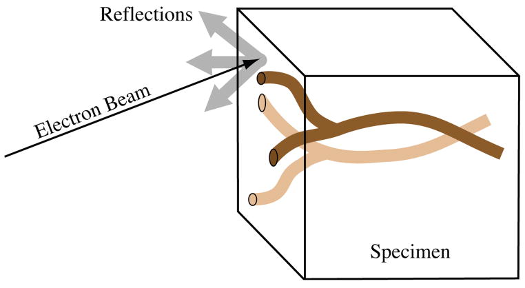
A new and promising technique for imaging large arrays of cells at nanometric resolution is serial block-face scanning electron microscopy (SBFSEM) [7], shown in Figure 1. In SBFSEM, each slice is cut away and discarded, and the electron beam is scanned over the remaining block face to produce electron backscattering images. An example image is shown in Figure 2. SBFSEM imaging has some advantages over other electron microscopic methods for the analysis of long axonal processes. Because the solid block is dimensionally stable, SBFSEM images have smaller deformations than serial-section transmission electron microscopy (TEM). The resolution and signal-to-noise properties of SBFSEM are generally not as good as TEM, but they are sufficient for manual tracing of individual axon paths. While three-dimensional (3D) data sets can also be obtained by electron microscope tomography (EMT) which has a resolution similar to TEM, it typically introduces reconstruction artifacts and does not provide the field of view (particularly in the z direction) needed to track neural processes across large distances.

Fig. 1.

Serial Block-Face Scanning Electron Microscopy

Fig. 2.

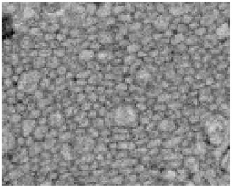
Sample Image from SBFSEM.

In this paper, we address the problem of automatically tracking individual axons in SBFSEM data sets. The particular application is the analysis of the optic tract in the embryonic zebrafish. Tracking individual axons is an essential step in analyzing the organization of the optic tract in wildtype and mutants. While, more generally, neurons are composed of dendrites, a cell body, synapses and an axon, here we focus on tracking axons, which are generally more difficult to track than dendrites because of their greater length and smaller diameter.

The challenges are that the axonal cross-sections (see Figure 2) are barely discernable by eye, and yet a large number of axons are tightly packed in the optic tract. The data acquired with SBFSEM does not have isotropic resolution: the out-of-plane resolution is significantly less (50 nm section thickness in the current data) than the lateral resolution of the slices. However, the block is oriented so that the imaged surface is nearly perpendicular to the axon axis to cut cross-sections through elongated processes. A single axon will traverse as many as 1000 cross-sectional slices, slowly winding its way in and around other axons. However, axons rarely branch or terminate, which aids in segmentation.

These SBFSEM datasets of the optic tract present, in some sense, a two-and-a-half dimensional data processing problem. Thus, we approach the problem of segmenting axons from electron microscopy images as a 2D segmentation problem combined with a tracking problem in the third dimension. This avoids the much more difficult full 3D problem of finding processes in noisy data amidst a dense packing of similar processes. This also allows an effective interface for user input. When the algorithm fails, the user can correct the segmentation and continue tracking. Completed axon pathways can also be viewed in two and three-dimensional plots.

There is some related work in the literature that applies computer vision and object tracking to medical data. For instance, Vazquez et al. introduced a semi-automatic, differential geometric method for segmenting neurons in 2D EM images [8]. In their method, a user initializes points on the boundary of the neuron, then a minimal length geodesic criterion is used to complete the boundary. Bertalmio et al. propose a slice-to-slice tracking/segmentation approach for electron microscopy images that uses 2D deformable curve models [9]. This method is similar to ours; however, tracking is not explicit, but is achieved indirectly with coupled partial differential equations. Furthermore, the tracked structures span a much smaller number of slices than axons. Researchers have also proposed segmentation methods for confocal microscopy images [10], [11]. Curvilinear structure detection has been studied in various applications, such as detection of blood vessels in magnetic resonance angiography data [12], [13]. These methods are tailored to the resolution and specific properties of their application domains and do not readily extend to tracking axons in electron microscopy images.

II. Methods

The field of computer vision provides numerous methods for tracking features through a set of images. By treating the 3D volume as a sequence of 2D images in time, feature tracking methods can be applied to the volume. We build our tracking application on the Kalman-snakes framework [14], [15]. The processing pipeline begins with a denoising of the input volume. Next, initial contours are computed at user defined axon locations in the first 2D slice. Each successive contour is tracked through the 3D volume using a Kalman filter combined with positional and velocity measurements.

A. Image Preprocessing

The SBFSEM data set used in our experiments has resolution 26 × 26 × 50 nm and has a relatively poor signal to noise ratio, partly due to non optimized specimen preparation. Given this resolution, and orienting the block such that the main axon bundles are roughly perpendicular to the imaging plane, axons range from 4 to 6 pixels in width in each 2D slice. Tracking such small features through a large number of slices is a challenging problem.

Denoising the data to obtain a cleaner representation of the axons is necessary as a preprocessing step. For this work, we used the UINTA algorithm [16] which denoises images by reducing the entropy of the density function associated with image neighborhoods. Figure 3 shows images before and after denoising. A 7 × 7 pixel neighborhood size was used, and 5 iterations of the filter were applied to each 2D slice of the SBFSEM volume. This denoising algorithm relies on nonparametric representation of the neighborhood statistics which it develops from samples from the image itself. Thus, UINTA learns the statistics of the image and reduces noise and enhances structure by reducing randomness. In this sense UINTA is particularly well suited for the highly repetitive (texture-like) structure of the block face images of the optic tract.

Fig. 3.

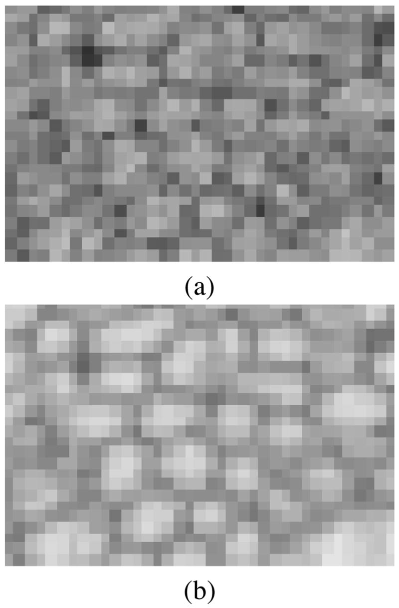
(a) a portion of a SBFSEM image, (b) after denoising.

B. Kalman Filter Based Axon Tracking

Axons have a tendency to “drift” and change shape through cross-sections, despite the near perpendicular arrangement of the cells to the cutting plane. For this reason, we implement a tracking algorithm that predicts the location of the axon in each slice. The framework in the Kalman filter allows us to follow an axon through several slices, with simple updates to position and velocity estimates.

1) Kalman Filter

Kalman filtering [17] provides a feedback control loop for predicting the location of the axon at each slice, sampling the image, and correcting the estimate. For each point on the axon contour, the filter updates the state,

$$w_k={[x_k,y_k,u_k,v_k]}^T$$ (1)

where [u_k, v_k] is the velocity at contour position [x_k, y_k]

Each iteration of the Kalman filter consists of three computations: a prediction, ŵ_k, measurement, z_k, and correction, w_k. A linear update using the previous state estimate, w_{k − 1}, gives the prediction state,

$${\widehat{w}}_k=A{w}_{k-1},$$ (2)

where

$$A=\left[\begin{array}{cccc}1& 0& 1& 0\\ 0& 1& 0& 1\\ 0& 0& 1& 0\\ 0& 0& 0& 1\end{array}\right].$$ (3)

The measurement state, z_k, is a combination of positions from active contour measurements (see Section II-B.2) and velocities from optic flow (see Section II-B.3). The filter combines the predicted and measured state to produce the corrected state estimate,

$$w_k={\widehat{w}}_k+K_k(z_k-H{\widehat{w}}_k),$$ (4)

where K_k is the Kalman gain matrix, given by

$$K_k={\widehat{P}}_k{H}^T{(H{\widehat{P}}_k{H}^T+R)}^{-1},$$ (5)

and P̂_k is the covariance of the current state estimate, given by

$${\widehat{P}}_k=A{P}_{k-1}{A}^{T}Q.$$ (6)

After each estimate, P_k is updated by

$$P_k=(I-K_{k}H){\widehat{P}}_k.$$ (7)

Q and R are constant diagonal matrices defining the process and measurement noise. H defines the relationship between the measurement and the model. For this model, H is the identity.

2) Positional Measurement — Active Contour Models

Active contour models [18], or snakes, are often used in image segmentation and feature tracking [14], [15]. Provided some user input or initialization, active contour models can lock onto and identify local features in an image. The Kalman filter uses the contour control points, [x_k, y_k], as part of its state model (described in Section II-B.1).

There are two main forces, E_int and E_image, that control the placement of the snake,

$$E_{\mathit{snake}}=\int \underset{E_{\mathit{int}}}{\underbrace{\alpha \mid v_s(s){\mid }^2+\beta \mid v_{ss}(s){\mid }^2}}+E_{\mathit{image}}(v(s))ds,$$ (8)

where v(s), v_s(s) and v_ss(s) are the parameterized contour model, its first derivative and second derivative with respect to arclength, respectively. The internal force, E_int, controls the smoothness of the contour while the external image force, E_image, acts as a weighted combination of edge and intensity information designed to fit the snake to axon membranes. Two free parameters in E_int, α and β, control how elastic and stiff the final snake will be with respect to the surrounding data points.

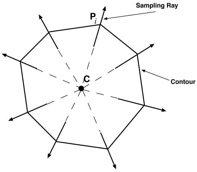
The set of contours used to define the axon in each slice is found using an iterative sampling process driven, in part, by the Kalman filter. The Kalman filter provides the algorithm with an initial set of predicted contour points. Assuming that each feature is roughly circular in shape and between 4 and 6 pixels in diameter, we sub-sample the image along a short ray, as shown in Figure 4. This sampling method prevents self-intersecting contours through the use of non overlapping rays. When the algorithm settles on a fit that minimizes the energy in E_snake, the Kalman filter is updated and a corrected contour is produced.

Fig. 4.

The contour is refined by iteratively sampling along the rays and recomputing the new edge location. We prevent self-intersecting contours by sampling along the ray from C, the midpoint of the contour, to P_i, a contour control point. New control points for each slice are repeatedly sampled computing new contours until they converge.

Axon tracking is initialized with a user defined point at the approximate center of the axon. The area immediately around this point is sampled for edges and the Kalman filter is initialized. The algorithm continues to track the axon in each slice, iteratively sampling the image data and updating the state estimate in the Kalman filter.

3) Velocity Measurement — Optic Flow

The shape and size of axonal cross-sections remain relatively constant as we move from one slice to the next, but their positions in the image change unless an axon runs exactly perpendicular to the imaging plane. The change in position is proportional to the angle between the axis of the axon and the imaging plane normal. We use this as our velocity component, [u_k, v_k], in the Kalman filter state estimate to help estimate the location of the axon in each slice.

The traditional method of estimating motion vectors from consecutive images is to use optic flow. Optic flow can be computed using eigenvectors of the piecewise-smooth structure tensor [19], [20]. In our data, the velocity field varies smoothly because nearby axons have similar orientations. Therefore, the structure tensor can be computed using Gaussian convolutions, which is computationally more efficient, instead of the nonlinear diffusion model. Let I and G_σ denote an input 3D intensity image and a 3D Gaussian kernel with standard deviation σ, respectively. We smooth the input image by convolution with G_σ: J = I * G_σ. Then the structure tensor is defined as

$$\mathcal{S}=G_{\rho }\ast (\nabla J\otimes \nabla J),$$ (9)

where G_ρ is another Gaussian kernel with standard deviation ρ and ⊗ is the vector outer product operation. Typically, σ is 1 pixel or less, whereas ρ is chosen to define the size of structures of interest [21]. For best results, we choose to fix σ = 0.6 and ρ = 5 pixels (approximate axon diameter). This tensor summarizes the first order neighborhood structure of axons: it has two large eigenvalues and one small eigenvalue. The eigenvector, e₁, associated with the smallest eigenvalue is oriented along the long axis of the axon. Since consecutive slices in a 3D volume represent fixed increments in the z position, Δz, the change in x − y position of points along the axon boundaries can easily be computed as

$$\mathrm{\Delta }x=\frac{e_{1,x}}{e_{1,z}}\mathrm{\Delta }z$$ (10)

$$\mathrm{\Delta }y=\frac{e_{1,y}}{e_{1,z}}\mathrm{\Delta }z$$ (11)

where e_1,x, e_1,y and e_1,z represent the x, y and z components of the eigenvector e₁ computed at the point of interest, respectively. Due to the alignment of the imaging plane perpendicular to the main running direction of the optic tract, individual axons are never parallel to the imaging plane; hence, the division by e_1,z does not pose a practical problem.

III. Results

Manual tracking of axons through a volume is tedious, requiring hours of careful labeling and correction. Automatic tracking allows for much faster annotation of axon locations. In this section, we present results with a 900 × 500 × 100 and a 900 × 500 × 700 volume. Image denoising with the UINTA algorithm and the computation of structure tensors take 20 minutes/slice and 10 minutes for the whole 100 slice volume, respectively, on a standard desktop PC. These steps are the computational bottlenecks; however, both can be performed offline. After these steps have been performed, tracking is initiated with a single mouse click inside the axon in the slice the user wants to start the tracking on. It takes approximately 2 seconds per slice to automatically track one axon through a volume. Users can scroll through slices in the volume, inspecting the tracking for errors and re-initializing the tracking if necessary.

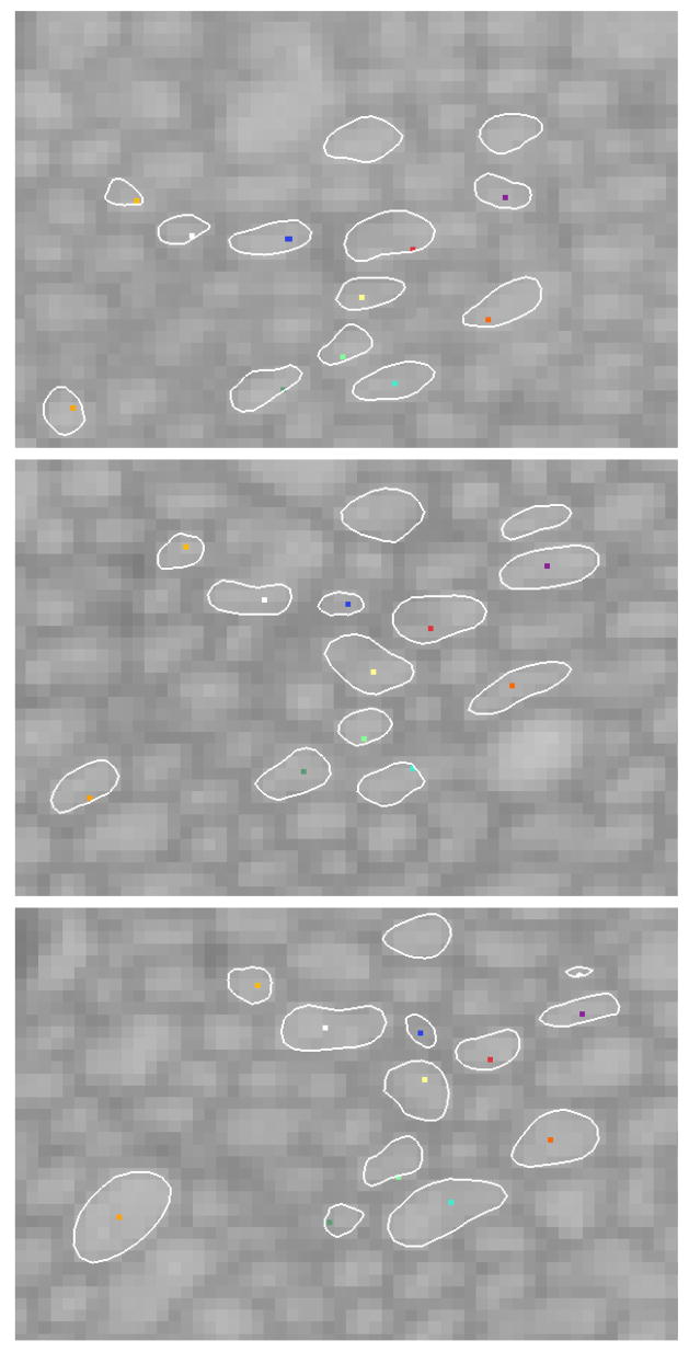
We validated our tracking algorithm against manual tracking by a human expert. The human expert tracked 17 axons, which were chosen for validation to represent a variety of difficulty levels for tracking. Easier-to-track axons maintain a clear boundary through the whole volume, whereas others may change shape rapidly. The manual tracking was performed by the expert clicking on an interior point of each axon in each slice. Figure 5 shows three different slices through a volume with the automatically detected axon contours (loops) and expert tracking (dots). To validate that the automatic tracking of an axon is correct in a given slice, we check whether (i) the human expert’s mark for that axon is found inside the automatic snake model, and (ii) the snake model has not grown to include other axons.

Fig. 5.

Sequence of axons tracked through 21 slices in a volume. Images are at slice 1, 11, and 21. Points inside the contour mark axons that have been tracked by an expert.

We performed two tracking tests. The first was 17 axons through 100 slices and the second, three axons through a much larger volume of 700 slices. In the 100 slice volume we were able to successfully track 16 of the 17 axons using our automated tracking approach. In the 700 slice volume, we tracked all three axons through 608 slices, and two through 657 slices. Hence, it is reasonable to expect that user intervention will only be necessary once every 100 slices per 20 axons. This translates into significant time savings over full-manual tracking. In addition, using the contour point locations from our tests, we generated 3D visualizations showing the structure of the axons, shown in Figure 6.

Fig. 6.

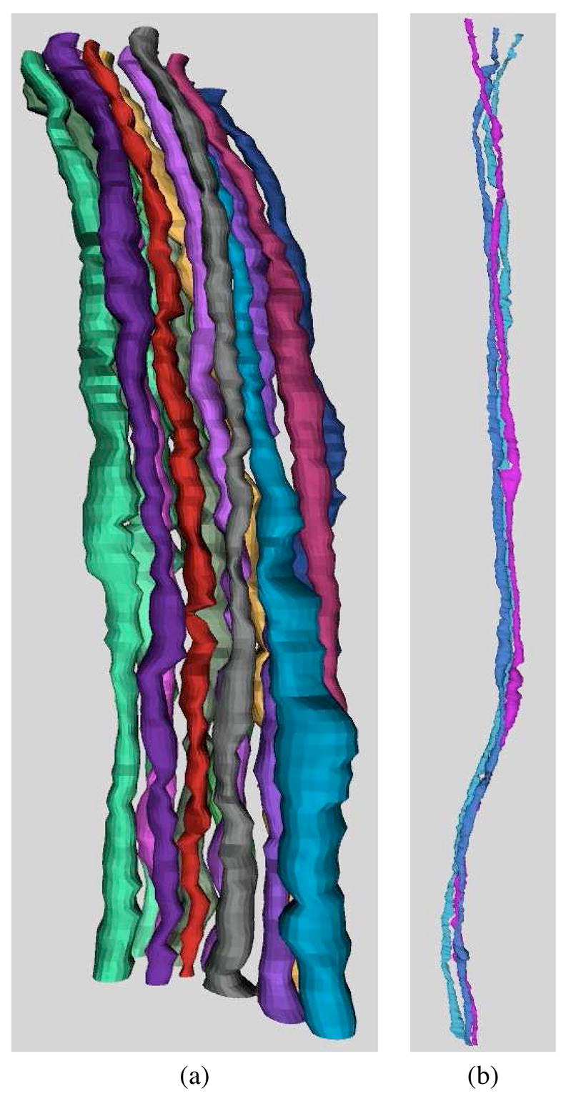
3D renderings using contour control points from each slice: (a) 16 axons tracked through 100 slices and (b) 3 axons tracked through 600 slices.

Figure 7 demonstrates the complex nature of the data. We tracked 4 axons using the automated method through a smaller and more difficult section of the volume. An expert guided the automated tracking, correcting the axon location when necessary.

Fig. 7.

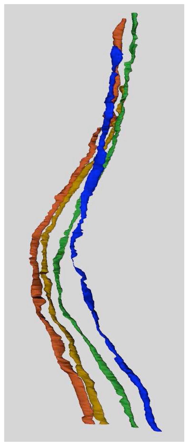
3D rendering of 4 axons through approximately 300 slices. This demonstrates the movement and twisting nature typical of features in these data. All tracking was verified by an expert.

Failure to track an axon results when an axon appears to split or become pinched. Figure 8 shows how the tracking fails when an edge appears in the middle of a feature separating the tracked axon from its actual path. It is also not unusual for a tracked axon to “latch” onto a neighboring axon and then find its way back to the correct axon within 3 or 4 slices. Parameters affecting the tracking include the α and β terms of the active contour and the measurement and noise covariance values in the Q and R matrices of the Kalman filter. Small changes to the Gaussian standard deviations in the structure tensor computation do not have an effect.

Fig. 8.

Common mode of failure over a sequence of slices. The tracked axon is shown in red with a loop and the expert tracked axon is the blue dot. The axon appears to split in the third image when the tracking picks up an edge (which first appears in the second image).

IV. Conclusions

The proposed system can successfully track axons through a series of slices in a volume. Denoising provides a clean view of the data in which to perform tracking. The Kalman filter predicts and corrects the placement of the axon in each slice using optic flow and active contours as velocity and position estimates. Initialization and correction of the algorithm is performed with user interaction. We presented a validation study that effectively tracked multiple axons through slices of a SBFSEM volume. Future work includes validating our tracking with more axons through larger volumes (of at least 1000 slices), using neighbor information to aid in more robust tracking, and performing the velocity estimation during tracking, rather than off-line.

The software to aid in the image processing was written using the Insight Segmentation and Registration Toolkit (ITK) [22]. The 3D axon renderings were created using the Visualization Toolkit (VTK) [23]. Currently, users can track by hand or with automatic tracking, including the ability to manually correct automatic tracking by reinitializing at desired locations.

References

- 1.Xiao YP, Wang Y, Felleman DJ. A spatially organized representation of colour in macaque cortical area v2. Nature. 2003;421(6922):535–539. doi: 10.1038/nature01372. [DOI] [PubMed] [Google Scholar]
- 2.Minsky. U.S. Patent number 301467 Microscopy apparatus.
- 3.Denk W, Strickler JH, Webb WW. Two-photon laser scanning microscopy. Science. 1990;248:73–76. doi: 10.1126/science.2321027. [DOI] [PubMed] [Google Scholar]
- 4.Fiala JC, Allwardt B, Harris KM. Dendritic spines do not split during hippocampal ltp or maturation. Nature Neuroscience. 2002;5(4):297–298. doi: 10.1038/nn830. [DOI] [PubMed] [Google Scholar]
- 5.Dacheux RF, Chimento MF, Amthor FR. Synaptic input to the on-off directionally selective ganglion cell in the rabbit retina. Journal of Comparative Neurology. 2003;456(3):267–278. doi: 10.1002/cne.10521. [DOI] [PubMed] [Google Scholar]
- 6.White JG, Southgate E, Thomson JN, Brenner FRS. The structure of the nervous system of the nematode caenorhabditis elegans. Phil Trans Roy Soc London Ser B Biol Sci. 1986;314:1–340. doi: 10.1098/rstb.1986.0056. [DOI] [PubMed] [Google Scholar]
- 7.Denk W, Horstmann H. Serial block-face scanning electron microscopy to reconstruct three-dimensional tissue nanostructure. PLoS Biol. 2004;2:11. doi: 10.1371/journal.pbio.0020329. [DOI] [PMC free article] [PubMed] [Google Scholar]
- 8.Vazquez L, Sapiro G, Randall G. Segmenting neurons in electronic microscopy via geometric tracing. Proc of ICIP. 1998:814–818. [Google Scholar]
- 9.Bertalmio M, Sapiro G, Randall G. Morphing active contours: A geometric approach to topology-independent image segmentation and tracking. Proc of ICIP. 1998:318–322. [Google Scholar]
- 10.Holmes DR, Moore MJ, Mantilla CB, Sieck GC, Robb RA. Rapid semi-automated segment. and analysis of neuronal morphology and func. from confocal image data. Proc of IEEE Int Sympo on Biomedical Imag. 2002:233–236. [Google Scholar]
- 11.Dima A, Scholz M, Obermayer K. Automatic segmentation and skeletonization of neurons from confocal microscopy images based on the 3-d wavelet transform. IEEE Trans on Image Processing. 2002;11(7):790–801. doi: 10.1109/TIP.2002.800888. [DOI] [PubMed] [Google Scholar]
- 12.Sato Y, Westin CF, Bhalerao A, Nakajima S, Shiraga N, Tamura S, Kikinis R. Tissue classificaion based on 3d local intensity structures for volume rendering. IEEE Trans on Visualization and Computer Graphics. 2000;6(2):160–180. [Google Scholar]
- 13.Lorigo LM, Faugeras O, Crimson WEL, Keriven R, Kikinis R, Nabavi A, Westin C-F. Codimension-two geodesic active contours for the segmentation of tubular structures. Proceedings of IEEE CVPR. 2000:444–451. [Google Scholar]
- 14.Terzopoulos D, Szeliski R. Active Vision. MIT Press; Cambridge, MA: 1992. Tracking with Kalman snakes; pp. 3–20. [Google Scholar]
- 15.Peterfreund N. Robust tracking of position and velocity with kalman snakes. IEEE Trans on Pattern Analysis and Machine Intelligence. 1999;21(6):564–569. [Google Scholar]
- 16.Awate Suyash P, Whitaker Ross T. Higher-order image statistics for unsupervised, information-theoretic, adaptive, image filtering. CVPR. 2005;(2):44–51. doi: 10.1109/TPAMI.2006.64. [DOI] [PubMed] [Google Scholar]
- 17.Andrew Blake, Rupert Curwen, Andrew Zisserman. A framework for spatio-temporal control in the tracking of visual contours. Real-time computer vision. 1995:3–33. [Google Scholar]
- 18.Kass M, Witkin A, Terzopoulos D. Snakes: Active contour models. International Journal of Computer Vision. 1988;1(4):321–331. [Google Scholar]
- 19.Liu H, Chellappa R, Rozenfeld A. Accurate dense optical flow estimation using adaptove structure tensors and a parametric model. Proc International Conference on Patter Recognition. 2002 doi: 10.1109/TIP.2003.815296. [DOI] [PubMed] [Google Scholar]
- 20.Brox T, Weickert J. DAGM. Springer-Verlag; 2002. Nonlinear matrix diffusion for optic flow estimation; pp. 446–453. [Google Scholar]
- 21.Scharr H, Weickert J. A scheme for coherence-enhancing diffusion filtering with optimized rotation invariance. Journal of Visual Communication and Image Representation. 2002 March/June;13(12):103–118. [Google Scholar]
- 22.http://www.itk.org, “NLM Insight Segmentation and Registration Toolkit,”.
- 23.http://www.vtk.org, “The visualization toolkit,”.